Predicting dust extinction from the stellar mass of a galaxy
Abstract
We investigate how the typical dust extinction of H luminosity from a star-forming galaxy depends upon star formation rate (SFR), metallicity and stellar mass independently, using a sample of 90,000 galaxies from Data Release 7 of the Sloan Digital Sky Survey (SDSS). We measure extinctions directly from the Balmer decrement of each source, and while higher values of extinction are associated with an increase in any of the three parameters, we demonstrate that the fundamental property that governs extinction is stellar mass. After this mass-dependent relationship is removed, there is very little systematic dependence of the residual extinctions with either SFR or metallicity, and no significant improvement is obtained from a more general parameterisation. In contrast to this, if either a SFR-dependent or metallicity-dependent extinction relationship is applied, the residual extinctions show significant trends that correlate with the other parameters. Using the SDSS data, we present a relationship to predict the median dust extinction of a sample of galaxies from its stellar mass, which has a scatter of mag. The relationship was calibrated for H emission, but can be more generally applied to radiation emitted at other wavelengths. These results have important applications for studies of high-redshift galaxies, where individual extinction measurements are hard to obtain but stellar mass estimates can be relatively easily estimated from long-wavelength data.
Keywords:
dust, extinction, galaxies: evolution, galaxies: high-redshift, galaxies: ISM1 Introduction
Galaxies which are currently forming stars emit a large fraction of their luminosity at ultraviolet (UV) wavelengths, where the output from young, massive stars peaks. Some fraction of this radiation is absorbed and re-emitted through the H recombination line, and the intrinsic luminosity of both of these indicators scales directly with the rate of formation of massive stars ( , with lifetimes less than Myr), giving a sensitive, well-calibrated probe of the current star formation rate (Kennicutt, 1998, SFR; e.g.). However, interstellar dust grains attenuate this short-wavelength radiation, reducing the observed flux and re-processing it into the far-infrared, so that only a small fraction of the intrinsic H or UV luminosity of a galaxy can be measured. Studies of star-forming galaxies are therefore hindered by uncertainties about the nature and amount of dust extinction which has occurred.
The typical H extinction of a galaxy, , can vary by several magnitudes and has been shown to depend upon galaxy properties such as luminosity (Wang & Heckman, 1996, e.g.), SFR (Hopkins et al., 2001; Sullivan et al., 2001; Berta et al., 2003; Garn et al., 2009b, e.g.), stellar mass (Brinchmann et al., 2004; Stasińska et al., 2004; Pannella et al., 2009, e.g.) and metallicity (Heckman et al., 1998; Boissier et al., 2004; Asari et al., 2007, e.g.). Explanations have been proposed for all of these effects: more massive galaxies may have built up a larger dust reservoir with which to attenuate H radiation; more actively star-forming galaxies are likely to have larger and more dusty star-forming regions; more metal-rich galaxies have a greater dust-to-gas ratio, and therefore higher extinction.
However, these studies have typically focused on one dependence at a time, and while they confirm that a single value of extinction should not be assumed for all galaxies, they do not address the question of whether stellar mass, SFR or metallicity is more fundamental. Further complications are introduced through the known correlations between galaxy properties – more massive galaxies tend to be more metal-rich (Tremonti et al., 2004; Kewley & Ellison, 2008, e.g.) and, amongst star-forming galaxies, more massive galaxies also have a greater typical SFR (Brinchmann et al., 2004, e.g.)11 1 The mass-SFR correlation breaks down for masses above those at which ‘SFR-downsizing’ has set in (Cowie et al., 1996, e.g.), whereby the most massive galaxies are no longer star-forming in the nearby Universe.. Recently Mannucci et al. (2010) have proposed the existence of a ‘fundamental metallicity relation’, whereby galaxies define a tight surface in the 3-dimensional space of mass, SFR and metallicity. They also argue that this surface does not evolve out to , and that previous observations that the trends between mass, metallicity and SFR evolve with redshift (Erb et al., 2006; Daddi et al., 2003; Maiolino et al., 2008, e.g.) arise because the high-redshift observations sample different regions of the surface. What is certainly clear is that the large number of competing effects make it difficult to determine what drives the observed systematic variation in dust extinction between different galaxies.
The most direct method of estimating extinction makes use of the strong wavelength-dependence of dust attenuation – by comparing the observed flux ratio of the H and H lines to the ratio that is expected in the absence of dust (the ‘Balmer decrement’), the amount of extinction at a given wavelength can be calculated. However, this method is only practical at low redshift, given the relative weakness of the H line, and the fact that the H line is redshifted out of the optical band at . If a suitable parameterisation for extinction could be calculated from galaxies in the local Universe, it could usefully be applied to the high-redshift population, where extinction cannot be estimated as easily.
In this work we aim to disentangle the effects that stellar mass, SFR and metallicity have upon dust extinction, determine which of these parameters is the most fundamental, and define a relationship to estimate the typical extinction of a galaxy when measurements of the Balmer decrement are not available. In Section 2 we present the data, describe our methods for selecting a clean sample of star-forming galaxies, and describe the estimates of SFR, stellar mass, metallicity and extinction that we use. Section 3 presents the observed variation in H extinction with each combination of galaxy parameters, and our models that describe how to predict dust extinction. In Section 4 we discuss these results, and their implications.
Throughout this work we assume a concordance cosmology of , and H km s-1 Mpc-1.
2 Data sample
2.1 Selection of a star-forming sample
In this work we make use of the superb spectroscopic information available from the Sloan Digital Sky Survey, Data Release 7 (Abazajian et al., 2009, SDSS DR7;). This dataset has been analysed by a group from the Max Planck Institute for Astrophysics, and Johns Hopkins University (hereafter the MPA/JHU group)22 2 http://www.mpa-garching.mpg.de/SDSS/DR7/ – descriptions of the analysis pipeline for a previous SDSS data release can be found in Brinchmann et al. (2004) and Tremonti et al. (2004). Spectroscopic redshifts and line fluxes (from a Gaussian fit to continuum-subtracted data, corrected for Galactic reddening) are provided for 927,552 sources at . We exclude from our analysis the sources spectroscopically classified as a ‘QSO’, sources outside the redshift range , within the redshift range (see Section 2.2.1), or sources with an uncertain estimate of their redshift (Z_WARNING ), and also remove multiple entries of a number of objects from the dataset (where we define a multiple entry to consist of two catalogued sources with angular separation less than 5 arcsec, and ). 617,822 sources are retained after these criteria have been applied.
In this work we require a sample of star-forming galaxies, from which we can measure an extinction and metallicity from emission-line ratios. In order to distinguish between star-forming galaxies and AGN, we use the ‘BPT’ (Baldwin, Phillips & Terlevich, 1981) emission line diagnostic, which compares the [O iii]5007/H and [N ii]6584/H line flux ratios. However, in order to use this diagnostic, all four emission lines must be detected with sufficient significance that accurate line flux ratios can be calculated. Note that the formal line flux uncertainties quoted in the MPA/JHU DR7 catalogue significantly underestimate the true errors – we have increased these uncertainties by the recommended factors of 2.473, 1.882, 1.566 and 2.039 for the H, H, [O iii] and [N ii] lines respectively, which were calculated by the MPA/JHU group through comparisons of the derived line fluxes of sources that were observed multiple times.

We perform a primary selection on the signal-to-noise (S/N) of the H line (we investigate possible biases of this selection method in Section 3.5), and measure the fraction of these sources that also have a detection of the other lines with a S/N of . Fig. 1 shows how the number of sources above a given H S/N ratio varies, along with the fraction of these sources with detections of the other emission lines above a given significance. It is clear that the limiting factor in this analysis is obtaining a secure detection of the [O iii] line – any sample with an H S/N threshold is essentially an [O iii]-selected sample.
For this analysis we set an H S/N requirement of 20, which includes 143,472 sources. We set an H S/N requirement of 3, which includes 99.97 per cent of these (i.e. we are not biasing the sample through our H cut). Of these sources, 99.86 per cent had a detection of the [N ii] line with S/N . In order to not bias our sample against weak [O iii] emitters (which have low metallicity; see Section 2.2), we reduce the [O iii] S/N threshold to 2. This cut includes 139,586 sources (97 per cent), in comparison to the 89 per cent which would have been selected above a S/N of 3. The Kauffmann et al. (2003b) criteria was then used to identify sources on the BPT diagram which are definitely star-forming (120,650 galaxies; 86 per cent of the sample).
2.2 Sample properties
2.2.1 Extinction
For each galaxy we measure the H to H line flux ratio, , and estimate an extinction at a particular wavelength , , using
| (1) |
where 2.86 is the intrinsic H/H line flux ratio that is appropriate for Case B recombination, a temperature of K and an electron density of cm-3 (Brocklehurst, 1971). We consider the accuracy of using the single value of 2.86 for all galaxies in Section 2.3.
We use the Calzetti et al. (2000) dust attenuation law to calculate the values of at the wavelengths of the H and H emission lines. This relationship was measured from observations of starburst galaxies, and has been shown to be appropriate for galaxies at redshifts up to (Garn et al., 2009b). Galaxies which had an observed value of were assigned an extinction of 0 mag (0.6 per cent of the sample).
An uncertainty in the extinction for each galaxy was calculated, using the H and H flux uncertainties and standard error propagation methods; the median uncertainty is 0.2 mag. The extinction errors were not found to correlate with any of the other properties of the sample, although a significant increase in the typical error was found for galaxies within the redshift range (median uncertainty of 0.34). This appears to be due to contamination of the redshifted H line with the [O i]5577 sky emission line (Osterbrock & Martel, 1992) – we reject from our analysis any sources within this redshift range.
2.2.2 Stellar mass
Stellar mass estimates, , have been calculated for the DR7 data by the MPA/JHU team33 3 http://www.mpa-garching.mpg.de/SDSS/DR7/Data/stellarmass.html, based upon fits to the total (CMODEL) SDSS photometry and following the philosophy of Kauffmann et al. (2003a) and Salim et al. (2007). We adopt these mass estimates, and we exclude from our analysis all galaxies (7 per cent of the remaining sample) where this estimate was not available. Note that the excluded galaxies have comparable properties to those retained, so this exclusion should not bias the results in any way.
Additional stellar mass estimates have been calculated from photometry measured within the 3 arcsec diameter SDSS fibres. A comparison of these two estimates allows us to define an effective aperture correction factor, which corresponds to the fraction of the stellar mass (and hence broadly, the stellar light) that is located within the fibre – this correction factor can be used to identify and reject highly extended galaxies, where the fibre-based spectroscopy will not be representative of the properties of the whole galaxy. This is effectively the same correction as is discussed by Hopkins et al. (2003), who use the ratio of total and fibre-based -band magnitudes to correct the detected H emission of SDSS galaxies.
Kewley et al. (2005) discuss the potential effects of estimating Balmer extinctions, metallicities and SFRs from spectroscopic observations made within a limited aperture, and conclude that an aperture covering factor of 20 per cent is sufficient to minimize systematic differences between these quantities and the global values. They recommend a minimum redshift of in order to obtain an average fibre-covering factor of greater than 20 per cent for a typical galaxy, which we have adopted for this analysis. We further reject galaxies at higher redshift that have a fibre-coverage factor per cent, along with a small number of galaxies where a conversion between point spread function magnitudes and fibre magnitudes performed by the MPA/JHU group has been unsuccessful (J. Brinchmann, private communication), leaving 95,240 galaxies in the sample (85 per cent of the galaxies which had stellar mass information available).
2.2.3 Star formation rate
In order to estimate SFRs, we calculate the intrinsic H luminosity for each galaxy, using the aperture and extinction-corrected H line flux. From this luminosity we calculate a SFR using the relationship in Kennicutt (1998), modified slightly to assume a Kroupa (2001) Initial Mass Function (IMF) that extends between 0.1 and 100 (to agree with the IMF used in the MPA/JHU stellar mass calculations). The choice of IMF is unimportant in this analysis as H emission is produced mainly by high-mass stars, where most IMFs agree. Implicit in our calculation of SFRs from an aperture-corrected H flux is the assumption that the radial distributions of H flux and stellar continuum are comparable – both Brinchmann et al. (2004) and Kewley et al. (2005) find that this is an acceptable approximation, if at least 20 per cent of the light of a galaxy is contained within the fibre.
2.2.4 Metallicity
We use the O3N2 indicator (Pettini & Pagel, 2004) as our proxy for ‘metallicity’ (denoting the gas-phase abundance of oxygen relative to hydrogen), where
| (2) |
We use this indicator for three reasons: (i) due to the similarity in wavelengths for the H and [N ii] lines, and the H and [O iii] lines, this indicator is essentially independent of the effects of dust attenuation; (ii) the O3N2 indicator has a unique metallicity for each line flux ratio (see Pettini & Pagel, 2004, for further details); (iii) the emission lines that are required to construct the O3N2 diagnostic are the same as we have used to select star-forming galaxies from the BPT diagram, and we can therefore measure a metallicity for our entire sample, without introducing additional selection criteria.
The conversion to an abundance comes from Pettini & Pagel (2004), , where they caution that the relationship may break down for low-metallicity galaxies with O3N2 , or – only 0.2 per cent of our sample have these values of O3N2, and we reject these from our analysis. All abundances can be converted to solar metallicities, using a value of (Asplund et al., 2004), and the range corresponds to .
2.2.5 Summary
| Reason | Ngals retained | % removed by cut |
|---|---|---|
| Initial Sample | 927,552 | – |
| Restrict to | 666,978 | 28.09% |
| Reject | 659,737 | 1.09% |
| Reject uncertain | 658,464 | 0.19% |
| Reject QSOs | 657,321 | 0.17% |
| Remove multiple entries | 617,822 | 6.01% |
| Require S/N (H)20 | 143,472 | 76.78% |
| Require S/N (H)3 | 143,433 | 0.03% |
| Require S/N ([NII])3 | 143,237 | 0.14% |
| Require S/N ([OIII])2 | 139,586 | 2.55% |
| Select as SF gals using BPT | 120,650 | 13.57% |
| Reject if no mass estimate | 112,008 | 7.16% |
| Reject if 20% fibre coverage | 95,240 | 14.97% |
| Restrict to O3N2 1.9 | 95,041 | 0.21% |
The details of the selection cuts applied to the sample are summarised in Table 1. The vast majority of the selection cuts are either bias-free (e.g. cuts in redshift), or remove so few galaxies that any bias must be insignificant. The possible exceptions to this are the selection of star-forming galaxies using a signal-to-noise threshold in H, the removal of galaxies without stellar mass estimates, and the fibre-coverage cut. As noted in Section 2.2.2, the properties (ie. magnitudes, redshifts, fluxes, emission line ratios, etc) of the galaxies excluded due to an absence of a mass estimate show a comparable distribution to those of the retained galaxies, so this cut is not expected to introduce any significant bias. The fibre coverage cut removes galaxies with larger angular sizes; these tend to be at the lower end of the redshift range, and to be amongst the more massive galaxies at those redshifts. This population of galaxies is well-represented at higher redshifts in the sample (where their angular sizes are smaller, but they remain luminous enough to be detected), so again their exclusion is expected to introduce only minimal bias. We conclude that the only selection cut which has the potential to introduce a significant bias is that of the H signal-to-noise threshold, and we will investigate this further in Section 3.5.
The final number of galaxies in our sample is 95,041, and Fig. 2 shows the distributions of , SFR, metallicity, redshift, extinction and extinction uncertainty. The median stellar mass is , with an inter-quartile range of to . The median SFR is 6.1 yr-1, with an inter-quartile range of 2.9 to 12.9 yr-1. The median metallicity is , or ; the metallicity distribution is asymmetric with an inter-quartile range of 8.61 to 8.78, and a longer tail towards low metallicities. The sample was restricted to a redshift range of and is mainly at (median = 0.085; inter-quartile range 0.067 to 0.113). The galaxies in the higher redshift tail predominantly have high masses and high SFR, but their extinction properties are comparable to those of lower redshift galaxies of the same mass and SFR – there is no evidence for redshift evolution within the sample. The median H dust extinction is 1.03 mag, close to the canonical value of 1 mag often assumed for H-selected galaxies. The median uncertainty in extinction estimates is 0.2 mag.

2.3 Accuracy of the extinction estimates
A previous SDSS data release has been analysed by the MPA/JHU group in the same manner as the DR7 data which we use in this paper. Brinchmann et al. (2004) have used these data to test the two assumptions that we have made, namely that the intrinsic H/H ratio is equal to 2.86, and that the conversion between intrinsic H luminosity and SFR that we use is appropriate for all galaxies. They conclude that both assumptions are suitable when used in combination with each other, although each is slightly incorrect – the Case B ratio depends upon temperature and density, varying between extremes of 2.72 (for K, cm-3) and 3.03 ( K, cm-3), while the most metal-rich galaxies produce a slightly lower H luminosity for the same SFR. Brinchmann et al. (2004) conclude that the combination of the two assumptions approximately cancel out when calculating the SFR, but there is the potential for a bias in our extinction estimates if the wrong intrinsic line ratio has been assumed. However, even the maximum error in our choice of Case B ratio would only lead to an error in extinction of mag, which is smaller than the typical uncertainty in the individual estimates of extinction.
In order to look for systematic offsets in our estimate of extinction with other properties of a galaxy, we match our SDSS sample with the 1.4-GHz Faint Images of the Radio Sky at Twenty-cm (Becker et al., 1995, FIRST;) survey, using the methodology described in Best et al. (2005). 2404 galaxies in our sample have a unique counterpart in FIRST, and for each galaxy we calculate a radio-based SFR using the relationship in Bell (2003), assuming that the radio spectrum of each galaxy can be modelled by (Garn et al., 2008, see e.g.). This SFR indicator has been shown to agree with infrared-based values for star-forming galaxies at redshifts up to (Garn et al., 2009a), and gives an independent estimate of the intrinsic SFR, without being biased by the effects of dust extinction.
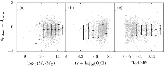
The resolution of FIRST is 5 arcsec, so the radio flux will be sampling a slightly larger, but comparable region of each galaxy to the SDSS fibres. We therefore compare the radio-based SFRs to SFRs calculated from the observed H flux, without correcting for extinction or aperture size, in order to obtain an estimate of the H dust extinction for each galaxy, , that is independent of the value calculated from the Balmer decrement, . Fig. 3(a) shows the agreement between these two extinction estimates – data have been binned by stellar mass, and for each bin we calculate the distribution of the value of . The median value of is taken to be our indicator of the ‘typical’ value, and the values of at the 16th and 84th percentiles () to indicate the range that each bin covers.
A systematic offset is seen for all bins, which is equivalent to having the radio SFRs systematically 30 per cent greater than the extinction-corrected H SFRs. This offset is likely to be due to the fact that the FIRST and SDSS observations are estimating their SFRs from different portions of a galaxy, although there may also be some contribution from a systematic uncertainty in the two SFR calibrations. However, no significant mass-dependent variation is seen between the two estimates of extinction. Fig. 3(b) and (c) show the equivalent plots for galaxies binned by metallicity and redshift – again, no significant variation is seen in the two extinction estimates. We do not show the equivalent plot for data binned by SFR, as this is affected significantly by sample bias due to the FIRST completeness limit of 0.75 mJy corresponding to a SFR limit that is significantly higher than that of the H selection.
The results of this section lead us to conclude that our extinction estimates are robust, and that our choice of a single value of the intrinsic H/H ratio should not introduce mass, metallicity or redshift-dependent trends into our analysis.
3 Results and analysis
3.1 Variation in H extinction with star formation rate, metallicity and stellar mass


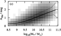
Fig. 4(a) shows the relationship between SFR and extinction for the galaxies in our sample – the grey-scale illustrates the region of extinction / SFR space that is populated with galaxies. In order to quantify the observed trend, we separate our sample into 20 logarithmically-spaced bins, selected by SFR. Within each bin, we calculate the distribution of measured H extinction values, which is overlaid (median, ). A clear increase is seen in the median extinction of galaxies with a higher SFR, in agreement with previous studies of the low-redshift Universe (Hopkins et al., 2001; Sullivan et al., 2001; Berta et al., 2003, e.g.).
Garn et al. (2009b) found that there was a well-defined relationship between dust extinction and SFR for a sample of H-emitting galaxies located at . Note that Garn et al. (2009b) calculated H extinction using an independent method (a comparison of H and 24-m SFR indicators, rather than from observations of the Balmer decrement). We overlay the Garn et al. (2009b) relationship on Fig. 4(a) – the relationship is in excellent agreement, with both the normalisation and the slope (despite hints of a slight change in the latter) consistent to within . This confirms the conclusions of that work, that the dependence of dust extinction on SFR does not change significantly between and (at least over the SFR range that was covered, 3 – 100 yr-1). This result also confirms that there should be no significant difference in the typical extinction relations for galaxies at different redshifts within our sample ().
We repeat this analysis to determine the variation in typical extinction with galaxy metallicity, which is shown in Fig. 4(b). As has been found in previous studies (Heckman et al., 1998; Boissier et al., 2004; Asari et al., 2007, e.g.), the typical extinction of a galaxy increases with metallicity and is approximately 1 mag for solar-metallicity galaxies, which have (Asplund et al., 2004).
Fig. 4(c) shows the equivalent results, binning the sample by stellar mass. The typical extinction of a galaxy increases with stellar mass, as has been found in previous studies (Brinchmann et al., 2004; Stasińska et al., 2004; Pannella et al., 2009, e.g.), and rises steadily between and . With the exception of the outer bins of data (which contain fewer galaxies) the typical 1 width of the distribution is mag, comparable to the distribution widths seen on the extinction / metallicity plot, and substantially smaller than the mag distribution width of the extinction / SFR plot.
3.2 Disentangling the relationships between H extinction and other galaxy properties
We have shown that the typical extinction of a galaxy correlates with its SFR, metallicity and stellar mass. In order to disentangle the complex relationships between these properties, we separate our sample by one of these properties into six sub-samples, and bin each sub-sample by both of the remaining two variables. For each bin, we calculate the distribution of H extinction (median ). The size of the SDSS DR7 dataset means that we can carry out this binning on a very fine scale – in the following analysis, any bins containing fewer than 20 galaxies are not shown for clarity, and contours illustrate the regions where bins contain more than 100 or 1000 galaxies.
We first take six sub-samples of galaxies with increasing metallicity, and calculate how extinction varies with mass and SFR for each of the sub-samples. If changes in metallicity are the dominant factor responsible for variations in the extinction of different galaxies, then we would expect to see an approximately constant extinction in each sub-sample, for any mass or SFR. However, Fig. 5 shows the results: while different metallicity galaxies populate different regions of the diagram, and the typical extinction of a galaxy does increase for the higher-metallicity sub-samples, there remains a significant variation in extinction within each plot (in the sense that extinction increases for higher masses or SFRs) that can not be explained purely through a metallicity dependence. The well-known correlation between stellar mass and SFR of star-forming galaxies can be seen in Fig. 5 through the direction of the contoured regions, and appears to be equally strong for galaxies of all metallicities.


Fig. 6 shows the equivalent results, for sub-samples of the data selected by SFR, and extinction as a function of mass and metallicity. The tight correlation between mass and metallicity means that the width of the region that is populated in each SFR sub-sample is relatively small. Tremonti et al. (2004) have identified that the correlation begins to break down at stellar masses above , with more massive galaxies not continuing to be more metal-rich – this effect can be seen clearly in Fig. 6. As for Fig. 5, a variation in the extinction of a galaxy within a given sub-sample can be seen, implying that variations in SFR are not the dominant factor responsible for differences in extinction between galaxies.
Fig. 7 shows the extinction as a function of SFR and metallicity, for sub-samples selected by their stellar mass. The same effect as before is apparent – different regions in the SFR / metallicity plane are populated by galaxies in each of the stellar mass sub-samples – and a weak anti-correlation between SFR and metallicity can be seen, for galaxies of a particular stellar mass. However, in contrast to the previous two figures, there is little variation in the median extinction of a galaxy at any populated point in each of the sub-samples. This implies that the majority of the variation in extinction between galaxies is driven by variations in stellar mass, rather than SFR or metallicity.
3.3 Principal component analysis
In order to quantify the relative importance of each of the parameters that we are considering, we normalise each to have zero mean and unit standard deviation, and calculate the covariance matrix of the resulting variables. Each entry in this matrix measures the strength of the linear dependence between two variables, and ranges between (a perfect correlation between the variables), 0 (no correlation) and (perfect anti-correlation). Table 2 reports the results: mass is strongly correlated with all the other variables, and SFR and metallicity are also strongly correlated with extinction.
| ‘SFR’ | ‘Mass’ | ‘Metallicity’ | ‘Extinction’ | |
|---|---|---|---|---|
| ‘SFR’ | 1.000 | 0.734 | 0.316 | 0.612 |
| ‘Mass’ | 0.734 | 1.000 | 0.717 | 0.719 |
| ‘Metallicity’ | 0.316 | 0.717 | 1.000 | 0.572 |
| ‘Extinction’ | 0.612 | 0.719 | 0.572 | 1.000 |
We use principal component analysis (Boroson & Green, 1992, PCA; e.g.) to quantify the relationships between these variables. This technique creates eigenvectors that are made up of linear combinations of the input variables, and are rotated to span the directions of maximum variance in the data. Principal component (PC) 1 contributes 71 per cent of the total variance, with weightings for the normalised SFR, mass, metallicity and extinction parameters as listed in Table 3 – i.e. the majority of the total variance in our sample can be explained simply by all four variables being correlated with each other, as has been found in previous sections. If all of the normalised quantities contributed equally to this PC, then they would all have weights of ; we find that mass contributes slightly more than metallicity or SFR to the first PC, but that all are broadly equivalent.
| ‘SFR’ | ‘Mass’ | ‘Metallicity’ | ‘Extinction’ | |
|---|---|---|---|---|
| PC1 (71%) | 0.469 | 0.559 | 0.453 | 0.512 |
| PC2 (17%) | 0.011 | 0.733 | ||
| PC3 (9%) | 0.313 | 0.331 | 0.237 | |
| PC4 (3%) | 0.760 |
PC2 contributes a further 17 per cent of the total variance, with significant weightings of for SFR and 0.733 for metallicity (see Table 3) – i.e. the majority of the remaining scatter in our data can be attributed to an anti-correlation between SFR and metallicity, for little variation in mass and extinction. A weak anti-correlation can be seen in each of the panels of Fig. 7 (as illustrated by the contoured regions). However, we have not fully removed the effects of stellar mass in these panels, as there is still a 0.5 dex variation in stellar mass across each of the sub-samples. Note that since the weightings of mass and extinction in PC2 are very small, the anti-correlation between SFR and metallicity will partially cancel out the correlation between SFR and metallicity from PC1.
The direction of PC2 implies that, if the stellar mass dependencies of other variables are removed from our dataset, we should see an anti-correlation between SFR and metallicity. In order to remove these dependencies, we bin the full dataset by stellar mass and fit a polynomial to the median mass and SFR for each bin, which gives
| (3) |
where .
We repeat this with the binned median mass and metallicity, to obtain
| (4) |
In both cases, moving to a higher-order polynomial did not significantly improve the fit.
We use these relations to predict the SFR and metallicity of all galaxies in the sample (the redshift range studied is sufficiently small that any cosmic evolution of these relations is negligible). By subtracting these predicted values from the observed values, we obtain the amount of SFR or metallicity variation that is not related to the overall stellar mass dependency, which we denote as the SFR and metallicity residuals. The relationship between SFR and metallicity residuals is shown in Fig. 8. An anti-correlation between SFR and metallicity, after stellar mass effects are removed, appears in the data for positive SFR residuals. Note that PCA only finds linear relationships between variables – as we have had to fit quadratics in order to represent the data successfully, we do not recover a pure anti-correlation between the two residuals.

Ellison et al. (2008) have found a similar trend that for a given stellar mass, galaxies with a high SFR have systematically lower metallicities than their low-SFR counterparts. They also find that more concentrated galaxies, with a smaller half-light radius, tend to be more metal-rich. Their interpretation of these results is that galaxies with a high surface mass density may have had a higher star formation efficiency in the past than their lower-density counterparts – this would lead to an increased production of metals, but lower current SFRs as more of the gas reservoir would have been depleted. This interpretation is consistent with our results.
PC3 contributes 9 per cent of the total variance, with the only significant weighting being for extinction. This may imply that there is a residual scatter in the extinction of each galaxy that is caused by some property other than mass, SFR or metallicity. PC4 contributes the remaining 3 per cent of the variance, and will be dominated by noise in the sample.
3.4 Modelling the variation in extinction
Having shown that extinction is correlated with various properties of a galaxy, we now attempt to model these variations, and identify the amount of information that is required in order to accurately estimate the typical extinction of a galaxy. We will quantify the accuracy of our models in two ways:
- 1.
calculating the residuals between the model and observed extinctions for all galaxies in our sample, and measuring the width of the Gaussian distribution that describes these residuals;
- 2.
plotting the distribution of residuals against galaxy mass, SFR and metallicity, in order to identify any significant trends that have not been accounted for in the models.
Our first model is the assumption that all galaxies can be represented by a single value of extinction, which we take to be the median value of in our sample, 1.03 mag. Fig. 9(a) shows that the distribution of residuals is roughly Gaussian, with width mag. The strong variations in extinction with SFR, metallicity or stellar mass are shown in Figs. 9(b) to (d), as previously identified in Section 3.1. We show both the uncertainty in the median estimate, and the distribution widths, in order to fully quantify the distribution. This model is the one most commonly used in the literature for H-selected samples, but is clearly not a good fit to the data.

Our next three models come from polynomial fits to the binned data from Section 3.1, in the form of
| (5) |
The extinction / SFR relationship, with , is well-fitted by a linear relationship. The extinction / metallicity relationship, with , requires a much higher-order polynomial (5th order) in order to model the curvature at high metallicities. We note here that it is unlikely that an extinction / metallicity relationship would be of much practical use – if sufficient spectroscopy exists that a reliable metallicity can be calculated, it would be better to measure extinction values directly. However, we include this model in our discussion for completeness. Finally, the extinction / stellar mass relationship, with , can be modelled by a 4th-order polynomial. These relationships are overlaid on Fig. 4 for reference, and all are a good fit to the binned data – we do not obtain a significantly better fit by moving to higher-order polynomials. The co-efficients of the polynomial fits are given in Table 4.
| Model | |||||
|---|---|---|---|---|---|
| SFR | 0.53 | 0.54 | |||
| Metallicity | 0.64 | 1.75 | 2.96 | -2.57 | -12.4 |
| Mass | 0.91 | 0.77 | 0.11 | -0.09 | |
| 1.11 | 0.69 | -0.19 | -0.18 |
The overall distributions of residuals are shown in Fig. 9(e), (i) and (m), and again are consistent with being Gaussian, with zero mean and widths of 0.33, 0.33 and 0.28 mag for SFR, metallicity and mass. All three models show significant improvement over the assumption of a single extinction for all galaxies. The contribution to these residuals from uncertainties in measuring the H and H fluxes is about 0.2 mag, from Fig. 2(f), which is about half of the total if errors are independent, and added in quadrature. Measurement errors in the SFR, metallicity and stellar mass parameters will account for some of the remaining scatter, but are unlikely to account for all. This suggests that there remains up to 0.2 mag of intrinsic scatter between different galaxies (cf. PC3 in Section 3.3).
The distribution of residuals for each of these models is shown in Fig. 9 as a function of SFR, metallicity and stellar mass, in order to test for remaining trends. By construction, the SFR residuals show no trend when the SFR model is used, and equivalent results are found for the other two models. However, the SFR model leads to a considerable variation in the residual extinction with either metallicity or stellar mass, in the sense that the model over-predicts the extinction of low-metallicity or low-mass galaxies. A similar result is found for the metallicity model, with extinction being over-predicted for low-SFR or low-mass galaxies. However, the mass model shows significantly smaller residual trends, as expected from the results of Section. 3.2 and Figure 7. This implies that it describes the data with less bias than the alternatives, although some weak trends with SFR and metallicity do still remain.
We attempt to improve upon the mass model, by adding a further SFR-dependent term to equation (5) with coefficients of and (the best-fit values after taking out the mass dependence); this will produce an improvement if the scatter around the SFR-mass relation correlates strongly with extinction. The results are shown in the bottom row of Fig. 9 – a slight improvement in the variation of residuals with SFR is seen (by construction), but the residuals show a worse trend with stellar mass than the previous model (since the strong SFR-mass correlation means that the additional SFR fit worsen the mass fit); the overall Gaussian width remains unchanged, at 0.28 mag. The largest residuals are seen at high stellar masses, possibly because this is the region where the mass / SFR correlation begins to break down, due to the effects of downsizing (where the most massive galaxies have already formed their stars, and undergo smaller amounts of current star formation than their less-massive counterparts). Concurrent fitting of the SFR and mass polynomials (even with the inclusion of cross-terms) was also attempted but does not decrease the overall Gaussian width of the residuals: although the trends of the residuals with SFR and mass improve slightly, those with metallicity worsen. Equivalent results are found if either a metal-dependent term is added to equation (5), or both a SFR-dependent and metal-dependent term are added, or all three terms are fitted concurrently – in all cases, the residuals are consistent with a Gaussian having a width of 0.28 mag. These results confirm that knowledge of stellar mass is sufficient to model the extinction of a galaxy in a statistical sense – once the mass variation is removed, very little improvement is obtained by a more complex model.
Finally, we note that very recently Mannucci et al. (2010) have proposed a ‘fundamental metallicity relation’, whereby galaxies define a tight surface in the 3-dimensional space of mass, SFR and metallicity. They introduce a new quantity, (Mass) - 0.32 (SFR), against which they argue that metallicity scatter of nearby galaxies is minimised. To test whether this can improve extinction estimates, we model the median extinction as a function of using a 4th-order polynomial (with co-efficients given in Table 4). However, we find that the resultant Gaussian width of the residuals relative to this model is 0.31 mag, with residual trends remaining with each of mass, SFR and metallicity that are worse than those of the mass model. We conclude that, for modelling extinction, the stellar mass alone provides a better (and simpler) input than .
3.5 H S/N bias
One of our primary selection requirements was that sources have an H S/N ratio greater than 20, as measured from the observed line flux. By doing this, we are implicitly biasing our sample against highly extinguished sources – the error on the line flux measurement will be independent of the extinction of a galaxy, while the observed flux will be lower for galaxies with higher extinction.
In order to confirm that this bias does not significantly influence our conclusions, we repeat our analysis using an alternative selection procedure which is less prone to an extinction bias. For galaxies in which the H and H emission lines are both detected with S/N ratio greater than 3, we use equation (1) to calculate the H extinction. Similarly, for those galaxies with H S/N ratio above 3, but H S/N ratio below 3, we estimate the extinction using the 3 limit on the H flux (strictly this is a lower limit on the extinction). We then correct the H line fluxes for the calculated extinction, and derive the S/N ratio with which the H line would have been detected in the absence of extinction. We then set a primary selection requirement that this unextinguished H S/N ratio should be greater than 75, and we repeat the analysis of the paper. This selection procedure does not completely remove the effects of extinction bias (the most extinguished sources may still be excluded if their observed H S/N ratio is below 3, or if their H line is undetected leading to an underestimated extinction and undercorrection of their H flux), but it does greatly reduce the bias. Therefore, if the same trends are found, that would provide confidence in their reliability.
The median extinction of H in the new sample is 1.35 magnitudes, significantly higher than the previous selection. This increase is driven both by the exclusion of low-extinction galaxies (mostly at lower masses; these were in the original sample but fail to reach the higher threshold for the revised sample) and by the inclusion of additional high-extinction galaxies (especially at higher masses). We re-calculate the relations with extinction determined in Section 3.4. The fitted polynomial parameters for the mass / extinction relationship are , , and ; this has almost exactly the same shape as the previous relation, but is shifted up by about 0.18 magnitudes of extinction. Equivalent shifts are seen in the extinction relationships with other parameters. The distributions of extinction residuals (cf. Fig. 9) again show similar trends, with a scatter of 0.40 around the median extinction value being reduced to 0.37, 0.34 and 0.28 when taking out the SFR, metallicty and mass models, respectively. This confirms that mass is the predominant factor influencing the extinction of galaxies; once again, adding in additional SFR- or metallicity-dependent terms does not further decrease the scatter.
These tests leads us to conclude that although we are excluding some of the more highly extinguished sources from our sample, the trends determined from the analysis are robust.
4 Discussion and Conclusions
We have used the superb spectroscopic coverage of SDSS DR7 to disentangle the effects of three of the physical parameters that are known to correlate with the dust extinction of a galaxy. We select a clean sample of star-forming galaxies using the BPT diagram, and calculate extinctions from observed Balmer decrements. We calculate metallicities from the O3N2 indicator, and after correcting for dust extinction and aperture size, we calculate SFRs from the H line. Stellar mass estimates have been calculated independently by the MPA/JHU group.
We confirm that the typical dust extinction of a galaxy increases with greater SFR, metallicity or stellar mass. By selecting various sub-samples of galaxies, we show that the dominant factor is stellar mass – we conclude that the observed correlations between extinction and SFR, or extinction and metallicity, are largely secondary effects brought about by the known dependence of these parameters on the stellar mass of a galaxy. The implications that we draw from our results are:
- •
As galaxies build up their stellar mass over time, they also build up their dust content. This increase in dust leads to a greater H extinction, and therefore a dependence of extinction on stellar mass is seen.
- •
Massive galaxies are able to retain a greater fraction of the metals that they produce, due to their deep potential wells, while less-massive galaxies lose metals from their shallower potential wells through the effects of galactic winds (Tremonti et al., 2004, e.g.). A relationship between metallicity and extinction is therefore formed – this is a secondary effect brought about by the dependence of both extinction and metallicity on stellar mass.
- •
More massive galaxies are capable of forming a greater amount of stars in a starburst, and therefore a relationship between the SFR and extinction of a galaxy is set up – this is also a secondary effect brought about by the relationship between SFR and stellar mass. This relationship will only hold for galaxies that are currently forming stars, and will break down at the highest masses, since these galaxies formed their stars at earlier epochs (Cowie et al., 1996). However, extremely high-mass galaxies are poorly represented in our sample, since it was selected by the presence of H emission to be undergoing current star formation.
- •
An anti-correlation is seen between SFR and metallicity, for galaxies of a given stellar mass. This may be due to variations in star formation efficiency between galaxies, as discussed by Ellison et al. (2008), where galaxies that have formed more stars in the past have a lower current SFR, and higher metallicity.
Using equation (5) it is possible to predict the extinction of a galaxy with a given stellar mass, to within a typical error of 0.28 mag (note that as discussed in Section 3.5, samples selected with different selection effects may require small offsets in normalisation of this equation, but the functional form and the scatter around it is largely robust to changes in selection technique). This typical error is broadly comparable to the accuracy with which extinctions can be estimated from the Balmer decrement, for our sample of galaxies selected with an H S/N ratio , although this comparison will of course depend upon the S/N ratio of available H and H observations. We believe that the stellar mass of a galaxy is the best indicator to use when estimating the typical amount of dust extinction, both because it appears to be the fundamental parameter that governs dust extinction, and also because it can be estimated in a way that is almost unaffected by dust, using the rest-frame -band luminosity alone (Longhetti & Saracco, 2009, e.g.). For some applications, it might be simpler to use the SFR-dependent correction (for example, correcting an observed H or UV luminosity function for the effects of dust). However, we caution that this form of correction has the potential for introducing a significant mass-dependent bias into the results, and should be used with care.
Estimating the extinction of truly ‘passive’ galaxies (with SFR yr-1) is outside the scope of this work, as these are not detected in our H selected samples. However, for massive galaxies, we note that the H selection limit corresponds to star formation rates well over an order of magnitude below their historical average. These galaxies display high levels of extinction, implying that high-mass ‘passive’ galaxies are also likely to have high levels of extinction of the small amount of H emission that they do produce.
We note that although all of our results have been derived for H extinction, they can be generally applied to line emission at another wavelength through the use of equation (1) and the Calzetti et al. (2000) dust attenuation law. If the extinction of UV radiation is required, rather than line emission, then a factor of 0.5 needs to be applied to this equation – see Calzetti et al. (2000) and Garn et al. (2009b) for further details.
Estimates of star-formation at high redshift () are commonly made using a wide range of different estimators: UV continuum; [OII] or H emission lines; sub-mm, mid-IR or far-IR continuum; radio emission. Each of these has their own advantages and disadvantages, with different sensitivities, angular resolutions, reliability of calibration, and effects of dust extinction (Kennicutt, 1998, cf.). The latter effect is particularly important for star-formation rates estimated from H or UV selected samples (the most sensitive selection methods currently available); previous star-formation rate estimates from such samples have either required assumptions about the global extinction of all galaxies (e.g. a constant – a hypothesis which can be ruled out by the results in this work), spectroscopic observations of each galaxy to measure individual dust extinctions (time-consuming, and technically challenging at high redshift), or a sufficiently large number of photometric data-points to enable SED-fitting techniques to estimate extinctions without issues of degenerate solutions. The results presented in this work suggest that a representative extinction correction can be derived from the mass, which can be estimated using far fewer photometric data points. Provided that the relation between mass and extinction is confirmed to be independent of redshift, this result could have important applications for studying large samples of star-forming galaxies, especially at high redshifts.
Acknowledgements
This paper is dedicated to the memory of, and in tribute to, Timothy Garn. Timothy had largely completed the analysis and writing of the paper before his untimely death, and PNB put the finishing touches to it. PNB is grateful for support from the Leverhulme Trust. The authors thank Jarle Brinchmann for providing advice on using the MPA/JHU catalogues, and making the duplicate source list available. PNB thanks the anonymous referee for helpful comments.
References
- Abazajian et al. (2009) Abazajian K. N., et al., 2009, ApJS, 182, 543
- Asari et al. (2007) Asari N. V., Cid Fernandes R., Stasińska G., Torres-Papaqui J. P., Mateus A., Sodré L., Schoenell W., Gomes J. M., 2007, MNRAS, 381, 263
- Asplund et al. (2004) Asplund M., Grevesse N., Sauval A. J., Allende Prieto C., Kiselman D., 2004, A&A, 417, 751
- Baldwin et al. (1981) Baldwin J. A., Phillips M. M., Terlevich R., 1981, PASP, 93, 5
- Becker et al. (1995) Becker R. H., White R. L., Helfand D. J., 1995, ApJ, 450, 559
- Bell (2003) Bell E. F., 2003, ApJ, 586, 794
- Berta et al. (2003) Berta S., Fritz J., Franceschini A., Bressan A., Pernechele C., 2003, A&A, 403, 119
- Best et al. (2005) Best P. N., Kauffmann G., Heckman T. M., Ivezić Ž., 2005, MNRAS, 362, 9
- Boissier et al. (2004) Boissier S., Boselli A., Buat V., Donas J., Milliard B., 2004, A&A, 424, 465
- Boroson & Green (1992) Boroson T. A., Green R. F., 1992, ApJS, 80, 109
- Brinchmann et al. (2004) Brinchmann J., Charlot S., White S. D. M., Tremonti C., Kauffmann G., Heckman T., Brinkmann J., 2004, MNRAS, 351, 1151
- Brocklehurst (1971) Brocklehurst M., 1971, MNRAS, 153, 471
- Calzetti et al. (2000) Calzetti D., Armus L., Bohlin R. C., Kinney A. L., Koornneef J., Storchi-Bergmann T., 2000, ApJ, 533, 682
- Cowie et al. (1996) Cowie L. L., Songaila A., Hu E. M., Cohen J. G., 1996, AJ, 112, 839
- Daddi et al. (2003) Daddi E., et al., 2007, ApJ, 670, 156
- Ellison et al. (2008) Ellison S. L., Patton D. R., Simard L., McConnachie A. W., 2008, ApJ, 672, L107
- Erb et al. (2006) Erb D. K., Shapley A. E., Pettini M., Steidel C. C., Reddy N. A., Adelberger K. L., 2006, ApJ, 644, 813
- Garn et al. (2008) Garn T., Green D. A., Riley J. M., Alexander P., 2008, MNRAS, 387, 1037
- Garn et al. (2009a) Garn T., Green D. A., Riley J. M., Alexander P., 2009a, MNRAS, 397, 1101
- Garn et al. (2009b) Garn T., Sobral D., Best P. N., Geach J. E., Smail I., Cirasuolo M., Dalton G. B., Dunlop J. S., McLure R. J., Farrah D., 2009b, MNRAS, in press (astro-ph/0911.2511)
- Heckman et al. (1998) Heckman T. M., Robert C., Leitherer C., Garnett D. R., van der Rydt F., 1998, ApJ, 503, 646
- Hopkins et al. (2001) Hopkins A. M., Connolly A. J., Haarsma D. B., Cram L. E., 2001, AJ, 122, 288
- Hopkins et al. (2003) Hopkins A. M., et al., 2003, ApJ, 599, 971
- Kauffmann et al. (2003a) Kauffmann G., et al., 2003a, MNRAS, 341, 33
- Kauffmann et al. (2003b) Kauffmann G., et al., 2003b, MNRAS, 346, 1055
- Kennicutt (1998) Kennicutt R. C., 1998, ARA&A, 36, 189
- Kewley & Ellison (2008) Kewley L. J., Ellison S. L., 2008, ApJ, 681, 1183
- Kewley et al. (2005) Kewley L. J., Jansen R. A., Geller M. J., 2005, PASP, 117, 227
- Kroupa (2001) Kroupa P., 2001, MNRAS, 322, 231
- Longhetti & Saracco (2009) Longhetti M., Saracco P., 2009, MNRAS, 394, 774
- Maiolino et al. (2008) Maiolino R., et al., 2008, A&A, 488, 463
- Mannucci et al. (2010) Mannucci F., Cresci G., Maiolino R., Marconi A., Gnerucci A., 2010, MNRAS, submitted, arXiv:1005.0006
- Osterbrock & Martel (1992) Osterbrock D. E., Martel A., 1992, PASP, 104, 76
- Pannella et al. (2009) Pannella M., et al., 2009, ApJ, 698, L116
- Pettini & Pagel (2004) Pettini M., Pagel B. E. J., 2004, MNRAS, 348, L59
- Salim et al. (2007) Salim S., et al., 2007, ApJS, 173, 267
- Stasińska et al. (2004) Stasińska G., Mateus A., Sodré L., Szczerba R., 2004, A&A, 420, 475
- Sullivan et al. (2001) Sullivan M., Mobasher B., Chan B., Cram L., Ellis R., Treyer M., Hopkins A., 2001, ApJ, 558, 72
- Tremonti et al. (2004) Tremonti C. A., et al., 2004, ApJ, 613, 898
- Wang & Heckman (1996) Wang B., Heckman T. M., 1996, ApJ, 457, 645