Mass measurements in the vicinity of the doubly-magic waiting point ⁵⁶Ni

The cyclotron resonance frequencies were fitted with the theoretical lineshape [22, 24, 25] (see Fig. 1). The measured frequencies were corrected for the count-rate-effect [27] whenever it was possible. For the lower statistics files, where the count-rate-class analysis was not possible, the statistical error was multiplied by a factor obtained from a comparison of the errors in the frequencies of all higher-statistics files with and without the count-rate-class analysis. The magnetic field $B$ at the time of measurement was interpolated from the well-known reference measurements before and after the measurement. The frequency ratio $r$ of the well-known reference ion to the ion of interest was determined (see Eq. 1). This ratio gives the mass ratio of the ion of interest to the reference ion (see Eq. 2),

In order to take into account fluctuations in the magnetic field, a correction of $\delta_{B}(\nu_{ref})/\nu_{ref}=5.7(8)\times 10^{-11}\text{min}^{-1}\Delta t$, where $\Delta t$ is the time between the two reference measurements, was quadratically added to the statistical uncertainty of each frequency ratio. The weighted mean of the measured frequency ratios was calculated and used as the final value. The inner and outer errors [28] of the data sets were compared and the larger value of these two was taken as the error of the mean. Finally, the uncertainty due to mass-dependent shift $\delta_{m,lim}(r)/r=(7.5\pm 0.4\times 10^{-10}/u)\times\Delta m$ [13] and an additional residual relative uncertainty $\delta_{res,lim}(r)/r=7.9\times 10^{-9}$ [13] were quadratically added to the error.

In order to evaluate the masses of the measured nuclides, a least-squares adjustment was done in a similar manner as in Refs. [30, 29, 31]. Here, we follow the notations used in those references. The input data $q_{i}$ for the least-squares method consist of the measured 17 frequency ratios between 13 nuclides (see Table 2) and the current mass values for the 13 nuclides from the Atomic Mass Evaluation 2003 (AME03) [29]. Thus, we have 30 input data to 13 nuclides involved in the frequency ratio measurements forming an overdetermined system.

The input data of the thirteen AME03 values are simply $q_{i}=m_{i}\pm\delta m_{i}$. For the frequency ratios, a similar procedure as in Ref. [31] was applied. Eq. 2 can be expressed as a linear equation in $m$:

In order to have the left side independent of the ratio $r$, a constant factor $C=A/A_{ref}$, where $A$ and $A_{ref}$ are the mass numbers of the reference ion and the ion of interest, is introduced. Then, a term $-C\cdot m_{ref}$ is added on both sides of Eq. 3:

Including the uncertainties $\delta r$, $\delta m_{ref}$, and $\delta m_{e}$, Eq. 4 yields:

In Eq. 5, the terms $\delta m_{e}(1-r)$ and $m_{e}\delta r$ have been neglected since they are small compared to $m_{ref}\delta r$. Since the left-side of Eq. 5 is a continuous and differentiable function of $m$, a least-squares fit to this linear, overdetermined system can be applied following Ref. [30]. The measured data $q_{i}$ are obtained from Eq. 6 with the uncertainties $dq_{i}$ given in Eq. 7:

Let the vector $\left|m\right\rangle$ represent the masses of 13 nuclides involved in the frequency ratio measurements and the vector $\left|q\right\rangle$ corresponds to the input data (17 rows obtained from Eq. 6 and 13 rows representing the AME03 mass values of the nuclides). Then, a $30\times 13$ matrix $K$ representing the coefficients $K\left|m\right\rangle=\left|q\right\rangle$ and a $30\times 30$ diagonal weight matrix $W$ with the elements $w_{i}^{i}=1/dq_{i}^{2}$ can be formed. The solution of the least-squares method yields a vector of adjusted masses $\left|\overline{m}\right\rangle=A^{-1}$${}^{t}KW\left|q\right\rangle=R\left|q\right\rangle$ where $A^{-1}$ is the inverse of the normal matrix $A=~^{t}KWK$ which is a positive-definite and invertible square matrix of the order of $13$. The errors for the adjusted masses $\overline{m_{i}}$ are obtained as a square-root of the diagonal elements of the matrix $A^{-1}$.

The adjusted data $\left|\overline{q}\right\rangle$ can be calculated as $\left|\overline{q}\right\rangle=KR\left|q\right\rangle$. Now, if the uncertainties $dq_{i}$ are very small for this overdetermined system (the number of input data $N_{d}=30$ $>$ the number of variables (masses) $N_{v}=13$), the normalized deviation between the adjusted data $\overline{q_{i}}$ and input data $q_{i}$ should have a Gaussian distribution with $\sigma=1$. For $N_{d}-N_{v}=30-13=17$ degrees of freedom, this gives a $\chi^{2}$ equal to

The consistency can also be expressed as normalized $\chi$:

for which the expected value is $1\pm 1/\sqrt{2(N_{d}-N_{v})}$.

The influence of each datum $i$ on a mass $m_{\nu}$ can be seen from the $(i,\nu)$ element of a flow-of-information matrix $F=~^{t}R\otimes K$ ($30\times 13$ matrix) [30]. Each column of $F$ represents all the contributions from all input data to a given mass $m_{\nu}$. The sum of these contributions is 1. The sum of influences along each row shows the significance of that datum.

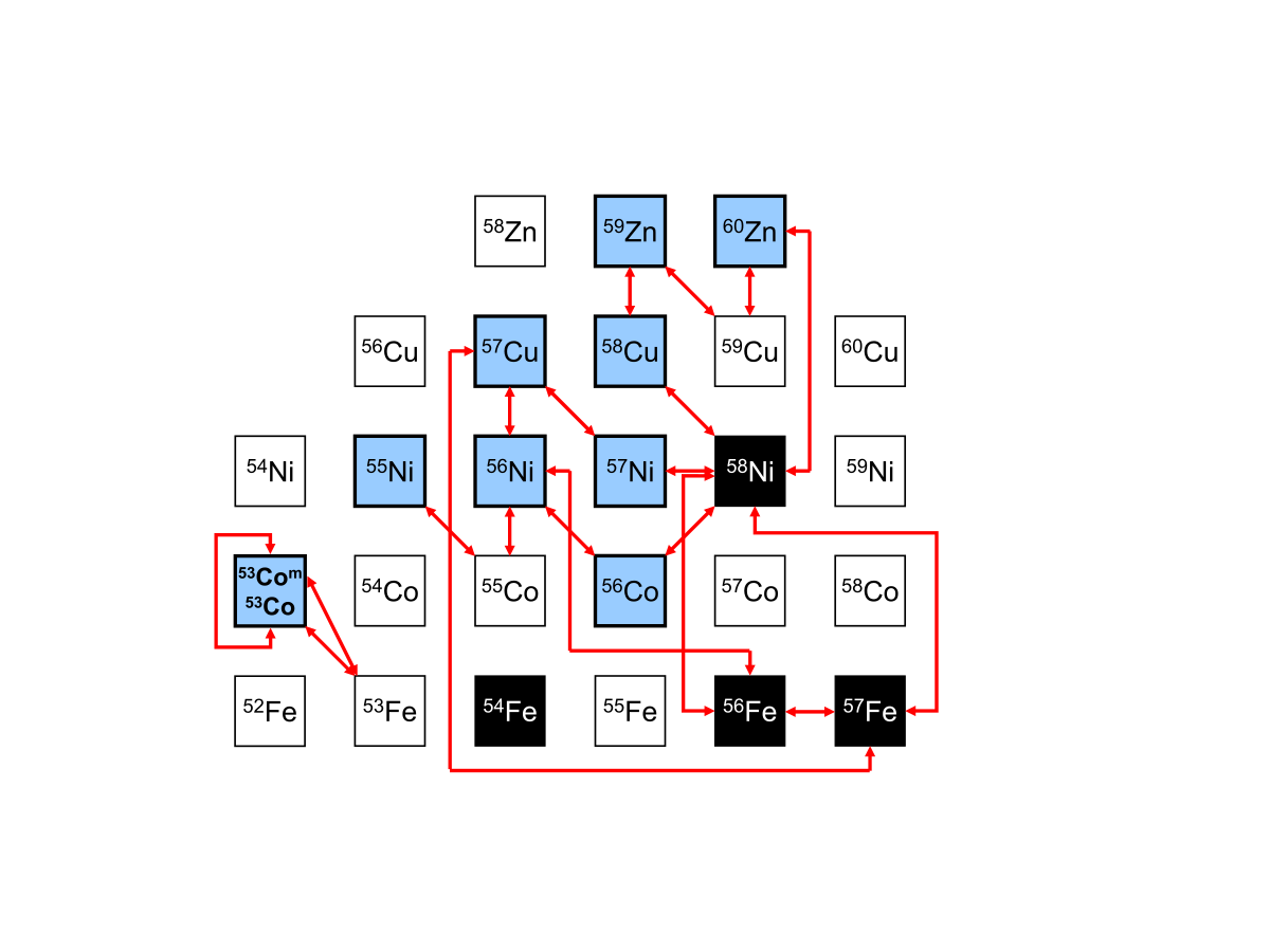
Altogether 20 frequency ratios were measured in this work (see Table 2). The number of measured frequency ratios is high because the reference nuclides in this mass region are known with quite a modest precision of about $0.6-2~\text{keV}$ or $\delta m/m\approx 1.1-4.1\times 10^{-8}$. Therefore, a small network of measurements provides more accurate mass values for the measured nuclides. In addition, some $Q_{\text{EC}}$ and $S_{p}$ values were measured directly to obtain a better precision.

The nuclides other than ⁵³Co and ⁵³Co^m, formed a network of $13$ nuclides and $17$ measured frequency ratios. For these nuclides, a least-squares method described in Sec. III.2 was applied and adjusted mass values were obtained. The normalized $\chi=1.08$ was well within the expected value $1.00\pm 0.17$, and therefore, no additional error was added to the frequency ratios. The biggest contribution to the $\chi^{2}$ value ($27~\%$) comes from the ⁵⁸Cu AME03 mass value which is $3.6(17)~\text{keV}$ higher than the adjusted value obtained with the JYFLTRAP results. In addition to ⁵⁸Cu, also the AME03 values of ⁵⁵Co (13 %), ⁶⁰Zn (10 %), ⁵⁹Zn (8 %)and ⁵⁸Ni (7 %) have a substantial contribution to the $\chi^{2}$ value. This is also seen in the adjusted values which deviate from the AME03 values of these nuclides.

In the following, the mass excess results for the radioactive nuclides are compared to earlier experiments (see Figs. 4, 5, 6, and 7) and discussed nuclide by nuclide. The results for the nuclides mainly used as references are also summarized (see Figs. 8, 9, and 10). The directly measured values were used for ⁵³Co and ⁵³Co^m. For the rest, the adjusted mass values (see Table 3) were applied. The results of ⁵³Co and ⁵³Co^m include also a new value for the excitation energy of the high-spin isomer.

The $Q_{\text{EC}}$ values are directly obtained by measuring the frequency ratio $r$ between the beta-decay mother (mass $m_{m}$) and daughter (mass $m_{d}$) in a Penning trap:

With this method, the $Q_{\text{EC}}$ values can be determined to high precision even if the reference (daughter) nuclide has a moderate precision. The mass excesses for the daughter nuclides were taken from the adjusted mass values (Table 3).

The $Q_{\text{EC}}$ values are tabulated in Table 4. The mirror-decay $Q_{\text{EC}}$ values of $T=1/2$ nuclides ⁵³Co, ⁵⁵Ni, ⁵⁷Cu, and ⁵⁹Zn as well as the $Q_{\text{EC}}$ values for the $T_{Z}=0$ nuclides ⁵⁶Ni and ⁵⁸Cu in the $T=1$ triplets at $A=56$ and $A=58$ were directly determined from the frequency ratio measurements against their beta-decay daughters. In addition, the $Q_{\text{EC}}$ value for the spin-gap isomer ⁵³Co^m was measured relative to the ⁵³Fe ground state. ⁵³Co^m decays dominantly to its isobaric analogue state (IAS) at $3040.4(3)~\text{keV}$ in ⁵³Fe [78] for which a $Q_{\text{EC}}$ value of $8421.8(12)~\text{keV}$ is obtained. The $Q_{\text{EC}}$ value for ⁶⁰Zn was determined from the adjusted mass value for ⁶⁰Zn and the AME03 value for ⁶⁰Cu [29].

Recently, corrected $ft$ values, $\mathcal{F}t$, have been calculated for $T=1/2$ mirror transitions up to ⁴⁵V [8, 9]. The $Q_{\text{EC}}$ values measured in this work offer a possibility to expand these studies from ⁵³Co up to ⁵⁹Zn. Table 5 summarizes the current averages of half-lives and branching ratios as well as electron-capture probabilities needed to calculate the $ft$ value. Experimental Gamow-Teller matrix elements $\left|\left\langle\sigma\tau\right\rangle\right|$ have been calculated from the Gamow-Teller strength $B(GT)$:

where the constant $C=2\cdot\overline{\mathcal{F}t}^{0^{+}\rightarrow 0^{+}}=6143.5(17)~\text{s}$ [80], $B(F)$ is the Fermi strength, which equals $1$ for $T=1/2$ mirror decays, and $g_{A}/g_{V}=-1.2695(29)$ [81] is the ratio of the axial vector to the vector coupling constant. Isospin symmetry breaking and radiative corrections have not been taken into account. Their effect would be less than $1~\%$ of the $ft$ value which is small compared to the overall uncertainty of the $\left|\left\langle\sigma\tau\right\rangle\right|$ values. As can be seen from Tables 4 and 5, the precisions of the $ft$ and $\left|\left\langle\sigma\tau\right\rangle\right|$ values are still limited by the uncertainties in the half-lives and branching ratios.

The $Q_{\text{EC}}$ value of ⁵⁸Cu is important for the calibration of the $B(GT)$ values in ⁵⁸Ni(³He,t)⁵⁸Cu charge-exchange reactions [82]. The measured $Q_{\text{EC}}$ value, the half-life of $3.204(7)~\text{s}$ [83] and an average branching ratio of $81.1(4)~\text{\%}$ for ⁵⁸Cu (from the values of $80.8(7)~\text{\%}$ [84], $81.2(5)~\text{\%}$ [85] and $82(3)~\text{\%}$ [86]) yields $\log~ft=4.8701(24)$ with the calculator in Ref. [79]. The obtained Gamow-Teller strength is $B(GT)=0.08285(46)$ and the squared Gamow-Teller matrix element is $\left\langle\sigma\tau\right\rangle^{2}=0.05141(33)$. The values are little higher and more precise than previously (c.f. $B(GT)=0.0821(7)$ and $\left\langle\sigma\tau\right\rangle^{2}=0.0512(5)$ in Ref. [84]).

If charge symmetry is assumed, the energy difference between the isobaric analog states (IAS) in mirror nuclei is only due to the Coulomb interaction and neutron-proton mass difference. If charge independence is assumed, the same is also true for isobaric triplets with $T=1$.

Coulomb displacement energy (CDE) is the total binding energy difference between the isobaric analog states in the neighboring isobars determined as $CDE=Q_{EC}+\Delta_{n-H}$ where $\Delta_{n-H}=782.34660(55)~\text{keV}$ is the neutron-hydrogen mass difference. The Coulomb displacement energies follow a straight line when plotted as a function of $(Z-0.5)/A^{1/3}$ (see, e.g., Ref. [87]) if a simple model for an evenly charged spherical nucleus is assumed. Deviations from the line reflect structural changes in the nuclei.

Coulomb displacement energies from JYFLTRAP for $T=1/2$ mirror and $T=1$ isobaric analog states of cobalt, nickel, copper, and zinc nuclides are plotted in Fig. 11. As can be seen from Fig. 11, the CDE values do not follow a straight line as a function of $(Z-0.5)/A^{1/3}$. This can be partly explained by different spins in the $T=1/2$ states: the ground state spin changes from $7/2^{-},~T=1/2$ to $3/2^{-},~T=1/2$ at ⁵⁷Cu. As the protons in the $p$ orbits have a larger radius than the protons in the $f$ orbits, the Coulomb repulsion in ⁵³Co and ⁵⁵Ni filling the $1f_{7/2}$ proton shells is stronger than in ⁵⁷Cu and ⁵⁹Zn filling the $2p_{3/2}$ shells. Compared to the AME03 [29] values, the precision of the CDE values has now been improved considerably and deviations have been found for ⁵⁸Cu, ⁵⁹Zn, and ⁶⁰Zn. The trend is a little smoother in the $T=1$ states. There, it should be noted that the $0^{+},~T=1$ state is not always the ground state. The lowest $T=1,~0^{+}$ state lies at $1450.68(4)~\text{keV}$ in ⁵⁶Co, at $7903.7(10)~\text{keV}$ in ⁵⁶Ni, and at $202.6(3)~\text{keV}$ in ⁵⁸Cu. For ⁶⁰Zn, the $0^{+},~T=1$ level is not known but the level at $4913.1(9)~\text{keV}$ is probably a $T=1$ analogue state of the ⁶⁰Cu $2^{+}$ ground state [88] which has been adopted in Fig. 11. For the other nuclides in Fig. 11, the $0^{+},T=1$ state is the ground state.

Proton separation energies $S_{p}$ (or proton-capture $Q$ values) can be measured directly in a similar way as the $Q_{\text{EC}}$ values with a Penning trap. From the measured frequency ratio $r$ between a nuclide $(Z,A)$ with a mass $m_{m}$ and the reference $(Z-1,A-1)$ with a mass $m_{d}$, a proton separation energy is obtained as:

where $m_{H}$ is the mass of a hydrogen atom.

With this method, $S_{p}$ values for ⁵⁶Ni, ⁵⁷Cu, ⁵⁹Zn, and ⁶⁰Zn were measured directly (see Table 6). The $S_{p}$ values for ⁵³Co, ⁵⁵Ni, and ⁵⁸Cu were also improved with the new mass values of this work. The biggest differences to the AME03 values occur at ⁵⁹Zn and ⁶⁰Zn which are now less proton-bound. The $S_{p}$ value of ⁵⁸Cu differs slightly from the AME03 value.

In this work, we have improved the precisions of the $Q$ values for the proton captures as well as the $Q_{\text{EC}}$ values for the nuclides shown in Fig. 12. This helps to do more reliable astrophysical calculations for the $rp$ process. The $rp$-process path beyond the waiting-point nucleus ⁵⁶Ni is of special interest and is mainly determined by the ⁵⁶Ni(p,$\gamma$)⁵⁷Cu proton capture rate at lower temperatures (below $\approx 1~\text{GK}$) and the $\beta^{+}$-decay rate of ⁵⁸Zn at higher temperatures. The reaction rate for ⁵⁶Ni(p,$\gamma$)⁵⁷Cu has been calculated in detail in Ref. [89].

The $Q$ value for the reaction ⁵⁶Ni(p,$\gamma$)⁵⁷Cu has now been improved from $695(19)~\text{keV}$ to $689.69(51)~\text{keV}$. A new reaction rate can be estimated with the new resonance energies $E_{r}=E_{x}-S_{p}$, where $E_{x}$ is the excitation energy of the final state in ⁵⁷Cu and $S_{p}$ is the proton separation energy for ⁵⁷Cu. The astrophysical reaction rate for resonant captures to states with resonance energies $E_{i}$ and resonance strengths $\omega\gamma_{i}$ (both in MeV) is obtained by:

The resonance strength $\omega\gamma$ for an isolated resonance in a $(p,\gamma)$ reaction is given by:

where $J$ and $J_{t}$ are the spins of the resonance state and the target nucleus (⁵⁶Ni) and the total width $\Gamma_{\text{tot}}$ is the sum of the proton width $\Gamma_{p}$ and the gamma width $\Gamma_{\gamma}$. The proton widths have now been scaled from Ref. [89] by using the relation: