expansion and the spin-flavor structure of the quark interaction in the constituent quark model
Abstract
We study the hierarchy of the coefficients in the expansion for the negative parity excited baryons from the perspective of the constituent quark model. This is related to the problem of determining the spin-flavor structure of the quark interaction. The most general two-body scalar interaction between quarks contains the spin-flavor structures and . We show that in the limit of a zero range interaction all these structures are matched onto the same hadronic mass operator , which gives a possible explanation for the dominance of this operator in the expansion for the states and implies that in this limit it is impossible to distinguish between these different spin-flavor structures. Modeling a finite range interaction through the exchange of a vector and pseudoscalar meson, we propose a test for the spin-flavor dependence of the quark forces. For the scalar part of the quark interaction we find that both pion exchange and gluon exchange are compatible with data.
I Introduction
The application of the expansion to the excited baryons sector has produced a number of interesting results, see Refs. [1] for a recent review. Baryon properties like masses or axial couplings can be expanded in a systematic way using an explicit representation of operators acting on quark degrees of freedom [2] [3] [4] [5]. Working to order , there are two and eight operators in the expansion of the mass operator of the nonstrange excited baryons [6]. In this paper we will be concerned with the observed pattern of the coefficients of the various operators in the expansion when applied to the study of these negative parity excited states.
The most prominent feature of the coefficients is the dominance of the operator , which is also confirmed by extending the analysis to flavor , including all the members of the 70-plet [7] [8]. The coefficients of the and of the other operators are smaller than expected by power counting alone, as their natural size is set by the coefficient of the unit operator and is of the order of MeV. The dominance of the operator has been explained in Ref. [6] by assuming dominance of a pion-mediated interaction among constituent quarks.
In this paper we propose another explanation for this hierarchy of the coefficients: the short range of the quark interaction in the constituent quark model. We show that in the limit of a contact interaction any scalar quark interaction, regardless of its spin-flavor structure, is matched onto the single operator . This implies the surprising conclusion that, within the scalar interactions, it is impossible to distinguish between quark interactions with different spin-flavor structures, such as the one-gluon exchange model (OGE) [9] [10] and the Goldstone boson exchange model (GBE) [11], as long as these interactions are of very short range.
On the other hand, a more complex spatial dependence of the quark forces will introduce two other operators and . Their strengths depend on the range of the interaction [7] and are sensitive to the spin-flavor structure. Modeling the quark interaction as mediated by the exchange of a meson of mass we discuss the consequences of a finite range given by and propose the sign of the ratio of two coefficients as a test for the spin-flavor structure of the interaction. We finally use the wave functions of the Isgur-Karl model [12] with a harmonic oscillator potential to compute this ratio and constrain the mass scale .
The paper is organized as follows. In Sec. II we discuss the matching of the three possible spin-flavor structures to the effective operator expansion and point out that in the case of a zero range interaction only one operator dominates. In Sec. III we discuss the finite range correction and propose a test for the spin-flavor structure of the interaction. In Sec. IV we perform a model calculation of the orbital reduced matrix elements. In Sec. V we summarize and present our conclusions.
| , | |||
II Zero range scalar quark interactions
The most general quark Hamiltonian containing only two-body interactions has the form [13]
| (1) |
where is the distance between quarks and is the part of the quark Hamiltonian which does not depend on the quarks spin and flavor degrees of freedom. We show explicitly only the part of the Hamiltonian which transforms as a scalar () under , the group of orbital rotations - the scalar part of the quark Hamiltonian. The denote the spin-orbit and the quadrupole interaction, which transform as a vector () and a traceless and symmetric tensor of rank two () under , respectively.
We will consider in this Section the case of a contact scalar interaction
| (2) |
and study the following question: what information can be obtained from the coefficients of the studies of the spectrum of negative parity baryons? The motivation for this investigation is related to the question of distinguishing between different models of the quark interaction. The two main models considered in the literature are: i) the one-gluon exchange model (OGE) [9][10] , and ii) the Goldstone-boson exchange model (GBE) [11]. In this paper we will consider a wider class of models, corresponding to the most general two-body interaction with arbitrary spin-flavor structure.
Our analysis will be completely general, and will not make any assumptions about the orbital wave functions of these states. We will use the method described in Ref. [14] for obtaining predictions in the quark model by exploiting the transformation properties of the states and interaction Hamiltonian under , the permutation group of the quarks. The application of the symmetry in this context was also considered in Ref. [15]. In particular, this allows one to match any quark Hamiltonian onto the operators of the expansion. The mass operator in the expansion has also been compared with the predictions of a particular quark model in Refs. [16, 17] using a different approach. We give in the following a brief summary of the results of Ref. [14] that will be used in this work.
Consider a general two-body quark Hamiltonian of the form
| (3) |
where act only on the spin-flavor degrees of freedom of the quarks , and act only on their orbital degrees of freedom. The index runs over all distinct spin-flavor structures. Using the transformation properties of the states and operators under , the permutation group of objects, it has been shown in Ref. [14] that the mass operator corresponding to the Hamiltonian has for the general form
| (4) |
where () are the reduced matrix elements of the projections of the spin-flavor operators (orbital operators ) onto the irreps of . For an explicit example see Ref. [18].
Table 1 lists all possible scalar two-body spin-flavor operators and their projections onto irreducible representations of . The projections can be all expressed in terms of the three operators
| (5) |
such that the quark Hamiltonian is matched onto the hadronic mass operator
| (6) |
The ellipses denote terms arising from the tensor and spin-orbit interactions, which are not considered here 11 1 A detailed study of the spin-orbit interaction was presented in Ref. [13]. In this paper we will focus exclusively on the scalar interaction. . The operators in Eq. (5) have been introduced in the context of the expansion for the negative baryons in Ref. [6], where the matrix elements of these operators on the relevant states have been computed. Although we use the notation of this paper, in the present discussion we will have throughout.
The reduced matrix elements of the scalar orbital operators are defined in terms of the matrix elements of taken between a basis of orbital wave functions transforming in the irreducible representation of
The basis is defined by its transformation properties under given in Eqs. (6)-(8) of Ref. [14], and is normalized according to .
The coefficients of the operators appearing in the scalar part of the mass operator Eq. (6) are
where the index corresponds to the three possible 2-body operators .
Taking the index corresponds to the OGE model, and to the GBE model. We note the following relations for the coefficients , already pointed out in Ref. [13], which hold irrespective of the orbital dependence of the interactions
| (24) | |||||
| (25) |
The numerical values of the reduced matrix elements depend on the detailed form of the hadronic wave functions, and of the spatial functions . It has been shown in Ref. [18] that in the case of a contact interaction , the symmetric and mixed symmetric reduced matrix elements are related as
| (26) |
We recall briefly the proof of this relation, which follows from the formula , see Eq. (II). The basis of MS states is defined such that , which implies that is antisymmetric under an exchange of the quarks 1,2, and thus it vanishes for . This implies that for a contact interaction , the relation Eq. (26) holds among the two reduced matrix elements .
Using the relation Eq. (26) we find that the coefficients are given, in the limit of a contact scalar interaction, by
Very surprisingly, all three possible zero range two-body interactions are matched onto the same operator in the effective theory! This means that there is no way to distinguish between these three types of scalar interactions if they are contact interactions.
Experimentally, at one can determine only two linear combinations of the three coefficients (as functions of ) [13] from the mass spectrum and mixing angles of the negative parity baryons, which can be taken as
| (31) |
This choice corresponds to eliminate the operator using the exact relation with for and for , that holds on the physical states 22 2 The general expression for arbitrary is and holds only on the states that are identified with the physical states when . .
The coefficients can be expressed in terms of the nonstrange hadron masses and mixing angles as
| (32) | |||||
| (33) | |||||
The mixing angles are related by the correlation
| (34) | |||
Eqs.(32,33,34) hold in the most general constituent quark model containing only two-body quark interactions [13].
Using Eqs. (II,II), the observable coefficients for the most general scalar interaction are given by
In the limit of a zero range scalar interaction, using the relation Eq. (26), this gives
| (46) | |||||
We observe that, regardless of the spin-flavor structure of the scalar operator, the coefficient vanishes in the limit of a contact interaction.
We discuss next the extraction of from data and examine how well is this suppression for satisfied.
One first estimate can be made using the mixing angles determined from a fit to strong decays and photoproduction data [19, 20]. Substituting these values into Eqs. (32), (33), and using the hadron masses from the PDG [21] given in Table 2 we obtain
| (51) | |||||
This shows that indeed is suppressed relative to .
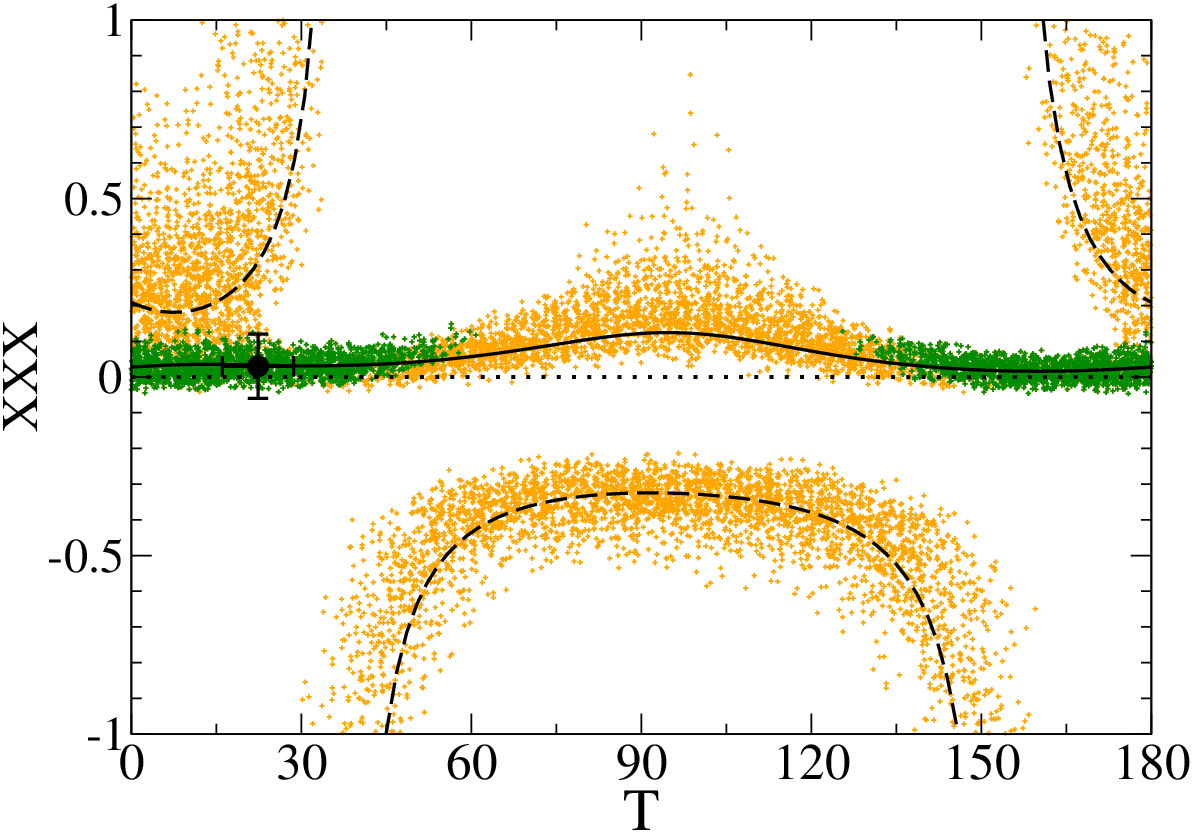
An alternative determination of these coefficients can be made using only the excited baryon masses, as discussed in Ref. [13]. In this paper it was shown that in any quark model containing only two-body quark interactions, the mixing angles are correlated (up to a discrete ambiguity) by Eq. (34) and by a second relation (Eq. (6) in Ref. [13]) expressing the spin-average of the singlet states in terms of the nonstrange states. Allowing for a conservative breaking correction of MeV in the relation for , we show in Fig. 1 the scatter plots for which impose the correlation Eq. (34) (all points), and also the relation for , satisfied on the dark shaded area (green points). The preferred solution is given by the solid line, which overlaps with the dark shaded area (green points).
We note that there is good agreement between the allowed values of the coefficients in the scatter plots and the results in Eq. (51), which are shown as the black point with error bars on the plot. Both these computations confirm the suppression of the coefficient relative to its natural size. The nonvanishing of can be related to a smearing out of the contact interaction. This is examined in the next Section, where it is also found that the sign of the ratio can provide information on the spin-flavor structure of the interaction.
III Finite range scalar quark interactions
In the general case of a finite range interaction, the orbital reduced matrix elements and are independent. According to Eq. (II) the coefficient will be in general nonvanishing, and proportional to the combination of the reduced matrix elements . The ratio of for the different spin-flavor structures can be expressed in terms of the ratio of reduced matrix elements
| (52) |
We start by considering the case when the quark Hamiltonian contains a single spin-flavor structure . For the pure OGE interaction the ratio of coefficients is predicted to be
| (53) |
For the GBE interaction with two light quark flavors , the coefficient is predicted to be exactly zero, independently of the spatial form of the quark interaction. With three light quark flavors , we have
| (54) |
Finally, for the isospin interaction , the ratio is
| (55) |
We will illustrate the effect of a finite range quark interaction by taking the spatial dependence of the interaction to be
| (56) |
with a coupling constant. Such an orbital dependence is generated by the exchange of a meson of mass [11], see Ref. [22] for a detailed derivation.
Adopting the functional form Eq. (56), we will assume that the contribution of the second term of to is always smaller than that of the first term. This is always satisfied if , where is defined by the squared wave function integrated over one of its arguments . Under this assumption, the contribution of the second term to any reduced matrix element is given by
| (57) |
and is thus smaller than the contribution of the first term. (In this example the quark interaction was taken between the quarks .) This proves that is always positive. Taking into account that the contribution to of the first term in Eq. (56) vanishes, it is easy to see that is negative and therefore the ratio of reduced matrix elements is negative.
The information about the sign of the ratio of reduced matrix elements is sufficiently predictive to distinguish between the models considered above, through the sign of the ratio of the coefficients , as shown in Table 3. We denoted here with OGEμ the vector meson exchange model corresponding to a vector meson or a constituent gluon with mass ; the limit corresponds to the usual one-gluon exchange (OGE) model.
| Model | sgn |
|---|---|
| OGEμ | |
| OGE | 0 |
| GBE | 0 |
| GBE | |
The natural size of the ratio is of order . Its very small value (see solid line in Fig. 2) cannot be explained by power counting in and must have a dynamical origin. We find that it is suppressed for pion exchange interactions in general (chiral limit or physical pion mass), as from the spin-flavor structure alone. In the case of gluon exchange interactions, its smallness is related to the spatial extent of the interaction (and not related to its spin-flavor structure as in the previous case). In the case of a contact spin-spin interaction and the ratio vanishes, but otherwise this ratio is different from zero.
We comment on the argument presented in Ref. [6] for the dominance of the operator in the mass operator, and compare it with our conclusions. As mentioned in the Introduction, in this paper it was argued that the dominance of the operator follows by assuming one pion exchange. This follows from the observation that one particular linear combination of operators is equivalent to the unit operator (taking its matrix element on the nonstrange states), up to corrections of
| (58) |
This identity allows one to eliminate one of the three scalar operators. Choosing to eliminate , the scalar part of the mass operator reads
| (59) |
For the pion exchange interaction (both contact and finite range) we find , which confirms the result of Ref. [6] of dominance of in the large limit. In our approach, at , the dominance of is exact for pion exchange or any contact interaction.
Using the numerical values of the coefficients from Eq. (51), the value of the ratio is
| (60) |
An alternative determination using only hadron masses is shown in Fig. 2. The solid line is the preferred solution [13] and gives a range of values compatible with the first determination (shown in Fig. 2 as the black point with error bars). The central value is positive and clearly suppressed with respect to its natural size for any value of the mixing angle . Its sign favors a pure vector boson exchange model OGEμ with a non-vanishing vector meson mass . However, within the errors, negative values or a vanishing ratio are also allowed, such that it is difficult to draw a clear conclusion. A more precise determination of the mixing angles and hadron masses may sharpen this determination and allow one to fix the sign of the ratio.
We comment briefly on the massive vector boson exchange model OGEμ, which produces a positive ratio . This corresponds to a massive gluon model, previously considered in the literature in Refs. [23, 24, 25, 26, 27]. In these works it has been suggested that, in the low energy limit, an effective gluon mass can be generated by nonperturbative QCD effects. In principle an effective gluon mass can be observed through its effect on the low energy limit of quark forces in the constituent quark model. In the next Section we perform a crude model calculation to give an estimate of the range of allowed values for the effective gluon mass .
The analysis presented above was limited to the spin-flavor structure of the scalar quark interaction. In the spin-orbit sector, it has been pointed out in Ref. [13] that the flavor dependent interactions are needed in order to reproduce the observed mass spectrum. Also in the tensor sector, flavor dependent operators are needed [7, 8] in order to produce a non-zero coefficient of the operator . Allowing for a mixture of all possible interactions with strengths
| (61) |
we get the following general results for the operator coefficients
| (62) | |||||
| (63) |
No simple conclusions about the relative contributions of the different spin-flavor interactions can be drawn in the most general case. For example, assuming a mixture of the OGE and GBE interactions (), it is possible to arrange positive values for by taking and sufficiently large relative to that the second term in dominates over the third one. It is interesting to notice that in the case of the simultaneous presence of a massless one gluon exchange interaction () and a finite range one pion exchange interaction the coefficient vanishes independently of their relative strengths.
IV Isgur-Karl model calculation
The finite range effects can be taken into account in a quantitative way by adopting a specific choice for the hadronic model. For illustration we consider the Isgur-Karl (IK) model [12], which has been widely used for describing the properties of the excited baryons. The matching of this model to the effective operator expansion has also been discussed in detail recently in Ref. [18].
The IK model describes three constituent quarks interacting by harmonic oscillator potentials
| (64) |
This Hamiltonian can be solved by introducing the reduced coordinates
| (65) |
Expressed in terms of , the Hamiltonian Eq. (64) has the form of two independent 3-dimensional oscillators
| (66) |
The eigenstates with orbital angular momentum are
| (67) | |||||
| (68) |
where .
The parameters of the model are [28]
| (69) |
The reduced matrix elements are given by the matrix elements
| (70) | |||
| (71) |
The combination of reduced matrix elements was computed in Ref. [18] (see Eq. (52)) in the limit of a contact interaction . Using the spatial dependence of given in Eq. (56) one finds the complete result for
| (72) |
where the function is given by
| (73) |
and is positive for , which confirms that the contribution of the finite range term in is never larger than that of the contact term.
The function is the cumulative normal distribution function, which is related to the erf function, and is defined as
| (74) |
In a similar way one can compute also the combination of reduced matrix elements which vanishes in the limit of a contact interaction. We obtain
| (75) |
where the function is given by
| (76) |
and is positive for .
The asymptotic behavior of the functions at small and large values of the argument is
| (77) | |||||
| (78) | |||||
| (79) | |||||
| (80) |
The unknown constant cancels out in the ratio of reduced matrix elements , which depends only on the ratio
| (81) |
We show in Fig. 3 a plot of the ratio as a function of . The ratio vanishes in the limit of a massless exchanged particle, while for an infinitely heavy mass it approaches a finite limit .

Using these results we can obtain constraints on the mass of the exchanged boson. We quote results separately for the negative and positive ranges of the ratio , corresponding to the and OGEμ models 33 3 For a negative ratio we also have the GBE (F=3) interaction, but we don’t consider it in the phenomenological discussion as flavor is broken., respectively. From Eq. (51) one finds
Using Eq. (81) this can be translated into ranges of allowed values for the boson mass , namely
| (85) |
Using for the mass scale the typical value of the Isgur-Karl model given in Eq. (69), we obtain for the mass of the vector boson which can reproduce the observed data the allowed range MeV. This is much smaller than the lowest bound for a constituent gluon mass MeV suggested by lattice calculations of hybrid meson masses [29] and the glueball spectrum [30]. The use of the Isgur-Karl model and its parameters is a very crude first attempt to give an estimate of in the OGEμ case. It would be worthwhile to improve on this to see if it is possible to obtain a better estimate of that is compatible with the bounds obtained from lattice calculations, as well as an interpretation of the other possible spin-flavor interactions as the result of quark exchange or meson exchange interactions.
V Summary and conclusions
The hierarchy of the observed coefficients in the expansion for the excited baryons has a very specific pattern, with one of the subleading operator dominating, and the coefficients of the other operators suppressed. In this paper we present a possible explanation for the dominance of the operator in the framework of the constituent quark model.
Considering the most general two-body quark interaction, we show that a contact quark interaction leads to the suppression of certain coefficients in the operator expansion. Furthermore, any spin-flavor zero range two-body quark interaction is matched onto the same operator . Intuitively, this can be understood from the fact that the excited and core quarks are in a relative p-wave, and thus the coefficients of and vanish if the spatial part of the interaction is a function [7]. This result implies that it is impossible to distinguish between different models of quark interactions as long as they are of zero range.
Allowing for a quark interaction of finite range, modeled by the exchange of a particle of mass , we study the question of obtaining information about the spin-flavor structure of the scalar part of the quark interaction from the mass spectrum of the negative parity excited baryons. Under the assumption that only one spin-flavor structure dominates, we find that the sign of the ratio , that can be obtained from the experimental masses and mixing angles, can be used as a test of the spin-flavor structure of the interaction.
The central value we obtain for this ratio corresponds to a spin-spin interaction with the exchange of a massive vector boson. Using the wave functions of the Isgur-Karl model, the mass of the exchanged vector meson is in the range MeV, which is much smaller than the lowest bound for the mass of a constituent gluon, as suggested by lattice calculations of hybrid meson masses [29] and glueballs [30]. This seems to disfavor this type of interaction. The present study shows that within error bars and allowing for two scalar spin-flavor structures, the one (massless) gluon exchange and the one pion exchange interactions lead to independently of their relative strengths, and are consistent with data. Previous studies [7, 8, 13] that did not focus on the range of the microscopic interaction also include the spin-orbit and tensor terms, and suggest that both gluon exchange and flavor dependent interactions are needed to reproduce the data. Allowing for a more general combination of spin-flavor structures and finite range forces, no useful information on their contribution is obtained from the present analysis in the absence of additional dynamical information about their relative strength.
Acknowledgements.
The work of C.S. was supported by CONICET and partially supported by the U. S. Department of Energy, Office of Nuclear Physics under contract No. DE-FG02-93ER40756 with Ohio University.References
- [1] D. Pirjol and C. Schat, arXiv:0711.2006 [hep-ph]. J. Goity, talk at the XIII International Conference on Hadron Spectroscopy, Florida, 2009.
- [2] C. Carone, H. Georgi and S. Osofsky, Phys. Lett. B 322, 227 (1994) [arXiv:hep-ph/9310365].
- [3] M. A. Luty and J. March-Russell, Nucl. Phys. B 426, 71 (1994) [arXiv:hep-ph/9310369].
- [4] R. F. Dashen, E. E. Jenkins and A. V. Manohar, Phys. Rev. D 51, 3697 (1995) [arXiv:hep-ph/9411234].
- [5] J. L. Goity, Phys. Lett. B 414, 140 (1997) [arXiv:hep-ph/9612252].
- [6] C. E. Carlson, C. D. Carone, J. L. Goity and R. F. Lebed, Phys. Rev. D 59, 114008 (1999) [arXiv:hep-ph/9812440].
- [7] C. L. Schat, J. L. Goity and N. N. Scoccola, Phys. Rev. Lett. 88, 102002 (2002) [arXiv:hep-ph/0111082].
- [8] J. L. Goity, C. L. Schat and N. N. Scoccola, Phys. Rev. D 66, 114014 (2002) [arXiv:hep-ph/0209174].
- [9] A. De Rujula, H. Georgi and S. L. Glashow, Phys. Rev. D 12, 147 (1975).
- [10] R. L. Jaffe, Phys. Rev. D 15, 281 (1977).
- [11] L. Y. Glozman and D. O. Riska, Phys. Rept. 268, 263 (1996) [arXiv:hep-ph/9505422].
- [12] N. Isgur and G. Karl, Phys. Lett. B 72, 109 (1977); Phys. Rev. D 18, 4187 (1978).
- [13] D. Pirjol and C. Schat, Phys. Rev. Lett. 102, 152002 (2009) [arXiv:0811.1345 [hep-ph]].
- [14] D. Pirjol and C. Schat, Phys. Rev. D 78, 034026 (2008) [arXiv:0709.0714 [hep-ph]].
- [15] H. Collins and H. Georgi, Phys. Rev. D 59, 094010 (1999) [arXiv:hep-ph/9810392].
- [16] C. Semay, F. Buisseret, N. Matagne and F. Stancu, Phys. Rev. D 75, 096001 (2007) [arXiv:hep-ph/0702075].
- [17] C. Semay, F. Buisseret and F. Stancu, Phys. Rev. D 76, 116005 (2007) [arXiv:0708.3291 [hep-ph]].
- [18] L. Galeta, D. Pirjol and C. Schat, Phys. Rev. D 80, 116004 (2009) [arXiv:0906.0699 [hep-ph]].
- [19] J. L. Goity, C. Schat and N. Scoccola, Phys. Rev. D 71, 034016 (2005) [arXiv:hep-ph/0411092].
- [20] N. N. Scoccola, J. L. Goity and N. Matagne, Phys. Lett. B 663, 222 (2008) [arXiv:0711.4203 [hep-ph]].
- [21] C. Amsler et al. [Particle Data Group], Phys. Lett. B 667, 1 (2008).
- [22] J. Eiglsperger, arXiv:0707.1269 [hep-ph].
- [23] J. M. Cornwall, Phys. Rev. D 26, 1453 (1982).
- [24] J. E. Mandula, Phys. Rept. 315, 273 (1999) [arXiv:hep-lat/9907020].
- [25] R. Alkofer and L. von Smekal, Phys. Rept. 353, 281 (2001) [arXiv:hep-ph/0007355].
- [26] V. Mathieu, N. Kochelev and V. Vento, Int. J. Mod. Phys. E 18, 1 (2009) [arXiv:0810.4453 [hep-ph]].
- [27] J. M. Cornwall and A. Soni, Phys. Lett. B 120, 431 (1983).
- [28] S. Capstick and W. Roberts, Prog. Part. Nucl. Phys. 45, S241 (2000) [arXiv:nucl-th/0008028].
- [29] C. Bernard et al., Phys. Rev. D 68, 074505 (2003) [arXiv:hep-lat/0301024].
- [30] Y. Chen et al., Phys. Rev. D 73, 014516 (2006) [arXiv:hep-lat/0510074].