跳到论文正文
W Papers独立论文阅读器 arXiv:1007.0950 论文正文 计算阅读时间 · 0%
引用这篇论文根据当前论文元数据生成,正式投稿前建议核对。


License: arXiv.org perpetual non-exclusive license
arXiv:1007.0950v2 [math.AP] 06 Sep 2010

Spreading speeds and traveling waves for non-cooperative reaction-diffusion systems Thanks: This manuscript is available at arXiv:1007.0950

Haiyan Wang Address: Division of Mathematical and Natural Sciences
Arizona State University
Phoenix, AZ 85069-7100, USA
Email: wangh@asu.edu
Abstract

Much has been studied on the spreading speed and traveling wave solutions for cooperative reaction-diffusion systems. In this paper, we shall establish the spreading speed for a large class of non-cooperative reaction-diffusion systems and characterize the spreading speed as the slowest speed of a family of non-constant traveling wave solutions. As an application, our results are applied to a partially cooperative system describing interactions between ungulates and grass.

Keywords: 
traveling waves, non-cooperative systems, spreading speed, reaction-diffusion systems
MSC
Primary: 35K45, 35K57, 35B40; Secondary: 92D25, 92D40

1 Introduction

Fisher [11] studied the nonlinear parabolic equation

wt=wx​x+w⁡(1−w).w_{t}=w_{xx}+w(1-w). (1.1)

for the spatial spread of an advantageous gene in a population and conjectured c∗c^{*} is the asymptotic speed of propagation of the advantageous gene. His results show that (1.1) has a traveling wave solution of the form w⁡(x+c​t)w(x+ct) if only if |c|≥c∗=2.|c|\geq c^{*}=2. Kolmogorov, Petrowski, and Piscounov [16] proved the similar results with more general model. Those pioneering work along with the paper by Aronson and Weinberger [1, 2] confirmed the conjecture of Fisher and established the speeding spreads for nonlinear parabolic equations. Lui [20] established the theory of spreading speeds for cooperative recursion systems. In a series of papers, Weinberger, Lewis and Li [17, 18, 32, 33] studied spreading speeds and traveling waves for more general cooperative recursion systems, and in particular, for quite general cooperative reaction-diffusion systems by analyzing of traveling waves and the convergence of initial data to wave solutions.

However, due to various biological or physical constrains, many reaction-diffusion systems are not necessarily cooperative. Thieme [27] showed that asymptotic spreading speed of a model with nonmonotone growth functions can still be obtained by constructing monotone functions. Weinberger, Kawasaki and Shigesada [36] discussed the reaction-diffusion model

∂u1∂t=d1​Δ​u1+u1​[−α−δ​u1+r1​u2]∂u2∂t=d2​Δ​u2+u2​r2​[1−u2+h⁡(u1)]\begin{split}\frac{\partial u_{1}}{\partial t}&=d_{1}\Delta u_{1}+u_{1}[-\alpha-\delta u_{1}+r_{1}u_{2}]\\ \frac{\partial u_{2}}{\partial t}&=d_{2}\Delta u_{2}+u_{2}r_{2}[1-u_{2}+h(u_{1})]\\ \end{split} (1.2)

where d1,α,δ,r1,d2,r2d_{1},\alpha,\delta,r_{1},d_{2},r_{2} are all positive parameters. This system describes the interaction between ungulates with linear density u1​(x,t)u_{1}(x,t) and grass with linear density u2​(x,t).u_{2}(x,t). The function h⁡(u1)h(u_{1}) models the increase in the specific growth rate of the grass due to the presence of ungulates. When the density u1u_{1} is small the net effect of ungulates is increasingly beneficial, but as the density increases above a certain value, the benefits decrease with increasing u1u_{1}. (1.2) is partially cooperative 2-species reaction-diffusion model, meaning that it is cooperative for small population densities but not for large ones. By employing comparison methods [36] established spreading speeds for (1.2). In Section 5, we take the non-monotone Ricker function u1​e−u1u_{1}e^{-u_{1}} as h⁡(u1)h(u_{1}), which is simpler than that of [36], and apply our main theorem (Theorem 2.1) to (1.2). The application of our general theorem allows us to characterize the spreading speed as the slowest speed of traveling wave solutions to (1.2), which is new and was not proved in [36]. Non-cooperative reaction-diffusion systems frequently occur in other biological systems such as epidermal wound healing (see, Sherratt and Murray [25, 26], Dale, Maini, Sherratt [7]). In a recent paper by the author [31], spreading speeds and traveling waves for a non-cooperative reaction-diffusion model of epidermal wound healing were established.

For related non-monotone integro-difference equations, Hsu and Zhao [14], Li, Lewis and Weinberger [19] extended the theory of spreading speed and established the existence of travel wave solutions. The author and Castillo-Chavez [30] prove that a large class of nonmonotone integro-difference systems have spreading speeds and traveling wave solutions. Such an extension is largely based on the construction of two monotone operators with appropriate properties and fixed point theorems in Banach spaces. A similar method was also used in Ma [23] and the author [29] to prove the existence of traveling wave solutions of nonmonotone reaction-diffusion equations.

In this paper, we shall establish the spreading speed for a general non-cooperative system (1.3) and characterize its spread speed as the slowest speed of a family of non-constant traveling wave solutions of (1.3). Our main theorem (Theorem 2.1) will be applied to (1.2) in Section 5.

We begin with some notation. We shall use R,k,k±,f,f±,r,u,vR,k,k^{\pm},f,f^{\pm},r,u,v to denote vectors in ℝN\mathbb{R}^{N} or NN-vector valued functions , and x,y,ξx,y,\xi the single variable in ℝ\mathbb{R}. Let u=(ui),v=(vi)∈ℝNu=(u_{i}),v=(v_{i})\in\mathbb{R}^{N}, we write u≥vu\geq v if ui≥viu_{i}\geq v_{i} for all ii; and u≫vu\gg v if ui>viu_{i}>v_{i} for all ii. A vector uu is positive if u≫0u\gg 0. For any r=(ri)≫0,r∈ℝNr=(r_{i})\gg 0,r\in\mathbb{R}^{N} let

[0,r]={u:0≤u≤r,u∈ℝN}⊆ℝN[0,r]=\{u:0\leq u\leq r,u\in\mathbb{R}^{N}\}\subseteq\mathbb{R}^{N}

and

𝒞r={u=(ui):ui∈C(ℝ,ℝ),0≤ui(x)≤ri,x∈ℝ,i=1,…,N},\mathcal{C}_{r}=\{u=(u_{i}):u_{i}\in C(\mathbb{R},\mathbb{R}),0\leq u_{i}(x)\leq r_{i},x\in\mathbb{R},\;i=1,...,N\},

where C⁡(ℝ,ℝ)C(\mathbb{R},\mathbb{R}) is the set of all continuous functions from ℝ\mathbb{R} to ℝ\mathbb{R}.

Consider the system of reaction-diffusion equations

ut=D​ux​x+f⁡(u),x∈ℝ,t≥0.u_{t}=Du_{xx}+f(u),x\in\mathbb{R},\;t\geq 0. (1.3)

with

u⁡(x,0)=u0​(x),x∈ℝ,u(x,0)=u_{0}(x),\;\;x\in\mathbb{R}, (1.4)

where u=(ui)u=(u_{i}), D=diag(d1,d2,…,dN),di>0,i=1,…,ND=\text{diag}(d_{1},d_{2},...,d_{N}),d_{i}>0,i=1,...,N

f⁡(u)=(f1​(u),f2​(u),…,fN​(u)),f(u)=(f_{1}(u),f_{2}(u),...,f_{N}(u)),

u0​(x)u_{0}(x) is a bounded uniformly continuous function on ℝ.\mathbb{R}. In this paper, by a solution we mean a twice continuously differentiable function uu satisfying appropriate equation in ℝ\mathbb{R} and an initial condition.

In order to deal with non-cooperative system, we shall assume that there are additional two monotone operators f±f^{\pm}, one lies above and another below ff with the corresponding equations

ut=D​ux​x+f+​(u),x∈ℝ,t≥0.u_{t}=Du_{xx}+f^{+}(u),x\in\mathbb{R},\;t\geq 0. (1.5)
ut=D​ux​x+f−​(u),x∈ℝ,t≥0.u_{t}=Du_{xx}+f^{-}(u),x\in\mathbb{R},\;t\geq 0. (1.6)

Such an assumption will enable us to make use of the corresponding results for cooperative systems in [20, 32] to establish spreading speeds for (1.3).

  1. (H1)
    • i.

      Let k+=(ki+)>>0k^{+}=(k^{+}_{i})>>0 and f:[0,k+]→ℝNf:[0,k^{+}]\to\mathbb{R}^{N} be a continuous and twice piecewise continuous differentiable function. Assume that 𝒞k+\mathcal{C}_{k^{+}} is an invariant set of (1.3) in the sense that for any given u0∈𝒞k+u_{0}\in\mathcal{C}_{k^{+}}, the solution of (1.3) with the initial condition u0u_{0} exists and remains in 𝒞k+\mathcal{C}_{k^{+}} for t∈[0,∞)t\in[0,\infty).

    • ii.

      Let 0<<k−=(ki−)≤k=(ki)≤k+.0<<k^{-}=(k^{-}_{i})\leq k=(k_{i})\leq k^{+}. Assume there exist continuous and twice piecewise continuous differentiable function f±=(fi±):[0,k+]→ℝNf^{\pm}=(f^{\pm}_{i}):[0,k^{+}]\to\mathbb{R}^{N} such that for u∈[0,k+]u\in[0,k^{+}]

      f−​(u)≤f⁡(u)≤f+​(u).f^{-}(u)\leq f(u)\leq f^{+}(u).
    • iii.

      f⁡(0)=f⁡(k)=0f(0)=f(k)=0 and there is no other positive equilibrium of ff between 00 and kk. f±​(0)=f±​(k±)=0f^{\pm}(0)=f^{\pm}(k^{\pm})=0. There is no other positive equilibrium of f±f^{\pm} between 00 and k±k^{\pm}.

    • iv.

      (1.5) and (1.6) are cooperative (i.e. ∂ifj±​(u)≥0\partial_{i}f^{\pm}_{j}(u)\geq 0 for u∈[0,k±],i≠ju\in[0,k^{\pm}],i\neq j). f±​(u),f​(u)f^{\pm}(u),f(u) have the same Jacobian matrix f′​(0)f^{\prime}(0) at u=0u=0.

A traveling wave solution uu of (1.3) is a solution of the form u=u⁡(x+c​t),u∈C⁡(ℝ,ℝN)u=u(x+ct),u\in C(\mathbb{R},\mathbb{R}^{N}) . Substituting u⁡(x,t)=u⁡(x+c​t)u(x,t)=u(x+ct) into (1.3) and letting ξ=x+c​t\xi=x+ct, we obtain the wave equation

D​u′′​(ξ)−c​u′​(ξ)+f⁡(u⁡(ξ))=0,ξ∈ℝ.Du^{\prime\prime}(\xi)-cu^{\prime}(\xi)+f(u(\xi))=0,\;\;\xi\in\mathbb{R}. (1.7)

Now if we look for a solution of the form (ui)=(eλ​ξ​ηλi),λ>0,ηλ=(ηλi)>>0(u_{i})=\big(e^{\lambda\xi}\eta^{i}_{\lambda}\big),\lambda>0,\eta_{\lambda}=(\eta^{i}_{\lambda})>>0 for the linearization of (1.7) at the origin, we arrive at the following system equation

diag​(di​λ2−c​λ)​ηλ+f′​(0)​ηλ=0\text{diag}(d_{i}\lambda^{2}-c\lambda)\eta_{\lambda}+f^{\prime}(0)\eta_{\lambda}=0

which can be rewritten as the following eigenvalue problem

1λ​Aλ​ηλ=c​ηλ,\frac{1}{\lambda}A_{\lambda}\mathbf{\eta_{\lambda}}=c\mathbf{\eta_{\lambda}}, (1.8)

where

Aλ=(aλi,j)=diag​(di​λ2)+f′​(0)A_{\lambda}=(a^{i,j}_{\lambda})=\text{diag}(d_{i}\lambda^{2})+f^{\prime}(0)

The matrix f′​(0)f^{\prime}(0) has nonnegative off diagonal elements. In fact, there is a constant α\alpha such that f′​(0)+α​If^{\prime}(0)+\alpha I has nonnegative entries, where II is the identity matrix.

By reordering the coordinates, we can assume that f′​(0)f^{\prime}(0) is in block lower triangular form, in which all the diagonal blocks are irreducible or 11 by 11 zero matrix. A matrix is irreducible if it is not similar to a lower triangular block matrix with two blocks via a permutation. From the Perron-Frobenius theorem any irreducible matrix AA with nonnegative entries has a unique principal positive eigenvalue( which is the spectral radius of AA, ρ⁡(A)\rho(A)) with a corresponding principal eigenvector with strictly positive coordinates. For an irreducible matrix AA with nonnegative off diagonal elements, we shall call the eigenvalue ρ⁡(A+α​I)−α\rho(A+\alpha I)-\alpha of AA, which has the same positive eigenvector, the principal eigenvalue of AA (see e.g. [13, 32]). Let

Ψ⁡(A)=ρ⁡(A+α​I)−α.\Psi(A)=\rho(A+\alpha I)-\alpha.

Here A+α​IA+\alpha I is irreducible and nonnegative, and ρ⁡(A+α​I)\rho(A+\alpha I) is the spectral radius of A+α​I.A+\alpha I.

We shall need the following assumption (H2). Notice that (H2) is assumed for λ=0\lambda=0 in [32]. However, with (H2), we are able to obtain better estimates for traveling solutions and the minimum speed c∗c^{*}, see Lemma 1.1. As a result, for the example in Section 5, a slightly stronger assumption (d1≥d2d_{1}\geq d_{2}) than [36] is be assumed.

  1. (H2)
    • Assume that, for each λ>0\lambda>0, AλA_{\lambda} is in block lower triangular form and the first diagonal block has the positive principal eigenvalue Ψ⁡(Aλ)\Psi(A_{\lambda}), and Ψ⁡(Aλ)\Psi(A_{\lambda}) is strictly larger than the principal eigenvalues of all other diagonal blocks, and that there is a positive eigenvector νλ=(νλi)>>0\nu_{\lambda}=(\nu^{i}_{\lambda})>>0 of AλA_{\lambda} corresponding to Ψ⁡(Aλ)\Psi(A_{\lambda}). And further assume that νλ\nu_{\lambda} is continuous with respect to λ.\lambda.

Let

Φ⁡(λ)=1λ​Ψ​(Aλ)>0.\Phi(\lambda)=\frac{1}{\lambda}\Psi(A_{\lambda})>0.
Refer to caption
Figure 1: The red curve is Φ⁡(λ)\Phi(\lambda). The minimum of Φ⁡(λ)\Phi(\lambda) is c∗c^{*}. For c>c∗c>c^{*}, the left solution of Φ⁡(λ)=c\Phi(\lambda)=c is Λc\Lambda_{c}.

According to Lemma 1.1, we can expect the graph of Φ\Phi as in Fig. 1. For the example in Section 5, Φ\Phi is a strictly convex function of λ\lambda and, clearly satisfies Lemma 1.1.

Now we state Lemma 1.1, which shall enable us to give accurate asymptotic estimates of traveling solutions. Lemma 1.1 is a analogous result in Weinberger [35] and Lui [20]. However, due to the fact that f′​(0)f^{\prime}(0) is only quasi-positive and the elements of AλA_{\lambda} are not necessarily log convex, some of its proofs here are different from Lui [20]. A theorem on the convexity of the dominant eigenvalue of matrices due to Cohen [5] is used to show that Ψ⁡(Aλ)\Psi(A_{\lambda}) is convex function of λ\lambda.

There are two direct consequences of Lemma 1.1. First one, it improves [32, Theorem 4.2], which will be used in this paper, by eliminating the case (b) in [32, Theorem 4.2] because of Lemma 1.1 (7). Second, Lemma 1.1 (8) will allow us to construct explicit lower solutions and therefore asymptotic behavior of traveling solutions of (1.3) can be obtained.

Lemma 1.1

Assume that (H​1)−(H​2)(H1)-(H2) hold. Then

  1. (1)

    Φ⁡(λ)→∞\Phi(\lambda)\to\infty as λ→0;\lambda\to 0;

  2. (2)

    Φ⁡(λ)→∞\Phi(\lambda)\to\infty as λ→∞;\lambda\to\infty;

  3. (3)

    Φ⁡(λ)\Phi(\lambda) is decreasing as λ=0+;\lambda=0^{+};

  4. (4)

    Ψ⁡(Aλ)\Psi(A_{\lambda}) is a convex function of λ>0;\lambda>0;

  5. (6)

    Φ′​(λ)\Phi^{\prime}(\lambda) changes sign at most once on (0,∞)(0,\infty)

  6. (7)

    Φ⁡(λ)\Phi(\lambda) has the minimum

    c∗=infλ>0Φ⁡(λ)>0c^{*}=\inf_{\lambda>0}\Phi(\lambda)>0

    at a finite λ\lambda.

  7. (8)

    For each c>c∗c>c^{*}, there exist Λc>0\Lambda_{c}>0 and γ∈(1,2)\gamma\in(1,2) such that

    Φ⁡(Λc)=c,Φ⁡(γ​Λc)<c.\Phi(\Lambda_{c})=c,\;\;\Phi(\gamma\Lambda_{c})<c.

    That is

    1Λc​AΛc​νΛc=Φ⁡(Λc)​νΛc=c​νΛc\frac{1}{\Lambda_{c}}A_{\Lambda_{c}}\nu_{\Lambda_{c}}=\Phi(\Lambda_{c})\nu_{\Lambda_{c}}=c\nu_{\Lambda_{c}}

    and

    1γ​Λc​Aγ​Λc​νγ​Λc=Φ⁡(γ​Λc)​νγ​Λc<c​νγ​Λc\frac{1}{\gamma\Lambda_{c}}A_{\gamma\Lambda_{c}}\nu_{\gamma\Lambda_{c}}=\Phi(\gamma\Lambda_{c})\nu_{\gamma\Lambda_{c}}<c\nu_{\gamma\Lambda_{c}}

    where νΛc>>0,νγ​Λc>>0\nu_{\Lambda_{c}}>>0,\nu_{\gamma\Lambda_{c}}>>0 are positive eigenvectors of 1Λc​AΛc,1γ​Λc​Aγ​Λc\frac{1}{\Lambda_{c}}A_{\Lambda_{c}},\frac{1}{\gamma\Lambda_{c}}A_{\gamma\Lambda_{c}} corresponding to eigenvalues Φ⁡(Λc)\Phi(\Lambda_{c}) and Φ⁡(γ​Λc)\Phi(\gamma\Lambda_{c}) respectively.

{@proof}

[Proof.]We only need to prove those different from [35, 20]. The proof of the convexity of Ψ⁡(Aλ)\Psi(A_{\lambda}) is similar to that in Crooks [6] for matrices with positive off-diagonal elements. It is easily seen that Ψ⁡(Aλ)=ρ⁡(Aλ+α​I)−α\Psi(A_{\lambda})=\rho(A_{\lambda}+\alpha I)-\alpha is non-decreasing function of λ>0\lambda>0 ([13, Theorem 8.1.18]). Further, a theorem on the convexity of the dominant eigenvalue of matrices due to Cohen [5] states that for any positive diagonal matrices D1,D2D_{1},D_{2} and t∈(0,1)t\in(0,1),

Ψ⁡(t​D1+(1+t)​D2+f′​(0))≤t​Ψ​(D1+f′​(0))+(1−t)​Ψ​(D2+f′​(0))\Psi(tD_{1}+(1+t)D_{2}+f^{\prime}(0))\leq t\Psi(D_{1}+f^{\prime}(0))+(1-t)\Psi(D_{2}+f^{\prime}(0))

As before Ψ⁡(A)\Psi(A) is the principle eigenvalue of AA. Now if α1,α2∈ℝ\alpha_{1},\alpha_{2}\in\mathbb{R} and t∈(0,1)t\in(0,1),

(t​α1+(1−t)​α2)2≤t​α12+(1−t)​α22.(t\alpha_{1}+(1-t)\alpha_{2})^{2}\leq t\alpha_{1}^{2}+(1-t)\alpha_{2}^{2}.

This implies that

Ψ⁡(At​λ1+(1−t)​λ2)=Ψ⁡((t​λ1+(1−t)​λ2)2​D+f′​(0))≤Ψ⁡(t​λ12​D+(1−t)​λ22​D+f′​(0))≤t​Ψ​(λ12​D+f′​(0))+(1−t)​Ψ​(λ22​D+f′​(0))=t​Ψ​(Aλ1)+(1−t)​Ψ​(Aλ2)\begin{split}\Psi(A_{t\lambda_{1}+(1-t)\lambda_{2}})&=\Psi((t\lambda_{1}+(1-t)\lambda_{2})^{2}D+f^{\prime}(0))\\ &\leq\Psi(t\lambda_{1}^{2}D+(1-t)\lambda_{2}^{2}D+f^{\prime}(0))\\ &\leq t\Psi(\lambda_{1}^{2}D+f^{\prime}(0))\\ &\quad+(1-t)\Psi(\lambda_{2}^{2}D+f^{\prime}(0))\\ &=t\Psi(A_{\lambda_{1}})+(1-t)\Psi(A_{\lambda_{2}})\\ \end{split}

Since Ψ⁡(Aλ)\Psi(A_{\lambda}) is a simple root of the characteristic equation of an irreducible block, it can be shown that Ψ⁡(Aλ)\Psi(A_{\lambda}) is twice continuously differentiable on ℝ\mathbb{R}. Thus

Ψ′′​(λ)≥0\Psi^{\prime\prime}(\lambda)\geq 0

and a calculation shows

[λ​Φ​(λ)]′=Ψ′​(λ)[\lambda\Phi(\lambda)]^{\prime}=\Psi^{\prime}(\lambda)
Φ′​(λ)=1λ​[Ψ′​(λ)−Φ⁡(λ)]\Phi^{\prime}(\lambda)=\frac{1}{\lambda}[\Psi^{\prime}(\lambda)-\Phi(\lambda)]

and

(λ2​Φ′​(λ))′=λ​Ψ′′​(λ)≥0.(\lambda^{2}\Phi^{\prime}(\lambda))^{\prime}=\lambda\Psi^{\prime\prime}(\lambda)\geq 0.

(6) is a consequence of the above inequalities. As for (2), we need to prove that limλ→∞Ψ⁡(Aλ)λ=∞\lim_{\lambda\to\infty}\frac{\Psi(A_{\lambda})}{\lambda}=\infty. In fact, there exists an ϵ>0\epsilon>0 such that all diagonal elements of D−ϵ​ID-\epsilon I are strictly positive, then Ψ⁡(D−ϵ​I)>0\Psi\big(D-\epsilon I\big)>0 and choose λ\lambda large enough so that

Ψ⁡(Aλ)=Ψ⁡(D​λ2+f′​(0))=Ψ⁡((D−ϵ​I)​λ2+(ϵ​λ2​I+f′​(0)))≥Ψ⁡((D−ϵ​I)​λ2)=λ2​Ψ​(D−ϵ​I)\begin{split}\Psi(A_{\lambda})&=\Psi(D\lambda^{2}+f^{\prime}(0))\\ &=\Psi\big((D-\epsilon I)\lambda^{2}+(\epsilon\lambda^{2}I+f^{\prime}(0))\big)\\ &\geq\Psi\big((D-\epsilon I)\lambda^{2}\big)\\ &=\lambda^{2}\Psi\big(D-\epsilon I\big)\end{split}

Thus limλ→∞Ψ⁡(Aλ)λ=∞\lim_{\lambda\to\infty}\frac{\Psi(A_{\lambda})}{\lambda}=\infty. As we discussed before, (H2) implies the existence of positive eigenvector νλ>>0\nu_{\lambda}>>0 corresponding to Φ⁡(Aλ)\Phi(A_{\lambda}). The first statement of (8) is a consequence of (1)-(7). The second statement of (8) is just a rephrase of the fact that νλ>>0\nu_{\lambda}>>0 is a eigenvector of 1λ​Aλ\frac{1}{\lambda}A_{\lambda} corresponding to eigenvalue Φ⁡(Aλ)\Phi(A_{\lambda}) for λ=Λc\lambda=\Lambda_{c} and γ​Λc\gamma\Lambda_{c}.

□\quad\Box

In addition to (H1-H2), we also need assumption (H3) which only requires the nonlinearity grow less than its linearization along the particular function νλ​e−λ​x\nu_{\lambda}e^{-\lambda x} [32]. Such a condition can be satisfied for many biological systems.

  1. (H3)
    • Assume that for any α>0,λ>0\alpha>0,\lambda>0

      f±​(α​νλ)≤α​f′​(0)​νλ,where​νλ=(νλi).f^{\pm}(\alpha\nu_{\lambda})\leq\alpha f^{\prime}(0)\nu_{\lambda},\;\;\text{where}\;\;\nu_{\lambda}=(\nu^{i}_{\lambda}).

We now recall results on the spreading speeds in Weinberger, Lewis and Li [32] and Lui [20]. While Theorem 4.1 [32] holds for non cooperative reaction-diffusion systems, it does require that the reaction-diffusion system has a single speed. In general, such a condition is very difficult to verify. In the same section, for cooperative systems, Theorem 4.2 in [32] provides sufficient conditions to have a single speed. The following theorem combines the results of Theorems 4.1 and 4.2 in [32], which can be a consequence of Theorems 3.1 and 3.2 for discrete-time recursions in Lui [20].

Theorem 1.2

(Weinberger, Lewis and Li [32]) Assume (H​1)−(H​3)(H1)-(H3) hold and (1.3) is cooperative. Then the following statements are valid:

  1. (i)

    For any u0∈𝒞ku_{0}\in\mathcal{C}_{k} with compact support, let u⁡(x,t)u(x,t) be the solution of (1.3) with (1.4). Then

    limt→∞sup|x|≥c​tu⁡(x,t)=0, for ​c>c∗\lim_{t\to\infty}\sup_{\lvert x\rvert\geq ct}u(x,t)=0,\text{ for }c>c^{*}
  2. (ii)

    For any strictly positive vector ω∈ℝN\omega\in\mathbb{R}^{N}, there is a positive RωR_{\omega} with the property that if u0∈𝒞ku_{0}\in\mathcal{C}_{k} and u0≥ωu_{0}\geq\omega on an interval of length 2​Rω2R_{\omega}, then the solution u⁡(x,t)u(x,t) of (1.3) with (1.4) satisfies

    lim inft→∞inf|x|≤t​cu⁡(x,t)=k, for ​0<c<c∗\liminf_{t\to\infty}\inf_{\lvert x\rvert\leq tc}u(x,t)=k,\text{ for }0<c<c^{*}

In another paper [18], for cooperative systems, Li, Weinberger and Lewis established that the slowest spreading speed c∗c^{*} can always be characterized as the slowest speed of a family of traveling waves. These results describe the properties of spreading speed c∗c^{*} for monotone systems. Based on these spreading results for cooperative systems, we will discuss analogous spreading speed results for non cooperative systems.

2 Main Results

Our new contributions in this paper are to establish the spreading speed (Theorem 2.1 (i-ii)) for general non-cooperative reaction-diffusion systems (1.3), and further characterize the spreading speed as the speed of the slowest non-constant traveling wave solutions (Theorem 2.1 (iii-v)).

Although the existence of traveling wave solutions for cooperative systems are known (see,e.g. [18]), we shall prove the existence of traveling wave solutions for both cooperative and non cooperative systems as our proofs for non cooperative systems are based on those for cooperative systems. Further, in additions to the existence of traveling wave solutions, we shall be able to obtain asymptotic behavior of the traveling wave solutions in terms of eigenvalues and eigenvectors for both cooperative and non cooperative systems. The following theorem is our main results.

Theorem 2.1

Assume (H​1)−(H​3)(H1)-(H3) hold. Then the following statements are valid:

  1. (i.)

    For any u0∈𝒞ku_{0}\in\mathcal{C}_{k} with compact support, the solution u⁡(x,t)u(x,t) of (1.3) with (1.4) satisfies

    limt→∞sup|x|≥t​cu⁡(x,t)=0, for ​c>c∗\lim_{t\to\infty}\sup_{\lvert x\rvert\geq tc}u(x,t)=0,\text{ for }c>c^{*}
  2. (ii.)

    For any vector ω∈ℝN,ω>>0\omega\in\mathbb{R}^{N},\omega>>0, there is a positive RωR_{\omega} with the property that if u0∈𝒞ku_{0}\in\mathcal{C}_{k} and u0≥ωu_{0}\geq\omega on an interval of length 2​Rω2R_{\omega}, then the solution u⁡(x,t)u(x,t) of (1.3) with (1.4) satisfies

    k−≤lim inft→∞inf|x|≤t​cu⁡(x,t)≤k+, for ​0<c<c∗k^{-}\leq\liminf_{t\to\infty}\inf_{\lvert x\rvert\leq tc}u(x,t)\leq k^{+},\text{ for }0<c<c^{*}
  3. (iii.)

    For each c>c∗c>c^{*} (1.3) admits a traveling wave solution u=u⁡(x+c​t)u=u(x+ct) such that 0<<u⁡(ξ)≤k+,ξ∈ℝ0<<u(\xi)\leq k^{+},\xi\in\mathbb{R},

    k−≤lim infξ→∞u⁡(ξ)≤lim supξ→∞u⁡(ξ)≤k+k^{-}\leq\liminf_{\xi\to\infty}u(\xi)\leq\limsup_{\xi\to\infty}u(\xi)\leq k^{+}

    and

    limξ→−∞u⁡(ξ)​e−Λc​ξ=νΛc.\lim_{\xi\to-\infty}u(\xi)e^{-\Lambda_{c}\xi}=\nu_{\Lambda_{c}}. (2.9)

    If, in addition, (1.3) is cooperative in 𝒞k\mathcal{C}_{k}, then uu is nondecreasing on ℝ\mathbb{R}.

  4. (iv.)

    For c=c∗c=c^{*} (1.3) admits a nonconstant traveling wave solution u=u⁡(x+c​t)u=u(x+ct) such that 0≤u⁡(ξ)≤k+,ξ∈ℝ0\leq u(\xi)\leq k^{+},\xi\in\mathbb{R},

    k−≤lim infξ→∞u⁡(ξ)≤lim supξ→∞u⁡(ξ)≤k+.k^{-}\leq\liminf_{\xi\to\infty}u(\xi)\leq\limsup_{\xi\to\infty}u(\xi)\leq k^{+}.
  5. (v.)

    For 0<c<c∗0<c<c^{*} (1.3) does not admit a traveling wave solution u=u⁡(x+c​t)u=u(x+ct) with lim infξ→∞u⁡(ξ)>>0\liminf_{\xi\to\infty}u(\xi)>>0 and u⁡(−∞)=0.u(-\infty)=0.

Remark 2.2

In many cases, f±f^{\pm} can be taken as piecewise functions consisting of ff and appropriate constants as demonstrated in Section 5. In order to have a better estimate for the traveling wave solution uu for non cooperative systems, it is desirable to choose two function f±f^{\pm} which are close enough. The smallest monotone function above ff and the largest monotone function below ff are natural choices of f±f^{\pm} if they satisfy other requirements, See [27, 14, 19] for the discussion for scalar cases and [36] for a partially cooperative reaction-diffusion system. Our construct of f−f^{-} in Section 5 is different from the previous papers.

Remark 2.3

The invariant set of (H1) (i) can often be established by Comparison Principle 3.1. In fact, for a given u0∈𝒞k+u_{0}\in\mathcal{C}_{k^{+}}, let u⁡(x,t)u(x,t) be the solution of (1.3) with the initial condition u0u_{0}. If we can choose appropriate f−,f+f^{-},f^{+} so that f−​(u)≤f⁡(u)≤f+​(u)f^{-}(u)\leq f(u)\leq f^{+}(u) for all u∈ℝNu\in\mathbb{R}^{N}, it follows that

kt+−D​kx​x+−f+​(k+)=0=ut−D​ux​x−f⁡(u)≥ut−D​ux​x−f+​(u).k^{+}_{t}-Dk^{+}_{xx}-f^{+}(k^{+})=0=u_{t}-Du_{xx}-f(u)\geq u_{t}-Du_{xx}-f^{+}(u).

and

0−D​0−f−​(0)=0=ut−D​ux​x−f⁡(u)≤ut−D​ux​x−f−​(u).0-D0-f^{-}(0)=0=u_{t}-Du_{xx}-f(u)\leq u_{t}-Du_{xx}-f^{-}(u).

Comparison Principle 3.1 implies that

0≤u⁡(x,t)≤k+,x∈ℝ,t>0.0\leq u(x,t)\leq k^{+},x\in\mathbb{R},t>0.

Now according to Smoller [24, Theorem 14.4] (1.3) (and also (1.5), (1.6)) has a solution uu for t∈[0,∞)t\in[0,\infty) and 0≤u≤k+0\leq u\leq k^{+} if the initial value u0u_{0} is uniformly continuous on ℝ\mathbb{R}. Now we can establish an invariance set for (5.26) in Section 5. First we can extend h,h+h,h^{+} in (5.26) and (5.32) to zero for w1<0w_{1}<0. Now let f+f^{+} be the reaction terms in (5.32). And further let f−f^{-} be the reaction terms in (5.26) with hh being replaced by the constant zero function for all w1∈ℝw_{1}\in\mathbb{R}. From the above discussion, we can see that [0,k+][0,k^{+}] is an invariance set for (5.26).

Remark 2.4

When (1.3) is cooperative in 𝒞k\mathcal{C}_{k}, then f±=f.f^{\pm}=f.

Remark 2.5

As indicated in [32], if ff is not defined everywhere, (H3) can be replaced by (H3’). Without extra assumptions, (H3’) can be verified with a slightly complicated computation.

  1. H3’
    • For each λ>0\lambda>0, let v±=(min⁡{ki±,α​νλi}).v^{\pm}=(\min\{k^{\pm}_{i},\alpha\nu^{i}_{\lambda}\}). Assume that for any α>0\alpha>0

      f±​(v±​(x))≤α​f′​(0)​(νλi).f^{\pm}(v^{\pm}(x))\leq\alpha f^{\prime}(0)(\nu^{i}_{\lambda}).

The paper is organized as follows. Theorem 2.1 (i)-(ii) shall be proved in Section 3 and Theorem 2.1 (iii)-(v) in Section 4.

3 The Spreading Speed

3.1 Comparison Principle

We state the following comparison theorem for cooperative systems of reaction-diffusion equations in Weinberger, Kawasaki and Shigesada [36] . The comparison principle is a consequence of the maximum principle (see, e.g., Protter and Weingberger [15]).

Theorem 3.1

Let DD be a positive definite diagonal matrix. Assume F=(Fj)F=(F_{j}) is vector-valued functions in ℝN\mathbb{R}^{N} are continuous and piecewise continuously differentiable in ℝ\mathbb{R} and the underling system is cooperative in the sense that for each jj, FjF_{j} is nondecreasing in all but the jjth component. Suppose that u⁡(x,t),v⁡(x,t)u(x,t),v(x,t) satisfy

ut−D​ux​x−F⁡(u)≤vt−D​vx​x−F⁡(v)\begin{split}u_{t}-Du_{xx}-F(u)\leq v_{t}-Dv_{xx}-F(v)\end{split} (3.10)

If u⁡(x,t0)≤v⁡(x,t0),x∈ℝu(x,t_{0})\leq v(x,t_{0}),\;\;x\in\mathbb{R}, then

u⁡(x,t)≤v⁡(x,t),x∈ℝ,t≥t0.u(x,t)\leq v(x,t),\;\;x\in\mathbb{R},t\geq t_{0}.

We are now able to prove Parts (i) and (ii) of Theorem 2.1.

3.2 Proof of Parts (i) and (ii) of Theorem 2.1

Part (i). For a given u0∈𝒞ku_{0}\in\mathcal{C}_{k} with compact support, let u+​(x,t)u^{+}(x,t) be the solutions of (1.5) with the same initial condition u0u_{0}, then Comparison Principle 3.1 implies that u+​(x,t)∈𝒞k+u^{+}(x,t)\in\mathcal{C}_{k^{+}} and

ut+−D​ux​x+−f+​(u+)=0=ut−D​ux​x−f⁡(u)≥ut−D​ux​x−f+​(u).u^{+}_{t}-Du^{+}_{xx}-f^{+}(u^{+})=0=u_{t}-Du_{xx}-f(u)\geq u_{t}-Du_{xx}-f^{+}(u).

and

0−D​0−f−​(0)=0=ut−D​ux​x−f⁡(u)≤ut−D​ux​x−f−​(u).0-D0-f^{-}(0)=0=u_{t}-Du_{xx}-f(u)\leq u_{t}-Du_{xx}-f^{-}(u).

Comparison Principle 3.1 further implies that

0≤u⁡(x,t)≤u+​(x,t),x∈ℝ,t>0.0\leq u(x,t)\leq u^{+}(x,t),x\in\mathbb{R},t>0.

Thus for any c>c∗c>c^{*}, it follows from Theorem 1.2 (i) that

limt→∞sup|x|≥t​cu+​(x,t)=0,\lim_{t\to\infty}\sup_{\lvert x\rvert\geq tc}u^{+}(x,t)=0,

and hence

limt→∞sup|x|≥t​cu⁡(x,t)=0,\lim_{t\to\infty}\sup_{\lvert x\rvert\geq tc}u(x,t)=0,

Part (ii). According to Theorem 1.2 (ii), for any strictly positive constant ω\omega, there is a positive RωR_{\omega} (choose the larger one between the RωR_{\omega} for (1.5) and the RωR_{\omega} for (1.6)) with the property that if u0≥ωu_{0}\geq\omega on an interval of length 2​Rω2R_{\omega}, then the solutions u±​(x,t)u^{\pm}(x,t) of (1.5) and (1.6) with the same initial value u0u_{0} are in 𝒞k+\mathcal{C}_{k^{+}} and satisfy

lim inft→∞inf|x|≤t​cu±​(x,t)=k±, for ​0<c<c∗.\liminf_{t\to\infty}\inf_{\lvert x\rvert\leq tc}u^{\pm}(x,t)=k^{\pm},\text{ for }0<c<c^{*}.

As before we have

ut+−D​ux​x+−f+​(u+)=0=ut−D​ux​x−f⁡(u)≥ut−D​ux​x−f+​(u)u^{+}_{t}-Du^{+}_{xx}-f^{+}(u^{+})=0=u_{t}-Du_{xx}-f(u)\geq u_{t}-Du_{xx}-f^{+}(u)

and

u−−D​ux​x−−f−​(u−)=0=ut−D​ux​x−f⁡(u)≤ut−D​ux​x−f−​(u).u^{-}-Du^{-}_{xx}-f^{-}(u^{-})=0=u_{t}-Du_{xx}-f(u)\leq u_{t}-Du_{xx}-f^{-}(u).

Thus, Comparison Principle 3.1 implies that

u−​(x,t)≤u⁡(x,t)≤u+​(x,t),x∈ℝ,t>0.u^{-}(x,t)\leq u(x,t)\leq u^{+}(x,t),x\in\mathbb{R},t>0.

Thus for any c<c∗c<c^{*}, it follow from Theorem 1.2 (ii) that

lim inft→∞inf|x|≤c​tu±​(x,t)=k±,\liminf_{t\to\infty}\inf_{\lvert x\rvert\leq ct}u^{\pm}(x,t)=k^{\pm},

and hence

k−≤lim inft→∞inf|x|≤c​tu⁡(x,t)≤k+.k^{-}\leq\liminf_{t\to\infty}\inf_{\lvert x\rvert\leq ct}u(x,t)\leq k^{+}.

□\quad\Box

4 The characterization of c∗c^{*} as the slowest speeds of traveling waves

4.1 Equivalent integral equations and their upper and lower solutions

In order to establish the existence of travel wave solutions, we fist set up equivalent integral equations. Similar equivalent integral equations were also used before, see for example, Wu and Zou [38], Ma [22, 23] and the author [29]. For the convenience of analysis, in this paper and [29], both λ1​i,λ2​i\lambda_{1i},\lambda_{2i} are chosen to be positive, and −λ1​i,λ2​i-\lambda_{1i},\lambda_{2i} are solutions of (4.11).

Let β>max⁡{|∂ifj​(x)|,x∈[0,k+],i,j=1,…,N}>0.\beta>\max\{\lvert\partial_{i}f_{j}(x)\rvert,x\in[0,k^{+}],i,j=1,...,N\}>0. For c>c∗c>c^{*}, the two solutions of the following equations,

diλ2−cλ−β=0,i=1,…,Nd_{i}\lambda^{2}-c\lambda-\beta=0,i=1,...,N (4.11)

are −λ1​i-\lambda_{1i} and λ2​i\lambda_{2i} where

λ1​i=−c+c2+4​β​di2​di>0,λ2​i=c+c2+4​β​di2​di>0.\lambda_{1i}=\frac{-c+\sqrt{c^{2}+4\beta d_{i}}}{2d_{i}}>0,\lambda_{2i}=\frac{c+\sqrt{c^{2}+4\beta d_{i}}}{2d_{i}}>0.

We choose β\beta sufficiently large so that

λ2​i>λ1​i>2Λc,i=1,…,N.\lambda_{2i}>\lambda_{1i}>2\Lambda_{c},i=1,...,N. (4.12)

Let u=(ui)∈𝒞ku=(u_{i})\in\mathcal{C}_{k} and define a operator 𝒯​[u]=(𝒯i​[u])\mathcal{T}[u]=(\mathcal{T}_{i}[u]) by

𝒯i​[u]​(ξ)=1di​(λ1​i+λ2​i)​(∫∞ξe−λ1​i​(ξ−s)​Hi​(u⁡(s))​𝑑sCLOSE+∫∞ξeλ2​i​(ξ−s)Hi(u(s))ds)\begin{split}\mathcal{T}_{i}[u](\xi)&=\frac{1}{d_{i}(\lambda_{1i}+\lambda_{2i})}\Big(\int_{\infty}^{\xi}e^{-\lambda_{1i}(\xi-s)}H_{i}(u(s))ds\\ &\quad+\int^{\infty}_{\xi}e^{\lambda_{2i}(\xi-s)}H_{i}(u(s))ds\Big)\end{split} (4.13)

where

Hi​(u⁡(s))=β​ui​(s)+fi​(u⁡(s)),H_{i}(u(s))=\beta u_{i}(s)+f_{i}(u(s)),

𝒯i​[u],i=1,…,N\mathcal{T}_{i}[u],i=1,...,N is defined on ℝ\mathbb{R} if Hi​(u),i=1,2H_{i}(u),i=1,2 is a bounded continuous function. In fact, the following identity holds

1di​(λ1​i+λ2​i)​(∫−∞ξe−λ1​i​(ξ−s)​β​𝑑s+∫ξ∞eλ2​i​(ξ−s)​β​𝑑s)=βdi​(λ1​i+λ2​i)​(1λ1​i+1λ2​i)=βdi​(λ1​i​λ2​i)=1.\begin{split}&\frac{1}{d_{i}(\lambda_{1i}+\lambda_{2i})}\big(\int_{-\infty}^{\xi}e^{-\lambda_{1i}(\xi-s)}\beta ds+\int^{\infty}_{\xi}e^{\lambda_{2i}(\xi-s)}\beta ds\big)\\ &=\frac{\beta}{d_{i}(\lambda_{1i}+\lambda_{2i})}\big(\frac{1}{\lambda_{1i}}+\frac{1}{\lambda_{2i}}\big)=\frac{\beta}{d_{i}(\lambda_{1i}\lambda_{2i})}\\ &=1.\end{split} (4.14)

We shall show that a fixed point uu of 𝒯\mathcal{T} or solution of the equation

u⁡(ξ)=𝒯⁡[u]​(ξ)​ξ∈ℝ,u(\xi)=\mathcal{T}[u](\xi)\;\;\xi\in\mathbb{R}, (4.15)

is a traveling wave solution of (1.3) in Lemma 4.1.

Lemma 4.1

Assume (H​1−H​2)(H1-H2) hold. If u∈𝒞ku\in\mathcal{C}_{k} is a fixed point of 𝒯⁡[u]\mathcal{T}[u],

u⁡(ξ)=𝒯⁡[u]​(ξ)​ξ∈ℝ,u(\xi)=\mathcal{T}[u](\xi)\;\;\xi\in\mathbb{R},

then uu is a solution of (1.7).

{@proof}

[Proof.]Note that Hi​(u​(s))H_{i}(u(s)) are continuous functions on ℝ.\mathbb{R}. Thus 𝒯​[u]​(ξ)\mathcal{T}[u](\xi) is defined and differentiable on ℝ\mathbb{R}. Direct calculations show

(𝒯i​[u]​(ξ))′=1di​(λ1​i+λ2​i)(−λ1​i∫−∞ξe−λ1​i​(ξ−s)Hi(u(s))ds+λ2​i∫∞ξeλ2​i​(ξ−s)Hi(u(s))ds)\begin{split}(\mathcal{T}_{i}[u](\xi))^{\prime}&=\frac{1}{d_{i}(\lambda_{1i}+\lambda_{2i})}\Big(-\lambda_{1i}\int_{-\infty}^{\xi}e^{-\lambda_{1i}(\xi-s)}H_{i}(u(s))ds\\ &\quad+\lambda_{2i}\int^{\infty}_{\xi}e^{\lambda_{2i}(\xi-s)}H_{i}(u(s))ds\Big)\end{split}

and

(𝒯i​[u]​(ξ))′′=1di​(λ1​i+λ2​i)​(λ1​i2​∫−∞ξe−λ1​i​(ξ−s)​Hi​(u⁡(s))​𝑑sCLOSE+λ2​i2∫∞ξeλ2​i​(ξ−s)Hi(u(s))dsOPEN−λ1​i​Hi​(u⁡(ξ))−λ2​i​Hi​(u⁡(ξ))).\begin{split}(\mathcal{T}_{i}[u](\xi))^{\prime\prime}&=\frac{1}{d_{i}(\lambda_{1i}+\lambda_{2i})}\Big(\lambda_{1i}^{2}\int_{-\infty}^{\xi}e^{-\lambda_{1i}(\xi-s)}H_{i}(u(s))ds\\ &\quad+\lambda_{2i}^{2}\int^{\infty}_{\xi}e^{\lambda_{2i}(\xi-s)}H_{i}(u(s))ds\\ &\quad-\lambda_{1i}H_{i}(u(\xi))-\lambda_{2i}H_{i}(u(\xi))\Big).\end{split}

Noting that −λ1​i,λ2​i-\lambda_{1i},\lambda_{2i} are solutions of (4.11), one can evaluate the following expression

(𝒯i​[u]​(ξ))′′−c​(𝒯i​[u]​(ξ))′−β​𝒯i​[u]​(ξ)=di​λ1​i2+c​λ1​idi​(λ1​i+λ2​i)​∫−∞ξe−λ1​i​(ξ−s)​Hi​(u⁡(s))​𝑑s+di​λ2​i2−c​λ2​idi​(λ1​i+λ2​i)∫∞ξeλ2​i​(ξ−s)Hi(u(s))ds−Hi​(u⁡(ξ))−β​𝒯​[u]​(ξ)=β​𝒯i​[u]​(ξ)−Hi​(u⁡(ξ))−β​𝒯i​[u]​(ξ)=−Hi​(u​(ξ)).\begin{split}&(\mathcal{T}_{i}[u](\xi))^{\prime\prime}-c(\mathcal{T}_{i}[u](\xi))^{\prime}-\beta\mathcal{T}_{i}[u](\xi)\\ &=\frac{d_{i}\lambda_{1i}^{2}+c\lambda_{1i}}{d_{i}(\lambda_{1i}+\lambda_{2i})}\int_{-\infty}^{\xi}e^{-\lambda_{1i}(\xi-s)}H_{i}(u(s))ds\\ &\quad+\frac{d_{i}\lambda_{2i}^{2}-c\lambda_{2i}}{d_{i}(\lambda_{1i}+\lambda_{2i})}\int^{\infty}_{\xi}e^{\lambda_{2i}(\xi-s)}H_{i}(u(s))ds\\ &\quad-H_{i}(u(\xi))-\beta\mathcal{T}[u](\xi)\\ &=\beta\mathcal{T}_{i}[u](\xi)-H_{i}(u(\xi))-\beta\mathcal{T}_{i}[u](\xi)\\ &=-H_{i}(u(\xi)).\end{split}

Now if u⁡(ξ)=𝒯⁡[u]​(ξ),ξ∈ℝu(\xi)=\mathcal{T}[u](\xi),\xi\in\mathbb{R}, then uu and is a solution of (1.7). □\quad\Box

We now define upper and lower solutions of (4.15), ϕ+\phi^{+} and ϕ−\phi^{-}, which are only continuous on ℝ\mathbb{R}. Similar upper and lower solutions have been frequently used in the literatures. See Diekmann [8], Weinberger [35], Liu [20], Weinberger, Lewis and Li [32], Rass and Radcliffe [21], Weng and Zhao [37] and more recently, Ma [23], Fang and Zhao [9] and Wang [29, 30]. In particular, it is believed that the vector-valued lower solutions of the form in this paper first appeared in [37] for multi-type SIS epidemic models. In this paper, the upper and lower solutions here are defined for general reaction-diffusion systems and we calculate the associated integrals to verify the validity of the upper and lower solutions.

Definition 4.2

A bounded continuous function u=(ui)∈C(ℝ,[0,∞)N)u=(u_{i})\in C(\mathbb{R},[0,\infty)^{N}) is an upper solution of (4.15) if

𝒯i[u](ξ)≤ui(ξ),for all ξ∈ℝ,i=1,…,N;\mathcal{T}_{i}[u](\xi)\leq u_{i}(\xi),\;\;\text{for all }\xi\in\mathbb{R},i=1,...,N;

a bounded continuous function u=(ui)∈C(ℝ,[0,∞)N)u=(u_{i})\in C(\mathbb{R},[0,\infty)^{N}) is a lower solution of (4.15) if

𝒯i[u](ξ)≥ui(ξ),for all ξ∈ℝ,i=1,…,N.\mathcal{T}_{i}[u](\xi)\geq u_{i}(\xi),\;\;\text{for all }\xi\in\mathbb{R},i=1,...,N.

Let c>c∗c>c* and consider the positive eigenvalue Λc\Lambda_{c} and corresponding eigenvector νΛc=(νΛci)\nu_{\Lambda_{c}}=(\nu^{i}_{\Lambda_{c}}) in Lemma 1.1 and γ>1,q>1.\gamma>1,q>1. Define

ϕ+​(ξ)=(ϕi+),\phi^{+}(\xi)=(\phi^{+}_{i}),

where

ϕi+=min{ki,νΛcieΛc​ξ},i=1,…,N,ξ∈ℝ;\phi^{+}_{i}=\min\{k_{i},\nu^{i}_{\Lambda_{c}}e^{\Lambda_{c}\xi}\},i=1,...,N,\;\xi\in\mathbb{R};

and

ϕ−​(ξ)=(ϕi−),\phi^{-}(\xi)=(\phi^{-}_{i}),
ϕi−=max{0,νΛcieΛc​ξ−qνγ​Λcieγ​Λc​ξ},i=1,…,N,ξ∈ℝ.\phi^{-}_{i}=\max\{0,\nu^{i}_{\Lambda_{c}}e^{\Lambda_{c}\xi}-q\nu^{i}_{\gamma\Lambda_{c}}e^{\gamma\Lambda_{c}\xi}\},i=1,...,N,\;\xi\in\mathbb{R}.

It is clear that if ξ≥ln⁡kiνΛciΛc\xi\geq\frac{\ln\frac{k_{i}}{\nu^{i}_{\Lambda_{c}}}}{\Lambda_{c}}, ϕi+​(ξ)=ki\phi^{+}_{i}(\xi)=k_{i}, and ξ<ln⁡kiνΛciΛc\xi<\frac{\ln\frac{k_{i}}{\nu^{i}_{\Lambda_{c}}}}{\Lambda_{c}}, ϕi+(ξ)=νΛcieΛc​ξ,i=1,…,N.\phi^{+}_{i}(\xi)=\nu^{i}_{\Lambda_{c}}e^{\Lambda_{c}\xi},i=1,...,N.

Similarly, if ξ≥ln⁡(q​νγ​ΛciνΛci)(1−γ)​Λc\xi\geq\frac{\ln(q\frac{\nu^{i}_{\gamma\Lambda_{c}}}{\nu^{i}_{\Lambda_{c}}})}{(1-\gamma)\Lambda_{c}}, ϕi−​(ξ)=0\phi^{-}_{i}(\xi)=0, and for ξ<ln⁡(q​νγ​ΛciνΛci)(1−γ)​Λc\xi<\frac{\ln(q\frac{\nu^{i}_{\gamma\Lambda_{c}}}{\nu^{i}_{\Lambda_{c}}})}{(1-\gamma)\Lambda_{c}},

ϕi−(ξ)=νΛcieΛc​ξ−qνγ​Λcieγ​Λc​ξ,i=1,…,N.\phi^{-}_{i}(\xi)=\nu^{i}_{\Lambda_{c}}e^{\Lambda_{c}\xi}-q\nu^{i}_{\gamma\Lambda_{c}}e^{\gamma\Lambda_{c}\xi},i=1,...,N.

We choose q>1q>1 large enough that

ln⁡(q​νγ​ΛciνΛci)(1−γ)​Λc<ln⁡kiνΛciΛc,i=1,…,N\frac{\ln(q\frac{\nu^{i}_{\gamma\Lambda_{c}}}{\nu^{i}_{\Lambda_{c}}})}{(1-\gamma)\Lambda_{c}}<\frac{\ln\frac{k_{i}}{\nu^{i}_{\Lambda_{c}}}}{\Lambda_{c}},i=1,...,N

and then

ϕi+(ξ)>ϕi−(ξ),i=1,…,N,ξ∈ℝ.\phi^{+}_{i}(\xi)>\phi^{-}_{i}(\xi),i=1,...,N,\xi\in\mathbb{R}.
Refer to caption
Figure 2: For each i, the curve above is ϕi+\phi^{+}_{i} and the below is ϕi−\phi^{-}_{i}.

We now state that ϕ+\phi^{+} and ϕ−\phi^{-} are upper and lower solution of (4.15) respectively and their proofs will be carried out in Appendix through careful analysis of the associated integrals.

Lemma 4.3

Assume (H​1)−(H​3)(H1)-(H3) hold and (1.3) is cooperative. For any c>c∗c>c^{*}, ϕ+\phi^{+} defined above is an upper solution of (4.15).

Lemma 4.4

Assume (H​1)−(H​3)(H1)-(H3) hold and γ\gamma satisfies (6.44). For any c>c∗c>c^{*}, ϕ−\phi^{-} defined above is a lower solution of (4.15) if qq (which is independent of ξ\xi) is sufficiently large.

4.2 Proof of Theorem 2.1 (iii) when (1.3) is cooperative

In this section, we assume that (1.3) is cooperative and prove Theorem 2.1 (iii). In this case, f±=ff^{\pm}=f. Many results in this section are standard and for the verification of continuity and compactness of the operator. See, for example, Ma [22, 23] and Wang [29]. Define the following Banach space

ℰϱ={u=(ui):ui∈C(ℝ),supξ∈ℝ|ui(ξ)|e−ϱ​ξ<∞,i=1,…,N}\mathcal{E}_{\varrho}=\{u=(u_{i}):u_{i}\in C(\mathbb{R}),\sup_{\xi\in\mathbb{R}}\lvert u_{i}(\xi)\rvert e^{-\varrho\xi}<\infty,i=1,...,N\}

equipped with weighted norm

∥u∥ϱ=∑i=1Nsupξ∈ℝ|ui​(ξ)|​e−ϱ​ξ,\lVert u\rVert_{\varrho}=\sum_{i=1}^{N}\sup_{\xi\in\mathbb{R}}\lvert u_{i}(\xi)\rvert e^{-\varrho\xi},

where C⁡(ℝ)C(\mathbb{R}) is the set of all continuous functions on ℝ\mathbb{R} and ϱ\varrho is a positive constant such that ϱ<Λc.\varrho<\Lambda_{c}. It follows that ϕ+∈ℰϱ\phi^{+}\in\mathcal{E}_{\varrho} and ϕ−∈ℰϱ.\phi^{-}\in\mathcal{E}_{\varrho}. Consider the following set

𝒜={u=(ui):ui∈C(ℝ)∈ℰϱ,ϕi−(ξ)≤ui≤ϕi+(ξ),ξ∈ℝ,i=1,…,N.}\mathcal{A}=\{u=(u_{i}):u_{i}\in C(\mathbb{R})\in\mathcal{E}_{\varrho},\phi_{i}^{-}(\xi)\leq u_{i}\leq\phi_{i}^{+}(\xi),\xi\in\mathbb{R},i=1,...,N.\}

We shall show the following lemma.

Lemma 4.5

Assume (H​1)−(H​3)(H1)-(H3) hold and ∂ifj≥0,i≠j\partial_{i}f_{j}\geq 0,i\neq j on [0,k][0,k]. Then 𝒯\mathcal{T} defined in (4.13) is monotone and therefore 𝒯⁡(𝒜)⊆𝒜\mathcal{T}(\mathcal{A})\subseteq\mathcal{A}. Furthermore, 𝒯i​[u]\mathcal{T}_{i}[u] is nondecreasing if u∈𝒜u\in\mathcal{A} and all of uiu_{i} are nondecreasing.

{@proof}

[Proof.]Note that Hi​(u​(ξ))H_{i}(u(\xi)) and 𝒯​[u]​(ξ)\mathcal{T}[u](\xi) are bounded continuous functions on ℝ\mathbb{R} if u∈𝒜u\in\mathcal{A}. Note β>max⁡{|∂ifi​(u)|,u∈[0,k],i=1,…,N}>0\beta>\max\{\lvert\partial_{i}f_{i}(u)\rvert,u\in[0,k],i=1,...,N\}>0, ∂igj​(u)≥0,u∈[0,k],i≠j\partial_{i}g_{j}(u)\geq 0,u\in[0,k],i\neq j. For any u=(ui),v=(ui)∈𝒜u=(u_{i}),v=(u_{i})\in\mathcal{A} with ui​(ξ)≥vi​(ξ),ξ∈ℝ,u_{i}(\xi)\geq v_{i}(\xi),\xi\in\mathbb{R},, we have, for ξ∈ℝ\xi\in\mathbb{R}

Hi​(u⁡(ξ))−Hi​(v⁡(ξ))=β⁡(ui​(ξ)−vi​(ξ))+∫01∂fi∂u​(s​u​(ξ)+(1−s)​v​(ξ))​ds​(u⁡(ξ)−v⁡(ξ))≥0.\begin{split}&H_{i}(u(\xi))-H_{i}(v(\xi))\\ &=\beta(u_{i}(\xi)-v_{i}(\xi))+\int_{0}^{1}\frac{\partial f_{i}}{\partial u}(su(\xi)+(1-s)v(\xi))ds(u(\xi)-v(\xi))\\ &\geq 0.\end{split} (4.16)

If u∈𝒜u\in\mathcal{A} and uiu_{i} are nondecreasing, we get, for i=1,…,N,ξ∈ℝi=1,...,N,\xi\in\mathbb{R} and ξ1>0\xi_{1}>0,

𝒯i​[u]​(ξ+ξ1)−𝒯i​[u]​(ξ)=1di​(λ1​i+λ2​i)​(∫−∞ξ+ξ1e−λ1​i​(ξ+ξ1−s)​Hi​(u⁡(s))​𝑑sCLOSE+∫∞ξ+ξ1eλ2​i​(ξ+ξ1−s)Hi(u(s))ds−∫−∞ξe−λ1​i​(ξ−s)Hi(u(s))ds−∫∞ξeλ2​i​(ξ−s)Hi(u(s))ds)=1di​(λ1​i+λ2​i)​(∫−∞ξe−λ1​i​(ξ−s)​Hi​(u⁡(s+ξ1))​𝑑sCLOSE−∫−∞ξe−λ1​i​(ξ−s)Hi(u(s))ds+∫∞ξeλ2​i​(ξ−s)Hi(u(s+ξ1))ds−∫∞ξeλ2​i​(ξ−s)Hi(u(s))ds).\begin{split}\mathcal{T}_{i}[u](\xi+\xi_{1})-\mathcal{T}_{i}[u](\xi)&=\frac{1}{d_{i}(\lambda_{1i}+\lambda_{2i})}\big(\int_{-\infty}^{\xi+\xi_{1}}e^{-\lambda_{1i}(\xi+\xi_{1}-s)}H_{i}(u(s))ds\\ &\quad+\int^{\infty}_{\xi+\xi_{1}}e^{\lambda_{2i}(\xi+\xi_{1}-s)}H_{i}(u(s))ds\\ &\quad-\int_{-\infty}^{\xi}e^{-\lambda_{1i}(\xi-s)}H_{i}(u(s))ds\\ &\quad-\int^{\infty}_{\xi}e^{\lambda_{2i}(\xi-s)}H_{i}(u(s))ds\big)\\ &=\frac{1}{d_{i}(\lambda_{1i}+\lambda_{2i})}\big(\int_{-\infty}^{\xi}e^{-\lambda_{1i}(\xi-s)}H_{i}(u(s+\xi_{1}))ds\\ &\quad-\int_{-\infty}^{\xi}e^{-\lambda_{1i}(\xi-s)}H_{i}(u(s))ds\\ &+\int^{\infty}_{\xi}e^{\lambda_{2i}(\xi-s)}H_{i}(u(s+\xi_{1}))ds\\ &-\int^{\infty}_{\xi}e^{\lambda_{2i}(\xi-s)}H_{i}(u(s))ds\big).\end{split} (4.17)

It follows from (4.16) that 𝒯i​[u]​(ξ+ξ1)−𝒯i​[u]​(ξ)≥0\mathcal{T}_{i}[u](\xi+\xi_{1})-\mathcal{T}_{i}[u](\xi)\geq 0 for ξ∈ℝ\xi\in\mathbb{R} and ξ1>0\xi_{1}>0. □\quad\Box

Now we shall show that 𝒯⁡[u]\mathcal{T}[u] is continuous and maps a bounded set in 𝒜\mathcal{A} into a compact set.

Lemma 4.6

Assume (H​1)−(H​3)(H1)-(H3) hold. Then 𝒯:𝒜→ℰϱ\mathcal{T}:\mathcal{A}\rightarrow\mathcal{E}_{\varrho} is continuous with the weighted norm ∥.∥ϱ\lVert.\rVert_{\varrho}.

{@proof}

[Proof.]Let

L=max⁡{|∂ifj​(u)|,u∈[0,k],i=1,…,N}.L=\max\{\lvert\partial_{i}f_{j}(u)\rvert,u\in[0,k],i=1,...,N\}.

For any u=(ui),v=(vi)∈𝒜u=(u_{i}),v=(v_{i})\in\mathcal{A}, we have, for ξ∈ℝ\xi\in\mathbb{R}

|Hi​(u⁡(ξ))−Hi​(v⁡(ξ))|​e−ϱ​ξ≤β​|ui​(ξ)−vi​(ξ)|​e−ϱ​ξ+|∫01∂fi∂u​(s​u​(ξ)+(1−s)​v​(ξ))​𝑑s​(u⁡(ξ)−v⁡(ξ))|​e−ϱ​ξ≤(β+L)​∥u−v∥ϱ\begin{split}&\lvert H_{i}(u(\xi))-H_{i}(v(\xi))\rvert e^{-\varrho\xi}\\ &\leq\beta\lvert u_{i}(\xi)-v_{i}(\xi)\rvert e^{-\varrho\xi}+|\int_{0}^{1}\frac{\partial f_{i}}{\partial u}(su(\xi)+(1-s)v(\xi))ds(u(\xi)-v(\xi))|e^{-\varrho\xi}\\ &\leq(\beta+L)\lVert u-v\rVert_{\varrho}\\ \end{split} (4.18)

Thus, we obtain

|𝒯i​[u]​(ξ)−𝒯i​[v]​(ξ)|​e−ϱ​ξ≤1(λ1​i+λ2​i)​(∫−∞ξe−λ1​i​(ξ−s)​|Hi​(u⁡(s))−Hi​(v⁡(s))|​𝑑sCLOSE+∫ξ∞eλ2​i​(ξ−s)|Hi(u)(s)−Hi(v)(s)|ds)e−ϱ​ξ≤(β+L)​∥u−v∥ϱ(λ1​i+λ2​i)​(∫−∞ξe−λ1​i​(ξ−s)​eϱ​s​𝑑sCLOSE+∫ξ∞eλ2​i​(ξ−s)eϱ​sds)e−ϱ​ξ=λ1​i+λ2​i(λ1​i+ϱ)​(λ2​i−ϱ)​(β+L)​∥u−v∥ϱ(λ1​i+λ2​i),\begin{split}&\lvert\mathcal{T}_{i}[u](\xi)-\mathcal{T}_{i}[v](\xi)\rvert e^{-\varrho\xi}\\ &\leq\frac{1}{(\lambda_{1i}+\lambda_{2i})}\big(\int_{-\infty}^{\xi}e^{-\lambda_{1i}(\xi-s)}\lvert H_{i}(u(s))-H_{i}(v(s))\rvert ds\\ &\quad+\int_{\xi}^{\infty}e^{\lambda_{2i}(\xi-s)}\lvert H_{i}(u)(s)-H_{i}(v)(s)\rvert ds\big)e^{-\varrho\xi}\\ &\leq\frac{(\beta+L)\lVert u-v\rVert_{\varrho}}{(\lambda_{1i}+\lambda_{2i})}\big(\int_{-\infty}^{\xi}e^{-\lambda_{1i}(\xi-s)}e^{\varrho s}ds\\ &\quad+\int_{\xi}^{\infty}e^{\lambda_{2i}(\xi-s)}e^{\varrho s}ds\big)e^{-\varrho\xi}\\ &=\frac{\lambda_{1i}+\lambda_{2i}}{(\lambda_{1i}+\varrho)(\lambda_{2i}-\varrho)}\frac{(\beta+L)\lVert u-v\rVert_{\varrho}}{(\lambda_{1i}+\lambda_{2i})},\end{split} (4.19)

and

∥𝒯⁡[u]−𝒯⁡[v]∥ϱ≤N⁡(β+L)mini⁡{(λ1​i+ϱ)​(λ2​i−ϱ)}​∥u−v∥ϱ.\lVert\mathcal{T}[u]-\mathcal{T}[v]\rVert_{\varrho}\leq\frac{N(\beta+L)}{\min_{i}\{(\lambda_{1i}+\varrho)(\lambda_{2i}-\varrho)\}}\lVert u-v\rVert_{\varrho}.

Thus, 𝒯⁡[u]\mathcal{T}[u] is continuous. □\quad\Box

Lemma 4.7

Assume (H​1)−(H​3)(H1)-(H3) hold. Then the set 𝒯⁡(𝒜)\mathcal{T}(\mathcal{A}) is relatively compact in ℰϱ.\mathcal{E}_{\varrho}.

{@proof}

[Proof.]Let 𝒩i=maxu∈𝒜,ξ∈ℝHi(u(ξ))<∞,i=1,…,N\mathcal{N}_{i}=\max_{u\in\mathcal{A},\xi\in\mathbb{R}}H_{i}(u(\xi))<\infty,i=1,...,N. Recall that

1di​(λ1​i+λ2​i)​[∫−∞te−λ1​i​(t−s)​𝑑s+∫t∞eλ2​i​(t−s)​𝑑s]=1β.\frac{1}{d_{i}(\lambda_{1i}+\lambda_{2i})}[\int_{-\infty}^{t}e^{-\lambda_{1i}(t-s)}ds+\int^{\infty}_{t}e^{\lambda_{2i}(t-s)}ds]=\frac{1}{\beta}.

If u∈𝒜u\in\mathcal{A}, ξ∈ℝ\xi\in\mathbb{R} and δ>0\delta>0 ( without loss of generality), we have, i=1,…,Ni=1,...,N

𝒯i​[u]​(ξ+δ)−𝒯i​[u]​(ξ)=1di​(λ1​i+λ2​i)​(∫−∞ξ+δe−λ1​i​(ξ+δ−s)​Hi​(u⁡(s))​𝑑sCLOSE+∫∞ξ+δeλ2​i​(ξ+δ−s)Hi(u(s))ds−∫−∞ξe−λ1​i​(ξ−s)Hi(u(s))ds−∫∞ξeλ2​i​(ξ−s)Hi(u(s))ds)=1di​(λ1​i+λ2​i)​(∫−∞ξe−λ1​i​(ξ−s)​(e−λ1​i​δ​Hi​(u⁡(s))−Hi​(u⁡(s)))​𝑑sCLOSE+∫∞ξeλ2​i​(ξ−s)(eλ2​i​δHi(u(s))−Hi(u(s)))ds+∫ξξ+δe−λ1​i​(ξ+δ−s)Hi(u(s))ds−∫ξξ+δeλ2​i​(ξ+δ−s)Hi(u(s))ds),\begin{split}&\mathcal{T}_{i}[u](\xi+\delta)-\mathcal{T}_{i}[u](\xi)\\ &=\frac{1}{d_{i}(\lambda_{1i}+\lambda_{2i})}\big(\int_{-\infty}^{\xi+\delta}e^{-\lambda_{1i}(\xi+\delta-s)}H_{i}(u(s))ds\\ &\quad+\int^{\infty}_{\xi+\delta}e^{\lambda_{2i}(\xi+\delta-s)}H_{i}(u(s))ds\\ &\quad-\int_{-\infty}^{\xi}e^{-\lambda_{1i}(\xi-s)}H_{i}(u(s))ds\\ &\quad-\int^{\infty}_{\xi}e^{\lambda_{2i}(\xi-s)}H_{i}(u(s))ds\big)\\ &=\frac{1}{d_{i}(\lambda_{1i}+\lambda_{2i})}\Bigg(\int_{-\infty}^{\xi}e^{-\lambda_{1i}(\xi-s)}\big(e^{-\lambda_{1i}\delta}H_{i}(u(s))-H_{i}(u(s))\big)ds\\ &\quad+\int^{\infty}_{\xi}e^{\lambda_{2i}(\xi-s)}\big(e^{\lambda_{2i}\delta}H_{i}(u(s))-H_{i}(u(s))\big)ds\\ &\quad+\int_{\xi}^{\xi+\delta}e^{-\lambda_{1i}(\xi+\delta-s)}H_{i}(u(s))ds\\ &\quad-\int_{\xi}^{\xi+\delta}e^{\lambda_{2i}(\xi+\delta-s)}H_{i}(u(s))ds\Bigg),\end{split} (4.20)

and

𝒯i[u](ξ+δ)−𝒯i[u](ξ)|≤max⁡{|e−λ1​i​δ−1|,|eλ2​i​δ−1|}​𝒩iβ+δ​𝒩idi​(λ1​i+λ2​i)+δ​eλ2​i​δ​𝒩idi​(λ1​i+λ2​i).\begin{split}\mathcal{T}_{i}[u](\xi+\delta)-\mathcal{T}_{i}[u](\xi)|&\leq\max\{\lvert e^{-\lambda_{1i}\delta}-1\rvert,\lvert e^{\lambda_{2i}\delta}-1\rvert\}\frac{\mathcal{N}_{i}}{\beta}\\ &\quad+\delta\frac{\mathcal{N}_{i}}{d_{i}(\lambda_{1i}+\lambda_{2i})}+\delta e^{\lambda_{2i}\delta}\frac{\mathcal{N}_{i}}{d_{i}(\lambda_{1i}+\lambda_{2i})}.\end{split}

Thus we establish that

limδ→0(𝒯i[u](ξ+δ)−𝒯i[u](ξ))=0, uniformly for all u∈𝒜,ξ∈ℝ,i=1,…,N.\lim_{\delta\to 0}(\mathcal{T}_{i}[u](\xi+\delta)-\mathcal{T}_{i}[u](\xi))=0,\text{ uniformly for all }u\in\mathcal{A},\xi\in\mathbb{R},i=1,...,N. (4.21)

Take any sequence (un)=(uin)∈𝒜(u^{n})=(u_{i}^{n})\in\mathcal{A} and let vn=(vin)=𝒯⁡[un]v^{n}=(v_{i}^{n})=\mathcal{T}[u^{n}]. From Lemma 4.5 and (4.21), (vn)(v^{n}) is uniformly bounded on ℝ\mathbb{R} and uniformly equicontinuous. For Im=[−m,m]I_{m}=[-m,m], m∈ℕm\in\mathbb{N}, by Ascoli’s theorem and the standard diagonal process, we can construct subsequences (unm)(u^{n_{m}}) of (un)(u^{n}) such that there is a function v=(vi),vi∈C(−∞,∞),i=1,…,Nv=(v_{i}),v_{i}\in C(-\infty,\infty),i=1,...,N and (vnm=𝒯⁡[unm])\big(v^{n_{m}}=\mathcal{T}[u^{n_{m}}]\big) uniformly converges to vv on each ImI_{m} for m∈ℕm\in\mathbb{N}. Now we need to show that v∈𝒜v\in\mathcal{A} and ∥vnm−v∥ϱ→0\lVert v^{n_{m}}-v\rVert_{\varrho}\to 0 as nm→∞n_{m}\to\infty. By Lemma 4.5, ϕi−(ξ)≤vi(ξ)≤ϕi+(ξ),i=1,…,N\phi_{i}^{-}(\xi)\leq v_{i}(\xi)\leq\phi_{i}^{+}(\xi),i=1,...,N for all ξ∈ℝ\xi\in\mathbb{R}, and therefore v∈𝒜v\in\mathcal{A}. Note that

limξ→±∞(ϕi+(ξ)−ϕi−(ξ))e−ϱ​ξ=0,i=1,…,N.\lim_{\xi\to\pm\infty}(\phi_{i}^{+}(\xi)-\phi_{i}^{-}(\xi))e^{-\varrho\xi}=0,i=1,...,N.

For any ϵ>0\epsilon>0, we can find K0>0K_{0}>0 such that if |ξ|>K0\lvert\xi\rvert>K_{0}, then, for all m∈ℕm\in\mathbb{N}

|vinm(ξ)−vi|e−ϱ​ξ≤(ϕi+(ξ)−ϕi−(ξ))e−ϱ​ξ<ϵ,i=1,…,N.\lvert v_{i}^{n_{m}}(\xi)-v_{i}\rvert e^{-\varrho\xi}\leq(\phi_{i}^{+}(\xi)-\phi_{i}^{-}(\xi))e^{-\varrho\xi}<\epsilon,i=1,...,N.

On the other hand, on [−Im,Im][-I_{m},I_{m}], (vnm)(v^{n_{m}}) uniformly converges to vv. Thus there exists a L>0L>0 such that, for nm>Ln_{m}>L

|vinm(ξ)−vi|e−ϱ​ξ<ϵ,ξ∈[−K0,K0],i=1,…,N.\lvert v_{i}^{n_{m}}(\xi)-v_{i}\rvert e^{-\varrho\xi}<\epsilon,\;\;\xi\in[-K_{0},K_{0}],i=1,...,N.

Consequently, if nm>Ln_{m}>L, the following inequality is true for all ξ∈ℝ\xi\in\mathbb{R}

|vinm(ξ)−vi|e−ϱ​ξ<ϵ,i=1,…,N.\lvert v_{i}^{n_{m}}(\xi)-v_{i}\rvert e^{-\varrho\xi}<\epsilon,i=1,...,N.

Thus ∥vnm−v∥ϱ→0\lVert v^{n_{m}}-v\rVert_{\varrho}\to 0 as nm→∞n_{m}\to\infty.□\quad\Box

Now we are in a position to prove Theorem 2.1 when (1.3) is cooperative.

Define the following iteration

u1=(ui1)=𝒯⁡[ϕ+],un+1=(uin)=𝒯⁡[un],n>1.u^{1}=(u_{i}^{1})=\mathcal{T}[\phi^{+}],\;\;u_{n+1}=(u_{i}^{n})=\mathcal{T}[u^{n}],n>1. (4.22)

From Lemmas 4.3, 4.4, 4.5, unu_{n} is nondecreasing on ℝ\mathbb{R} and

ϕi−(ξ)≤uin+1(ξ)≤uin(ξ)≤ϕi+(ξ),ξ∈ℝ,n≥1,n=1,…,N.\phi_{i}^{-}(\xi)\leq u_{i}^{n+1}(\xi)\leq u_{i}^{n}(\xi)\leq\phi_{i}^{+}(\xi),\xi\in\mathbb{R},\;n\geq 1,n=1,...,N.

By Lemma 4.7 and monotonicity of (unu_{n}), there is u∈𝒜u\in\mathcal{A} such that limn→∞∥un−u∥ϱ=0\lim_{n\to\infty}\lVert u_{n}-u\rVert_{\varrho}=0. Lemma 4.6 implies that 𝒯⁡[u]=u\mathcal{T}[u]=u. Furthermore, uu is nondecreasing. It is clear that limξ→−∞ui(ξ)=0,i=1,…,N\lim_{\xi\to-\infty}u_{i}(\xi)=0,i=1,...,N. Assume that limξ→∞ui(ξ)=ki′,i=1,…,N\lim_{\xi\to\infty}u_{i}(\xi)=k_{i}^{\prime},i=1,...,N k′i>0,i=1,…,Nk^{\prime}_{i}>0,i=1,...,N because of u∈𝒜u\in\mathcal{A}. Applying the Dominated convergence theorem to (4.13), we get ki′=1β​(β​ki′+fi​(k1′,…,kn′)CLOSEk_{i}^{\prime}=\frac{1}{\beta}(\beta k_{i}^{\prime}+f_{i}(k_{1}^{\prime},...,k^{\prime}_{n}) By (H2), ki′=kik_{i}^{\prime}=k_{i}. Finally, note that

νΛci​(eΛc​ξ−q​ⅇγ​Λc​ξ)≤ui​(ξ)≤νΛci​eΛc​ξ,ξ∈ℝ.\nu^{i}_{\Lambda_{c}}(e^{\Lambda_{c}\xi}-q\e^{\gamma\Lambda_{c}\xi})\leq u_{i}(\xi)\leq\nu^{i}_{\Lambda_{c}}e^{\Lambda_{c}\xi},\xi\in\mathbb{R}.

We immediately obtain

limξ→−∞ui(ξ)e−Λc​ξ=νΛci,i=1,…,N.\lim_{\xi\to-\infty}u_{i}(\xi)e^{-\Lambda_{c}\xi}=\nu^{i}_{\Lambda_{c}},i=1,...,N. (4.23)

This completes the proof of Theorem 2.1 (iii) when (1.3) is cooperative.

4.3 Proof of Theorem 2.1 (iii)

{@proof}

[Proof.]Theorem 2.1 (iii) is proved when (1.3) is cooperative in the last section. Now we need to prove it in the general case. In order to find traveling waves for (1.3), we will apply the Schauder’s fixed point theorem.

Let u=(ui)∈𝒜u=(u_{i})\in\mathcal{A} and define two integral operators

𝒯±​[u]=(𝒯i±​[u])\mathcal{T}^{\pm}[u]=(\mathcal{T}_{i}^{\pm}[u])

for f−f^{-} and f+f^{+}

𝒯i±​[u]​(ξ)=1di​(λ1​i+λ2​i)​[∫−∞ξe−λ1​i​(ξ−s)​Hi±​(u⁡(s))​ds+∫ξ∞eλ2​i​(ξ−s)​Hi±​(u⁡(s))​ds]\begin{split}&\mathcal{T}_{i}^{\pm}[u](\xi)\\ &=\frac{1}{d_{i}(\lambda_{1i}+\lambda_{2i})}[\int_{-\infty}^{\xi}e^{-\lambda_{1i}(\xi-s)}H_{i}^{\pm}(u(s))ds+\int^{\infty}_{\xi}e^{\lambda_{2i}(\xi-s)}H_{i}^{\pm}(u(s))ds]\end{split} (4.24)

and

Hi±(u(s))=βui(s)+fi±(u(s)).H_{i}^{\pm}(u(s))=\beta u_{i}(s)+f_{i}^{\pm}(u_{(}s)).

As in Section 4.2, both 𝒯+\mathcal{T}^{+} and 𝒯−\mathcal{T}^{-} are monotone. In view of Section 4.2 and the fact that f−f^{-} is nondecreasing, there exists a nondecreasing fixed point u−=(ui−)u^{-}=(u_{i}^{-}) of 𝒯−\mathcal{T}^{-} such that 𝒯−​[u−]=u−\mathcal{T}^{-}[u^{-}]=u^{-}, limξ→∞ui−(ξ)=ki−,i=1,…,N\lim_{\xi\to\infty}u_{i}^{-}(\xi)=k_{i}^{-},i=1,...,N, and limξ→−∞ui−(ξ)=0,i=1,…,N\lim_{\xi\to-\infty}u_{i}^{-}(\xi)=0,i=1,...,N. Furthermore, limξ→−∞ui−(ξ)e−Λc​ξ=νΛci,i=1,…,N.\lim_{\xi\to-\infty}u_{i}^{-}(\xi)e^{-\Lambda_{c}\xi}=\nu^{i}_{\Lambda_{c}},i=1,...,N. According to Lemma 4.3, ϕ+\phi^{+} (with kk being replaced by k±k^{\pm}) is also a upper solution of 𝒯±\mathcal{T}^{\pm} because the proof of Lemma 4.3 is still valid if ff is replaced by f±f^{\pm}. Let

ϕ+~​(ξ)=(ϕi+~​(ξ)),\widetilde{\phi^{+}}(\xi)=(\widetilde{\phi^{+}_{i}}(\xi)),

where

ϕi+~(ξ)=min{ki+,νΛcieΛc​ξ},i=1,…,N,ξ∈ℝ;\widetilde{\phi^{+}_{i}}(\xi)=\min\{k_{i}^{+},\nu^{i}_{\Lambda_{c}}e^{\Lambda_{c}\xi}\},i=1,...,N,\;\xi\in\mathbb{R};

It follows that ui−(ξ)≤ϕi+~,ξ∈ℝ,i=1,…,N.u_{i}^{-}(\xi)\leq\widetilde{\phi^{+}_{i}},\xi\in\mathbb{R},i=1,...,N. Now let

ℬ={u:u=(ui)∈ℰϱ,ui−(ξ)≤ui(ξ)≤ϕi+~(ξ),ξ∈(−∞,∞),i=1,…,N},\mathcal{B}=\{u:u=(u_{i})\in\mathcal{E}_{\varrho},u_{i}^{-}(\xi)\leq u_{i}(\xi)\leq\widetilde{\phi^{+}_{i}}(\xi),\xi\in(-\infty,\infty),i=1,...,N\}, (4.25)

where ℰϱ\mathcal{E}_{\varrho} is defined in Section 4.2. It is clear that ℬ\mathcal{B} is a bounded nonempty closed convex subset in ℰϱ\mathcal{E}_{\varrho}. Furthermore, we have, for any u=(ui)∈ℬu=(u_{i})\in\mathcal{B}

ui−=𝒯i−[u−]≤𝒯i−[u]≤𝒯i[u]≤𝒯i+[u]≤𝒯i+[ϕ+~]≤ϕi+~,i=1,…,N.u_{i}^{-}=\mathcal{T}_{i}^{-}[u^{-}]\leq\mathcal{T}_{i}^{-}[u]\leq\mathcal{T}_{i}[u]\leq\mathcal{T}_{i}^{+}[u]\leq\mathcal{T}_{i}^{+}[\widetilde{\phi^{+}}]\leq\widetilde{\phi^{+}_{i}},i=1,...,N.

Therefore, 𝒯:ℬ→ℬ\mathcal{T}:\mathcal{B}\rightarrow\mathcal{B}. Note that the proof of Lemmas 4.6, 4.7 is valid if (1.3) is not cooperative. In the same way as in Lemmas 4.6, 4.7 , we can show that 𝒯:ℬ→ℬ\mathcal{T}:\mathcal{B}\rightarrow\mathcal{B} is continuous and maps bounded sets into compact sets. Therefore, the Schauder Fixed Point Theorem shows that the operator 𝒯\mathcal{T} has a fixed point uu in ℬ\mathcal{B}, which is a traveling wave solution of (1.3) for c>c∗c>c^{*}. Since ui−(ξ)≤ui(ξ)≤ϕi+~(ξ),ξ∈(−∞,∞),i=1,…,Nu_{i}^{-}(\xi)\leq u_{i}(\xi)\leq\widetilde{\phi^{+}_{i}}(\xi),\xi\in(-\infty,\infty),i=1,...,N, it is easy to see that for i=1,…,Ni=1,...,N, limξ→−∞ui​(ξ)=0\lim_{\xi\to-\infty}u_{i}(\xi)=0, limξ→−∞ui​(ξ)​e−Λc​ξ=νΛci\lim_{\xi\to-\infty}u_{i}(\xi)e^{-\Lambda_{c}\xi}=\nu^{i}_{\Lambda_{c}},

k−≤lim infξ→∞u⁡(ξ)≤lim supξ→∞u⁡(ξ)≤k+k^{-}\leq\liminf_{\xi\to\infty}u(\xi)\leq\limsup_{\xi\to\infty}u(\xi)\leq k^{+}

and 0<ui−​(ξ)≤ui​(ξ)≤ki+,ξ∈(−∞,∞)0<u_{i}^{-}(\xi)\leq u_{i}(\xi)\leq k_{i}^{+},\xi\in(-\infty,\infty). □\quad\Box

4.4 Proof of Theorem 2.1 (iv)

{@proof}

[Proof.]We adopt the limiting approach in [4] to prove Theorem 2.1 (iv). For each n∈ℕn\in\mathbb{N}, choose cn>c∗c_{n}>c^{*} such that limn→∞cn=c∗.\lim_{n\to\infty}c_{n}=c^{*}. According to Theorem 2.1 (iii), for each cnc_{n} there is a traveling wave solution un=(uin)u_{n}=(u^{n}_{i}) of (1.3) such that

un=𝒯⁡[un]​(ξ).u_{n}=\mathcal{T}[u_{n}](\xi).

and

ki−≤lim infξ→∞uin(ξ)≤lim supξ→∞uin(ξ)≤ki+,i=1,…,N.k^{-}_{i}\leq\liminf_{\xi\to\infty}u^{n}_{i}(\xi)\leq\limsup_{\xi\to\infty}u^{n}_{i}(\xi)\leq k_{i}^{+},i=1,...,N.

As it has shown in (4.20), (un)(u_{n}) is equicontinuous and uniformly bounded on ℝ\mathbb{R}, the Ascoli’s theorem implies that there is vector valued continuous function u=(ui)u=(u^{i}) on ℝ\mathbb{R} and subsequence (unm)(u_{n_{m}}) of (un)(u_{n}) such that

limm→∞unm​(ξ)=u⁡(ξ)\lim_{m\to\infty}u_{n_{m}}(\xi)=u(\xi)

uniformly in ξ\xi on any compact interval of ℝ\mathbb{R}. Further in view of the dominated convergence theorem we have

u=𝒯​[u]​(ξ).u=\mathcal{T}[u](\xi).

Here the underlying λ1​i,λ2​i\lambda_{1i},\lambda_{2i} of 𝒯\mathcal{T} is dependent on cc and continuous functions of cc. Thus uu is a traveling solution of (1.3) for c=c∗c=c^{*}. Since, for each cnc_{n}, un∈ℬu_{n}\in\mathcal{B} where ℬ\mathcal{B} is defined in (4.25), it is easy to see that uu satisfies

k−≤lim infξ→∞u⁡(ξ)≤lim supξ→∞u⁡(ξ)≤k+k^{-}\leq\liminf_{\xi\to\infty}u(\xi)\leq\limsup_{\xi\to\infty}u(\xi)\leq k^{+}

Because of the translation invariance of unu_{n}, we always can assume that un​(0)≤12​k−u_{n}(0)\leq\frac{1}{2}k^{-} for all nn. Consequently uu is not a constant traveling solution of (1.3). □\quad\Box

4.5 Proof of Theorem 2.1 (v)

{@proof}

[Proof.]Suppose, by contradiction, that for some c∈(0,c∗)c\in(0,c^{*}), (1.3) has a traveling wave u⁡(x,t)=u⁡(x+c​t)u(x,t)=u(x+ct) with lim infξ→∞u⁡(ξ)>>0\liminf_{\xi\to\infty}u(\xi)>>0 and u⁡(−∞)=0.u(-\infty)=0. Thus u⁡(x,t)=u⁡(x+c​t)u(x,t)=u(x+ct) can be larger than a positive vector with arbitrary length. It follows from Theorem 2.1 (ii)

lim inft→∞inf|x|≤c​tu⁡(x,t)≥k−>>0, for ​0<c<c∗\liminf_{t\to\infty}\inf_{\lvert x\rvert\leq ct}u(x,t)\geq k^{-}>>0,\text{ for }0<c<c^{*}

Let c^∈(c,c∗)\hat{c}\in(c,c^{*}) and x=c^​t.x=\hat{c}t. Then

limt→∞u⁡(−(c^−c)​t)=limt→∞u⁡(−c^​t,t)≥lim inft→∞inf|x|≤t​c^u⁡(x,t)>>0.\lim_{t\to\infty}u\big(-(\hat{c}-c)t\big)=\lim_{t\to\infty}u(-\hat{c}t,t)\geq\liminf_{t\to\infty}\inf_{\lvert x\rvert\leq t\hat{c}}u(x,t)>>0.

However,

limt→∞u⁡(−(c^−c)​t)=u⁡(−∞)=0,\lim_{t\to\infty}u\big(-(\hat{c}-c)t\big)=u(-\infty)=0,

which is a contradiction. □\quad\Box

5 An example

Weinberger, Kawasaki and Shigesada [36] established the spreading speed for (1.2) with h⁡(u1)h(u_{1}) being a unimodal on [0,1][0,1] based on the spreading results for cooperative systems in [32]. Our choice of h⁡(u1)h(u_{1}) is slightly different from [36] and simpler than that in [36].

Our new contribution to (1.2) is to characterize the spreading speed as the slowest speed of a family of non-constant traveling wave solutions of (1.2). One example of h⁡(u1)h(u_{1}) in this paper is h⁡(u1)=u1​e−u1h(u_{1})=u_{1}e^{-u_{1}}. (1.2) has two equilibriums (0,0),(0,1)(0,0),(0,1) and another coexistence equilibrium. Let u1=w1,u2=1+w2u_{1}=w_{1},u_{2}=1+w_{2}, then (1.2) can be transformed to

∂w1∂t=d1​Δ​w1+w1​[r1−α−δ​w1+r1​w2]∂w2∂t=d2​Δ​w2+r2​(1+w2)​[−w2+h⁡(w1)]\begin{split}\frac{\partial w_{1}}{\partial t}&=d_{1}\Delta w_{1}+w_{1}[r_{1}-\alpha-\delta w_{1}+r_{1}w_{2}]\\ \frac{\partial w_{2}}{\partial t}&=d_{2}\Delta w_{2}+r_{2}(1+w_{2})[-w_{2}+h(w_{1})]\\ \end{split} (5.26)

In this section, we make the following assumption on hh.

  1. (H4)
    • (i)

      Assume that hh is continuous differentiable on [0,∞)[0,\infty) and h⁡(0)=0h(0)=0, h′​(0)>0,h^{\prime}(0)>0, h⁡(w1)>0,w1∈(0,∞)h(w_{1})>0,w_{1}\in(0,\infty). Also assume that hm>0h_{m}>0 and hh is increasing on [0,hm][0,h_{m}], decreases on [hm,∞)[h_{m},\infty). limw1→∞h⁡(w1)=0.\lim_{w_{1}\to\infty}h(w_{1})=0.

    • (ii)

      Assume that h⁡(w1)w1\frac{h(w_{1})}{w_{1}} is strictly decreasing on (0,∞)(0,\infty) and limw1→∞h⁡(w1)w1=0.\lim_{w_{1}\to\infty}\frac{h(w_{1})}{w_{1}}=0.

    • (iii)
      h(w1)2+4h(w1)−4h′(0)w1≤0,w1∈[0,∞).\begin{split}h(w_{1})^{2}+4h(w_{1})-4h^{\prime}(0)w_{1}\leq 0,\;\;w_{1}\in[0,\infty).\end{split} (5.27)

(H4)(i)(ii) implies that

h(w1)≤h′(0)w1,w1∈[0,∞).\begin{split}h(w_{1})\leq h^{\prime}(0)w_{1},\;\;w_{1}\in[0,\infty).\end{split} (5.28)

We need to verify h⁡(w1)=w1​e−w1h(w_{1})=w_{1}e^{-w_{1}} satisfies (H4). h⁡(w1)=w1​e−w1h(w_{1})=w_{1}e^{-w_{1}} achieves its maximum at hm=1h_{m}=1, and is increasing on [0,hm][0,h_{m}] and decreasing on [hm,∞)[h_{m},\infty). In addition, h′​(0)=1h^{\prime}(0)=1 and h⁡(w1)/w1=e−w1h(w_{1})/w_{1}=e^{-w_{1}} is decreasing for w1>0w_{1}>0. It is easy to see that ex>x+1,x>0e^{x}>x+1,x>0 and e−x​<1x+1,x>​0e^{-x}<\frac{1}{x+1},x>0. Thus, for w1>0w_{1}>0

h​(w1)2+4​h​(w1)−4​h′​(0)​w1≤w122​w1+1+4​w1w1+1−4​w1=w12​(w1+1)+4​w1​(2​w1+1)−4​w1​(2​w1+1)​(w1+1)(2​w1+1)​(w1+1)=−7​w13−3​w12(2​w1+1)​(w1+1)<0\begin{split}&h(w_{1})^{2}+4h(w_{1})-4h^{\prime}(0)w_{1}\\ &\leq\frac{w_{1}^{2}}{2w_{1}+1}+\frac{4w_{1}}{w_{1}+1}-4w_{1}\\ &=\frac{w_{1}^{2}(w_{1}+1)+4w_{1}(2w_{1}+1)-4w_{1}(2w_{1}+1)(w_{1}+1)}{(2w_{1}+1)(w_{1}+1)}\\ &=\frac{-7w_{1}^{3}-3w_{1}^{2}}{(2w_{1}+1)(w_{1}+1)}<0\\ \end{split} (5.29)

We also assume that hm<k1h_{m}<k_{1} (otherwise, this problem can be dealt as a cooperative system) and α<r1\alpha<r_{1}. In the nonnegative quadrant, (5.26) has two equilibrium (0,0)(0,0) and (k1,k2)(k_{1},k_{2}) satisfying

α+δ​k1=r1+r1​h​(k1)k2=h⁡(k1).\begin{split}\alpha+\delta k_{1}&=r_{1}+r_{1}h(k_{1})\\ k_{2}&=h(k_{1}).\end{split} (5.30)

We claim that (5.30) has only one positive solution. In fact, the first equation of (5.30) can be rewritten as

1=r1−α+r1​h​(k1)δ​k1.1=\frac{r_{1}-\alpha+r_{1}h(k_{1})}{\delta k_{1}}. (5.31)

From (H4)(ii), r1−α+r1​h​(w1)δ​w1\frac{r_{1}-\alpha+r_{1}h(w_{1})}{\delta w_{1}} is strictly decreasing on (0,∞)(0,\infty) and 1=r1−α+r1​h​(k1)δ​k11=\frac{r_{1}-\alpha+r_{1}h(k_{1})}{\delta k_{1}} has only one solution.

In order to use Theorem 2.1, we shall define the two monotone systems. As indicated in Remark 2.2, similar ideas for constructing h±h^{\pm} were used in serval previous works. However the construction of h−h^{-} is different.

h+​(w1)={h⁡(w1),     0≤w1≤hm,h⁡(hm),w1≥hm.h^{+}(w_{1})=\left\{\begin{array}[]{ll}h(w_{1}),&\;\;\;\;\;0\leq w_{1}\leq h_{m},\\[5.69046pt] h(h_{m}),&\;\;\;\;\;w_{1}\geq h_{m}.\end{array}\right.

and the corresponding cooperative system is

∂w1∂t=d1​Δ​w1+w1​[r1−α−δ​w1+r1​w2]∂w2∂t=d2​Δ​w2+r2​(1+w2)​[−w2+h+​(w1)]\begin{split}\frac{\partial w_{1}}{\partial t}&=d_{1}\Delta w_{1}+w_{1}[r_{1}-\alpha-\delta w_{1}+r_{1}w_{2}]\\ \frac{\partial w_{2}}{\partial t}&=d_{2}\Delta w_{2}+r_{2}(1+w_{2})[-w_{2}+h^{+}(w_{1})]\\ \end{split} (5.32)

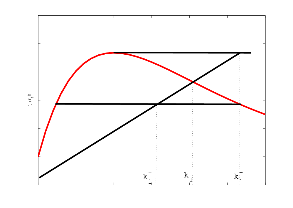
In a similar manner, one can find (5.32) has two equilibrium (0,0)(0,0) and (k1+,k2+)(k_{1}^{+},k_{2}^{+}) satisfying

α+δ​k1+=r1+r1​h+​(k1+)k2+=h+​(k1+).\begin{split}\alpha+\delta k_{1}^{+}&=r_{1}+r_{1}h^{+}(k_{1}^{+})\\ k_{2}^{+}&=h^{+}(k_{1}^{+}).\end{split} (5.33)

Since h+≥hh^{+}\geq h, from the first equation of (5.31), it is easily seen that that k1+≥k1k_{1}^{+}\geq k_{1}. In addition, since k1>hm,k_{1}>h_{m}, we have k2+=h+​(k1+)=h⁡(hm)≥h⁡(k1)=k2.k_{2}^{+}=h^{+}(k_{1}^{+})=h(h_{m})\geq h(k_{1})=k_{2}.

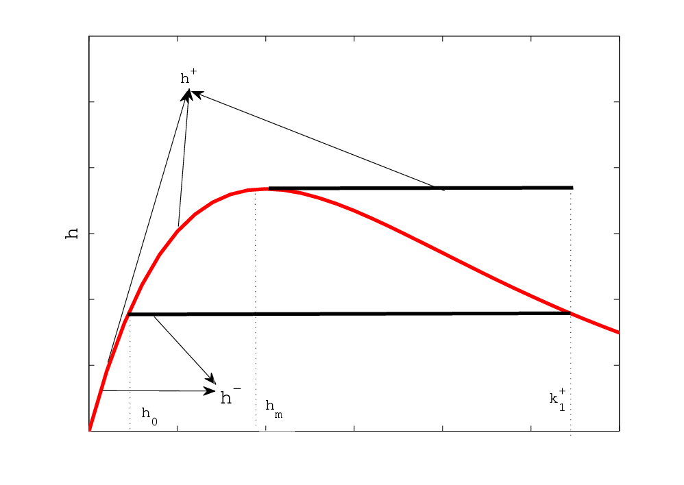
Now there is a h0∈(0,hm]h_{0}\in(0,h_{m}] such that h⁡(h0)=h⁡(k1+)h(h_{0})=h(k_{1}^{+}) and define

h−​(w1)={h⁡(w1),   0≤w1≤h0,h⁡(k1+),w1>h0.h^{-}(w_{1})=\left\{\begin{array}[]{ll}h(w_{1}),&\;\;\;0\leq w_{1}\leq h_{0},\\[5.69046pt] h(k_{1}^{+}),&\;\;\;w_{1}>h_{0}.\end{array}\right.

Then

0<h−​(w1)≤h⁡(w1)≤h+​(w1)≤h′​(0)​w1,w1∈(0,k1+]0<h^{-}(w_{1})\leq h(w_{1})\leq h^{+}(w_{1})\leq h^{\prime}(0)w_{1},w_{1}\in(0,k^{+}_{1}]
Refer to caption
Figure 3: The construction of h+h^{+} and h−h^{-}. The red curve is hh.
Refer to caption
Figure 4: The intersections of r1+r1​h​(w1),r1+r1​h±​(w1)r_{1}+r_{1}h(w_{1}),r_{1}+r_{1}h^{\pm}(w_{1}) with the line α+δ​w1\alpha+\delta w_{1}. The red curve is r1+r1​hr_{1}+r_{1}h

The corresponding cooperative system for h−h^{-} is

∂w1∂t=d1​Δ​w1+w1​[r1−α−δ​w1+r1​w2]∂w2∂t=d2​Δ​w2+r2​(1+w2)​[−w2+h−​(w1)]\begin{split}\frac{\partial w_{1}}{\partial t}&=d_{1}\Delta w_{1}+w_{1}[r_{1}-\alpha-\delta w_{1}+r_{1}w_{2}]\\ \frac{\partial w_{2}}{\partial t}&=d_{2}\Delta w_{2}+r_{2}(1+w_{2})[-w_{2}+h^{-}(w_{1})]\\ \end{split} (5.34)

In a similar manner, one can find (5.34) has two equilibrium (0,0)(0,0) and (k1−,k2−)(k_{1}^{-},k_{2}^{-}) satisfying

α+δ​k1−=r1+r1​h−​(k1−)k2−=h−​(k1−).\begin{split}\alpha+\delta k_{1}^{-}&=r_{1}+r_{1}h^{-}(k_{1}^{-})\\ k_{2}^{-}&=h^{-}(k_{1}^{-}).\end{split} (5.35)

Similarly, we have k1−≤k1.k_{1}^{-}\leq k_{1}. In addition, by the definition of h−h^{-}, we have

k2−=h−​(k1−)≤h⁡(k1+)≤h⁡(k1)=k2.k_{2}^{-}=h^{-}(k_{1}^{-})\leq h(k^{+}_{1})\leq h(k_{1})=k_{2}.

Thus,

(0,0)<<(k1−,k2−)≤(k1,k2)≤(k1+,k2+).(0,0)<<(k_{1}^{-},k_{2}^{-})\leq(k_{1},k_{2})\leq(k_{1}^{+},k_{2}^{+}).

See Remark 2.3 for (H1)(i). Now it is straightforward to check all other conditions of (H1)(i)-(iv).

The spreading results for the cooperative systems were used to establish in [36]. We now demonstrate Theorem 2.1 can be used to establish spreading speed and traveling wave solutions of the nonmonotone system (5.26) and summarize the results in the following theorem.

Theorem 5.1

Let d1,α,δ,r1,d2,r2d_{1},\alpha,\delta,r_{1},d_{2},r_{2} be all positive numbers. Assume d1≥d2d_{1}\geq d_{2}, α<r1\alpha<r_{1}, k1>hmk_{1}>h_{m} and

δ≥r1​r2​h′​(0)r1+r2−α.\begin{split}\delta&\geq\frac{r_{1}r_{2}h^{\prime}(0)}{r_{1}+r_{2}-\alpha}.\end{split} (5.36)

Then the conclusions of Theorem 2.1 hold for (5.26) for the minimum speed c∗=2​(r1−α)​d1c^{*}=2\sqrt{(r_{1}-\alpha)d_{1}}, Λc=c−c2−4​d1​(r1−α)2​d1>0\Lambda_{c}=\frac{c-\sqrt{c^{2}-4d_{1}(r_{1}-\alpha)}}{2d_{1}}>0 and νΛc\nu_{\Lambda_{c}}, where νλ\nu_{\lambda} is defined in (5.39).

We now need to check (H2) and (H3). The linearization of (5.26) at the origin is

∂w1∂t=d1​Δ​w1+(r1−α)​w1∂w2∂t=d2​Δ​w2+r2​(h′​(0)​w1−w2)\begin{split}\frac{\partial w_{1}}{\partial t}&=d_{1}\Delta w_{1}+(r_{1}-\alpha)w_{1}\\ \frac{\partial w_{2}}{\partial t}&=d_{2}\Delta w_{2}+r_{2}(h^{\prime}(0)w_{1}-w_{2})\\ \end{split} (5.37)

The matrix in (1.8) for (5.26) is

Aλ=(aλi,j)=(d1​λ2+r1−α   0r2​h′​(0)d2​λ2−r2)\begin{split}A_{\lambda}=(a^{i,j}_{\lambda})=\left(\begin{array}[]{ll}d_{1}\lambda^{2}+r_{1}-\alpha&\;\;\;0\\ r_{2}h^{\prime}(0)&d_{2}\lambda^{2}-r_{2}\\ \end{array}\right)\end{split} (5.38)

It is easy to see that (H2) holds. In fact, the principle eigenvalue AλA_{\lambda} is Ψ⁡(Aλ)=d1​λ2+r1−α\Psi(A_{\lambda})=d_{1}\lambda^{2}+r_{1}-\alpha, which is a convex function of λ\lambda. And

Φ⁡(λ)=Ψ⁡(Aλ)λ=d1​λ2+r1−αλ\Phi(\lambda)=\frac{\Psi(A_{\lambda})}{\lambda}=\frac{d_{1}\lambda^{2}+r_{1}-\alpha}{\lambda}

satisfies the results of Lemma 1.1. In fact Φ⁡(λ)\Phi(\lambda) is also a strictly convex function of λ\lambda. The minimum of Φ⁡(λ)\Phi(\lambda) is c∗=2​(r1−α)​d1c^{*}=2\sqrt{(r_{1}-\alpha)d_{1}}. For each λ>0\lambda>0, the positive eigenvector of AλA_{\lambda} corresponding to Ψ⁡(λ)\Psi(\lambda) is

νλ=(νλ1νλ2)=((d1−d2)​λ2+r1+r2−αr2​h′​(0))\nu_{\lambda}=\left(\begin{array}[]{c}\nu_{\lambda}^{1}\\ \nu_{\lambda}^{2}\\ \end{array}\right)=\left(\begin{array}[]{c}(d_{1}-d_{2})\lambda^{2}+r_{1}+r_{2}-\alpha\\ r_{2}h^{\prime}(0)\end{array}\right) (5.39)

which is also the positive eigenvector of 1λ​Aλ\frac{1}{\lambda}A_{\lambda} corresponding to Φ⁡(λ)\Phi(\lambda).

For each c>c∗c>c^{*}, the left positive solution of Φ⁡(λ)=c\Phi(\lambda)=c is

Λc=c−c2−4​d1​(r1−α)2​d1\Lambda_{c}=\frac{c-\sqrt{c^{2}-4d_{1}(r_{1}-\alpha)}}{2d_{1}}

in Lemma 1.1. Further from (5.39) we can see that

νλ2νλ1=r2​h′​(0)(d1−d2)​λ2+r1+r2−α=h′​(0)σ\frac{\nu_{\lambda}^{2}}{\nu_{\lambda}^{1}}=\frac{r_{2}h^{\prime}(0)}{(d_{1}-d_{2})\lambda^{2}+r_{1}+r_{2}-\alpha}=\frac{h^{\prime}(0)}{\sigma}

where σ=1+r1−α+(d1−d2)​λ2r2>1.\sigma=1+\frac{r_{1}-\alpha+(d_{1}-d_{2})\lambda^{2}}{r_{2}}>1.

In order to verify (H3) for (5.32) let

(w1,w2)=(θ,θ​h′​(0)σ)>>(0,0),θ>0.(w_{1},w_{2})=(\theta,\theta\frac{h^{\prime}(0)}{\sigma})>>(0,0),\;\theta>0.

Thus (H3) is equivalent to the following two inequalities

w1​[r1−α−δ​w1+r1​w2]≤(r1−α)​w1r2​(1+w2)​[−w2+h+​(w1)]≤r2​(h′​(0)​w1−w2)\begin{split}w_{1}[r_{1}-\alpha-\delta w_{1}+r_{1}w_{2}]&\leq(r_{1}-\alpha)w_{1}\\ r_{2}(1+w_{2})[-w_{2}+h^{+}(w_{1})]&\leq r_{2}(h^{\prime}(0)w_{1}-w_{2})\\ \end{split}

or

δ​w1≥r1​w2\begin{split}\delta w_{1}&\geq r_{1}w_{2}\\ \end{split} (5.40)

and

h′​(0)​w1+w22≥h+​(w1)​(1+w2)\begin{split}h^{\prime}(0)w_{1}+w^{2}_{2}&\geq h^{+}(w_{1})(1+w_{2})\\ \end{split} (5.41)

It follows that the following equality suffices to verify (5.40):

δ​θ≥r1​θ​h′​(0)1+r1−αr2,\delta\theta\geq r_{1}\theta\frac{h^{\prime}(0)}{1+\frac{r_{1}-\alpha}{r_{2}}},

which is true if (5.36) holds.

In order to verify (5.41), following Weinberger, Kawasaki and Shigesada [36], there always is a positive constant ς\varsigma such that

w2=h′​(0)ς​w1.w_{2}=\frac{h^{\prime}(0)}{\varsigma}w_{1}.

Substituting w2w_{2} into (5.41) and multiplying ς2h′​(0)​w1\frac{\varsigma^{2}}{h^{\prime}(0)w_{1}} at the both sides, we get

ς2+h′​(0)​w1≥ς2​h+​(w1)h′​(0)​w1+ς​h+​(w1).\varsigma^{2}+h^{\prime}(0)w_{1}\geq\frac{\varsigma^{2}h^{+}(w_{1})}{h^{\prime}(0)w_{1}}+\varsigma h^{+}(w_{1}).

Rearranging the terms produces

−ς2(1−h+​(w1)h′​(0)​w1)+ςh+(w1)−h′(0)w1≤0,w1>0.\begin{split}-\varsigma^{2}\big(1-\frac{h^{+}(w_{1})}{h^{\prime}(0)w_{1}}\big)+\varsigma h^{+}(w_{1})-h^{\prime}(0)w_{1}\leq 0,\;\;w_{1}>0.\end{split} (5.42)

Recall the definition that h+​(w1)=h⁡(w1)h^{+}(w_{1})=h(w_{1}) for w1≤hmw_{1}\leq h_{m} and h+​(w1)=h⁡(hm)h^{+}(w_{1})=h(h_{m}) for w1>hmw_{1}>h_{m}. Since the left side of (5.42) is decreasing in w1w_{1} for w1>hmw_{1}>h_{m}, we only need to verify (5.42) for w1≤hmw_{1}\leq h_{m}.

By the quadratic formula, the discriminant of (5.42) for w1≤hmw_{1}\leq h_{m} is

h​(w1)2−4​(1−h⁡(w1)h′​(0)​w1)​h′​(0)​w1=h​(w1)2+4​h​(w1)−4​h′​(0)​w1,h(w_{1})^{2}-4\big(1-\frac{h(w_{1})}{h^{\prime}(0)w_{1}}\big)h^{\prime}(0)w_{1}=h(w_{1})^{2}+4h(w_{1})-4h^{\prime}(0)w_{1},

which is negative from (5.27). Thus the left side of (5.42) has no real zeros and it has to be nonpositive because of the assumption that 1−h+​(w1)h′​(0)​w1>01-\frac{h^{+}(w_{1})}{h^{\prime}(0)w_{1}}>0 for w1>0w_{1}>0. In fact, (5.27) is is one of the three possible conditions in [36] to guarantee (5.42) holds.

Notice that h±h^{\pm} and hh are identical around the origin. By the exact same arguments (just replacing ki+k_{i}^{+} by ki−k^{-}_{i} and h+h^{+} by h−h^{-}), we can verify that (H3) holds for (5.34) as well.

6 Appendix

In this section, we shall verify provide a direct verification of Lemmas 4.3 and 4.4. Lower and upper solutions of the equivalent integral equations (4.15) play a central role in the construction of fixed points of the equivalent integral equations through monotone iterations. The lower and upper solutions give asymptotic behavior of traveling wave solutions of (1.3).

Wu and Zou [38, 39], Ma [22, 23] verify lower and upper solutions through differential equations, and then use them in monotone iterations of equivalent integral equations. While it was pointed out in [3] that the upper and lower solutions for differential equations are required to be smooth for delayed equations, the author [29] recently directly verified ϕ+\phi^{+} and ϕ−\phi^{-} are indeed lower and upper solutions through the equivalent integral equations for scalar equations, where the integrals and compare the two sides of (4.15) were calculated and compared. Clearly, in this way, the lower and upper solutions are not required to be smooth.

In this appendix, we shall directly verify that, for nn-dimensional systems, ϕ+\phi^{+} and ϕ−\phi^{-} are the lower and upper solutions of (4.15). Thus this Appendix can be viewed as a continuation of [29] for the direct verification of non-smooth upper and lower solutions of the equivalent integral equations for nn-dimensional systems.

It should be pointed out that the proof of two lemmas in Ma [22, Lemmas 2.5, 2.6] can significantly simplify the verification of lower and upper solutions for the equivalent integral equations although the conclusions of the two lemmas in [22] were about lower and upper solutions for differential equations (see [31, Section 6.1] for more details). As a result, we always can verify them in a much simpler way. Nevertheless, a direct verification can provide a further evidence that ϕ+\phi^{+} and ϕ−\phi^{-} are lower and upper solutions. In addition, by carefully analyzing eigenvalues and corresponding eigenvectors, we identify some identities between the parameters and reveal interesting relations between the parameters.

The results in this appendix are natural extensions of those in the author [29] for scalar cases. As in [29], for λ>0\lambda>0 let

(Mi​(λ))=β​νλ−λ2​D​νλ+Aλ​νλ(M_{i}(\lambda))=\beta\nu_{\lambda}-\lambda^{2}D\nu_{\lambda}+A_{\lambda}\nu_{\lambda}

or

Mi(λ)=βνλi−νλidiλ2+∑j=1Nνλjaλi​j,i=1,…,N,M_{i}(\lambda)=\beta\nu^{i}_{\lambda}-\nu^{i}_{\lambda}d_{i}\lambda^{2}+\sum_{j=1}^{N}\nu^{j}_{\lambda}a^{ij}_{\lambda},i=1,...,N, (6.43)

where νλ=(νλi)\nu_{\lambda}=(\nu^{i}_{\lambda}) is the positive eigenvector of 1λ​Aλ\frac{1}{\lambda}A_{\lambda} in (1.8) corresponding to the principle eigenvalue Φ⁡(λ)\Phi(\lambda). For c>c∗c>c^{*}, recall that Φ⁡(Λc)=c\Phi(\Lambda_{c})=c. It follows that 1Λc​AΛc​νΛc=Φ⁡(Λc)​νΛc=c​νΛc\frac{1}{\Lambda_{c}}A_{\Lambda_{c}}\nu_{\Lambda_{c}}=\Phi(\Lambda_{c})\nu_{\Lambda_{c}}=c\nu_{\Lambda_{c}} and

Mi(Λc)=(β−diΛc2+cΛc)νΛci,i=1,…,N.M_{i}(\Lambda_{c})=(\beta-d_{i}\Lambda_{c}^{2}+c\Lambda_{c})\nu^{i}_{\Lambda_{c}},i=1,...,N.

Because of (4.12), Mi(Λc)>0,i=1,…,N.M_{i}(\Lambda_{c})>0,i=1,...,N. Noting Mi​(λ)M_{i}(\lambda) is continuous with respect to λ\lambda, we always can choose a γ\gamma such that

1<γ<2,Mi(γΛc)>0,i=1,…,N.1<\gamma<2,\;\;M_{i}(\gamma\Lambda_{c})>0,i=1,...,N. (6.44)

In order to simply our proofs, we first prove two identities (Lemmas 6.1, 6.2), which are the extension of the identities for scalar cases in [29]. Their proofs are almost identical to those in [29] except that eigenvector νλi\nu^{i}_{\lambda} has to be included.

Lemma 6.1

Assume (H​1−H​2)(H1-H2) hold. Then for each c>c∗c>c^{*}

Mi​(Λc)di​(λ1​i+λ2​i)(1λ1​i+Λc+1λ2​i−Λc)=νΛci,i=1,…,N.\frac{M_{i}(\Lambda_{c})}{d_{i}(\lambda_{1i}+\lambda_{2i})}\Big(\frac{1}{\lambda_{1i}+\Lambda_{c}}+\frac{1}{\lambda_{2i}-\Lambda_{c}}\Big)=\nu^{i}_{\Lambda_{c}},i=1,...,N. (6.45)
{@proof}

[Proof.]Recall λ2​i>λ1​i>2​Λc>Λc\lambda_{2i}>\lambda_{1i}>2\Lambda_{c}>\Lambda_{c}. It follows that, i=1,…,Ni=1,...,N,

Mi​(Λc)di​(λ1​i+λ2​i)​(1λ1​i+Λc+1λ2​i−Λc)=Mi​(Λc)di​(λ1​i+λ2​i)​(λ1​i+λ2​i)λ1​i​λ2​i+(λ2​i−λ1​i)​Λc−Λc2=Mi​(Λc)di​1βdi+cdi​Λc−Λc2=Mi​(Λc)​1β+c​Λc−di​Λc2=β​νΛci+νΛci​(c​Λc−di​Λc2)β+c​Λc−di​Λc2=νΛci.\begin{split}&\frac{M_{i}(\Lambda_{c})}{d_{i}(\lambda_{1i}+\lambda_{2i})}\Big(\frac{1}{\lambda_{1i}+\Lambda_{c}}+\frac{1}{\lambda_{2i}-\Lambda_{c}}\Big)\\ &=\frac{M_{i}(\Lambda_{c})}{d_{i}(\lambda_{1i}+\lambda_{2i})}\frac{(\lambda_{1i}+\lambda_{2i})}{\lambda_{1i}\lambda_{2i}+(\lambda_{2i}-\lambda_{1i})\Lambda_{c}-\Lambda_{c}^{2}}\\ &=\frac{M_{i}(\Lambda_{c})}{d_{i}}\frac{1}{\frac{\beta}{d_{i}}+\frac{c}{d_{i}}\Lambda_{c}-\Lambda_{c}^{2}}\\ &=M_{i}(\Lambda_{c})\frac{1}{\beta+c\Lambda_{c}-d_{i}\Lambda_{c}^{2}}\\ &=\frac{\beta\nu^{i}_{\Lambda_{c}}+\nu^{i}_{\Lambda_{c}}(c\Lambda_{c}-d_{i}\Lambda_{c}^{2})}{\beta+c\Lambda_{c}-d_{i}\Lambda_{c}^{2}}\\ &=\nu^{i}_{\Lambda_{c}}.\end{split} (6.46)

□\quad\Box

Lemma 6.2

Assume (H​1−H​2)(H1-H2) hold and γ\gamma satisfies (6.44). Then for each c>c∗c>c^{*}, i=1,…,Ni=1,...,N

Mi​(Λc)(λ1​i+Λc)​νΛci+Mi​(Λc)(λ2​i−Λc)​νΛci−Mi​(γ​Λc)(λ1​i+γ​Λc)​νγ​Λci−Mi​(γ​Λc)(λ2​i−γ​Λc)​νγ​Λci>0.\frac{M_{i}(\Lambda_{c})}{(\lambda_{1i}+\Lambda_{c})\nu^{i}_{\Lambda_{c}}}+\frac{M_{i}(\Lambda_{c})}{(\lambda_{2i}-\Lambda_{c})\nu^{i}_{\Lambda_{c}}}-\frac{M_{i}(\gamma\Lambda_{c})}{(\lambda_{1i}+\gamma\Lambda_{c})\nu^{i}_{\gamma\Lambda_{c}}}-\frac{M_{i}(\gamma\Lambda_{c})}{(\lambda_{2i}-\gamma\Lambda_{c})\nu^{i}_{\gamma\Lambda_{c}}}>0. (6.47)
{@proof}

[Proof.]Since λ2​i>λ1​i>2​Λc\lambda_{2i}>\lambda_{1i}>2\Lambda_{c}, it follows that λ2​i>γ​Λc>Λc.\lambda_{2i}>\gamma\Lambda_{c}>\Lambda_{c}. Lemma 1.1 (Φ⁡(γ​Λc)<c\Phi(\gamma\Lambda_{c})<c) implies that, for i=1,…,Ni=1,...,N

Mi​(γ​Λc)=β​νγ​Λci−νγ​Λci​di​(γ​Λc)2+∑j=1,…,Nνγ​Λcj​aγ​Λci​j=(β−di​(γ​Λc)2+Φ⁡(γ​Λc)​γ​Λc)​νγ​Λci<(β−di​(γ​Λc)2+c​γ​Λc)​νγ​Λci.\begin{split}M_{i}(\gamma\Lambda_{c})&=\beta\nu^{i}_{\gamma\Lambda_{c}}-\nu^{i}_{\gamma\Lambda_{c}}d_{i}(\gamma\Lambda_{c})^{2}+\sum_{j=1,...,N}\nu^{j}_{\gamma\Lambda_{c}}a^{ij}_{\gamma\Lambda_{c}}\\ &=\big(\beta-d_{i}(\gamma\Lambda_{c})^{2}+\Phi(\gamma\Lambda_{c})\gamma\Lambda_{c}\big)\nu^{i}_{\gamma\Lambda_{c}}\\ &<(\beta-d_{i}(\gamma\Lambda_{c})^{2}+c\gamma\Lambda_{c})\nu^{i}_{\gamma\Lambda_{c}}.\end{split} (6.48)

We also note Mi​(Λc)=(β+c​Λc−di​Λc2)​νΛciM_{i}(\Lambda_{c})=(\beta+c\Lambda_{c}-d_{i}\Lambda_{c}^{2})\nu^{i}_{\Lambda_{c}}. Thus, for i=1,…,Ni=1,...,N, we have

Mi​(Λc)(λ1​i+Λc)​νΛci+Mi​(Λc)(λ2​i−Λc)​νΛci−Mi​(γ​Λc)(λ1​i+γ​Λc)​νγ​Λci−Mi​(γ​Λc)(λ2​i−γ​Λc)​νγ​Λci=(λ1​i+λ2​i)​Mi​(Λc)(λ1​i​λ2​i+(λ2​i−λ1​i)​Λc−Λc2)​νΛci−(λ1​i+λ2​i)​Mi​(γ​Λc)(λ1​i​λ2​i+(λ2​i−λ1​i)​γ​Λc−(γ​Λc)2)​νγ​Λci=c2+4​β​didi​Mi​(Λc)(βdi+cdi​Λc−Λc2)​νΛci−c2+4​β​didi​Mi​(γ​Λc)(βdi+cdi​γ​Λc−(γ​Λc)2)​νγ​Λci=c2+4​β​di​Mi​(Λc)(β+c​Λc−di​Λc2)​νΛci−c2+4​β​di​Mi​(γ​Λc)(β+c​γ​Λc−di​(γ​Λc)2)​νγ​Λci=c2+4​β​di​(Mi​(Λc)(β+c​Λc−di​Λc2)​νΛci−Mi​(γ​Λc)(β+c​γ​Λc−di​(γ​Λc)2)​νγ​Λci)=c2+4​β​di​(1−Mi​(γ​Λc)(β+c​γ​Λc−di​(γ​Λc)2)​νγ​Λci)>0.\begin{split}&\frac{M_{i}(\Lambda_{c})}{(\lambda_{1i}+\Lambda_{c})\nu^{i}_{\Lambda_{c}}}+\frac{M_{i}(\Lambda_{c})}{(\lambda_{2i}-\Lambda_{c})\nu^{i}_{\Lambda_{c}}}-\frac{M_{i}(\gamma\Lambda_{c})}{(\lambda_{1i}+\gamma\Lambda_{c})\nu^{i}_{\gamma\Lambda_{c}}}-\frac{M_{i}(\gamma\Lambda_{c})}{(\lambda_{2i}-\gamma\Lambda_{c})\nu^{i}_{\gamma\Lambda_{c}}}\\ &=\frac{(\lambda_{1i}+\lambda_{2i})M_{i}(\Lambda_{c})}{(\lambda_{1i}\lambda_{2i}+(\lambda_{2i}-\lambda_{1i})\Lambda_{c}-\Lambda_{c}^{2})\nu^{i}_{\Lambda_{c}}}-\frac{(\lambda_{1i}+\lambda_{2i})M_{i}(\gamma\Lambda_{c})}{(\lambda_{1i}\lambda_{2i}+(\lambda_{2i}-\lambda_{1i})\gamma\Lambda_{c}-(\gamma\Lambda_{c})^{2})\nu^{i}_{\gamma\Lambda_{c}}}\\ &=\frac{\frac{\sqrt{c^{2}+4\beta d_{i}}}{d_{i}}M_{i}(\Lambda_{c})}{(\frac{\beta}{d_{i}}+\frac{c}{d_{i}}\Lambda_{c}-\Lambda_{c}^{2})\nu^{i}_{\Lambda_{c}}}-\frac{\frac{\sqrt{c^{2}+4\beta d_{i}}}{d_{i}}M_{i}(\gamma\Lambda_{c})}{(\frac{\beta}{d_{i}}+\frac{c}{d_{i}}\gamma\Lambda_{c}-(\gamma\Lambda_{c})^{2})\nu^{i}_{\gamma\Lambda_{c}}}\\ &=\frac{\sqrt{c^{2}+4\beta d_{i}}M_{i}(\Lambda_{c})}{(\beta+c\Lambda_{c}-d_{i}\Lambda_{c}^{2})\nu^{i}_{\Lambda_{c}}}-\frac{\sqrt{c^{2}+4\beta d_{i}}M_{i}(\gamma\Lambda_{c})}{(\beta+c\gamma\Lambda_{c}-d_{i}(\gamma\Lambda_{c})^{2})\nu^{i}_{\gamma\Lambda_{c}}}\\ &=\sqrt{c^{2}+4\beta d_{i}}\big(\frac{M_{i}(\Lambda_{c})}{(\beta+c\Lambda_{c}-d_{i}\Lambda_{c}^{2})\nu^{i}_{\Lambda_{c}}}-\frac{M_{i}(\gamma\Lambda_{c})}{(\beta+c\gamma\Lambda_{c}-d_{i}(\gamma\Lambda_{c})^{2})\nu^{i}_{\gamma\Lambda_{c}}}\big)\\ &=\sqrt{c^{2}+4\beta d_{i}}\big(1-\frac{M_{i}(\gamma\Lambda_{c})}{(\beta+c\gamma\Lambda_{c}-d_{i}(\gamma\Lambda_{c})^{2})\nu^{i}_{\gamma\Lambda_{c}}}\big)\\ &>0.\end{split} (6.49)

This completes the proof. □\quad\Box

6.1 Proof of Lemma 4.3

The proof of Lemma 4.3 is almost identical to that in [29] for the scalar case except that the eigenvector νλi\nu^{i}_{\lambda} needs to be included, and delay terms are not present here. {@proof}[Proof.]Let ξ∗i=ln⁡kiνΛciΛc,i=1,…,N.\xi^{*}_{i}=\frac{\ln\frac{k_{i}}{\nu^{i}_{\Lambda_{c}}}}{\Lambda_{c}},i=1,...,N. Then ϕi+​(ξ)=ki\phi^{+}_{i}(\xi)=k_{i} if ξ≥ξi∗\xi\geq\xi^{*}_{i}, and ϕi+​(ξ)=νΛci​eΛc​ξ\phi^{+}_{i}(\xi)=\nu^{i}_{\Lambda_{c}}e^{\Lambda_{c}\xi} if ξ<ξ∗i,i=1,…,N.\xi<\xi^{*}_{i},i=1,...,N. Note that ϕi+​(ξ)≤νΛci​eΛc​ξ,ξ∈ℝ.\phi^{+}_{i}(\xi)\leq\nu^{i}_{\Lambda_{c}}e^{\Lambda_{c}\xi},\xi\in\mathbb{R}. In view of (H1)-(H3) we have, for ξ≤ξi∗\xi\leq\xi^{*}_{i}

Hi​(ϕ+​(ξ))=β​ϕi+​(ξ)+fi​(ϕ+​(ξ))≤β​ϕi+​(ξ)+∑j=1n∂jfi​(0)​ϕj+​(ξ)≤Mi​(Λc)​eΛc​ξ,\begin{split}H_{i}(\phi^{+}(\xi))&=\beta\phi_{i}^{+}(\xi)+f_{i}(\phi^{+}(\xi))\\ &\leq\beta\phi_{i}^{+}(\xi)+\sum_{j=1}^{n}\partial_{j}f_{i}(0)\phi_{j}^{+}(\xi)\\ &\leq M_{i}(\Lambda_{c})e^{\Lambda_{c}\xi},\end{split}

where Mi(.)M_{i}(.) is defined in (6.43). For ξ≥ξi∗\xi\geq\xi^{*}_{i}, because of the assumption that (1.3) is cooperative and β\beta is sufficiently large, we have

Hi​(ϕ+​(ξ))≤β​ki+fi​(k)=β​ki.\begin{split}H_{i}(\phi^{+}(\xi))&\leq\beta k_{i}+f_{i}(k)\\ &=\beta k_{i}.\end{split}

Thus, for ξ≥ξ∗i,i=1,…,N\xi\geq\xi^{*}_{i},i=1,...,N, we obtain

𝒯i​[ϕ+]​(ξ)≤Mi​(Λc)di​(λ1​i+λ2​i)​∫−∞ξi∗e−λ1​i​(ξ−s)​eΛc​s​𝑑s+1di​(λ1​i+λ2​i)​[∫ξi∗ξe−λ1​i​(ξ−s)​β​ki​ds+∫ξ∞eλ2​i​(ξ−s)​β​ki​ds].\begin{split}\mathcal{T}_{i}[\phi^{+}](\xi)&\leq\frac{M_{i}(\Lambda_{c})}{d_{i}(\lambda_{1i}+\lambda_{2i})}\int_{-\infty}^{\xi^{*}_{i}}e^{-\lambda_{1i}(\xi-s)}e^{\Lambda_{c}s}ds\\ &\quad+\frac{1}{d_{i}(\lambda_{1i}+\lambda_{2i})}[\int_{\xi^{*}_{i}}^{\xi}e^{-\lambda_{1i}(\xi-s)}\beta k_{i}ds+\int^{\infty}_{\xi}e^{\lambda_{2i}(\xi-s)}\beta k_{i}ds].\\ \end{split} (6.50)

Thus in view of (4.14), we add and subtract the term β​kidi​(λ1​i+λ2​i)​∫−∞ξi∗e−λ1​i​(ξ−s)​𝑑s\frac{\beta k_{i}}{d_{i}(\lambda_{1i}+\lambda_{2i})}\int_{-\infty}^{\xi^{*}_{i}}e^{-\lambda_{1i}(\xi-s)}ds at the left of (6.50). Now for i=1,…,N,ξ≥ξi∗i=1,...,N,\xi\geq\xi^{*}_{i}, noting that νΛci​eΛc​ξi∗=ki\nu^{i}_{\Lambda_{c}}e^{\Lambda_{c}\xi^{*}_{i}}=k_{i}, (6.50) can be written as

𝒯i​[ϕ+]​(ξ)≤ki+1di​(λ1​i+λ2​i)​(Mi​(Λc)​∫−∞ξi∗e−λ1​i​(ξ−s)​eΛc​s​𝑑sCLOSE−βki∫−∞ξi∗e−λ1​i​(ξ−s)ds)=ki+1di​(λ1​i+λ2​i)​(Mi​(Λc)​e−λ1​i​ξ​e(λ1​i+Λc)​ξi∗λ1​i+Λc−β​ki​e−λ1​i​ξ​eλ1​i​ξi∗λ1​i)=ki+ki​e−λ1​i​ξ​eλ1​i​ξi∗di​(λ1​i+λ2​i)​(Mi​(Λc)(λ1​i+Λc)​νΛci−βλ1​i)=ki+ki​e−λ1​i​ξ​eλ1​i​ξi∗di​(λ1​i+λ2​i)​(λ1​i+Λc)​λ1​i​νΛci​(λ1​i​(Mi​(Λc)−νΛci​β)−νΛci​β​Λc).\begin{split}\mathcal{T}_{i}[\phi^{+}](\xi)&\leq k_{i}+\frac{1}{d_{i}(\lambda_{1i}+\lambda_{2i})}\big(M_{i}(\Lambda_{c})\int_{-\infty}^{\xi^{*}_{i}}e^{-\lambda_{1i}(\xi-s)}e^{\Lambda_{c}s}ds\\ &\quad-\beta k_{i}\int_{-\infty}^{\xi^{*}_{i}}e^{-\lambda_{1i}(\xi-s)}ds\big)\\ &=k_{i}+\frac{1}{d_{i}(\lambda_{1i}+\lambda_{2i})}\big(M_{i}(\Lambda_{c})\frac{e^{-\lambda_{1i}\xi}e^{(\lambda_{1i}+\Lambda_{c})\xi^{*}_{i}}}{\lambda_{1i}+\Lambda_{c}}-\beta k_{i}\frac{e^{-\lambda_{1i}\xi}e^{\lambda_{1i}\xi^{*}_{i}}}{\lambda_{1i}}\big)\\ &=k_{i}+\frac{k_{i}e^{-\lambda_{1i}\xi}e^{\lambda_{1i}\xi^{*}_{i}}}{d_{i}(\lambda_{1i}+\lambda_{2i})}\big(\frac{M_{i}(\Lambda_{c})}{(\lambda_{1i}+\Lambda_{c})\nu^{i}_{\Lambda_{c}}}-\frac{\beta}{\lambda_{1i}}\big)\\ &=k_{i}+\frac{k_{i}e^{-\lambda_{1i}\xi}e^{\lambda_{1i}\xi^{*}_{i}}}{d_{i}(\lambda_{1i}+\lambda_{2i})(\lambda_{1i}+\Lambda_{c})\lambda_{1i}\nu^{i}_{\Lambda_{c}}}\big(\lambda_{1i}(M_{i}(\Lambda_{c})-\nu^{i}_{\Lambda_{c}}\beta)-\nu^{i}_{\Lambda_{c}}\beta\Lambda_{c}\big).\end{split} (6.51)

Since Mi(Λc)=βνΛci−νΛcidiΛc2+cΛcνΛci,i=1,…,NM_{i}(\Lambda_{c})=\beta\nu^{i}_{\Lambda_{c}}-\nu^{i}_{\Lambda_{c}}d_{i}\Lambda_{c}^{2}+c\Lambda_{c}\nu^{i}_{\Lambda_{c}},i=1,...,N, we have, i=1,…,Ni=1,...,N

λ1​i​(Mi​(Λc)−νΛci​β)−β​νΛci​Λc=νΛci​λ1​i​(c​Λc−di​Λc2)−β​νΛci​Λc=νΛci​4​β​di2​di​(c2+4​β​di+c)​(c​Λc−di​Λc2)−β​νΛci​Λc=νΛci​4​β​(c​Λc−di​Λc2)−2​(c2+4​β​di+c)​β​Λc2​(c2+4​β​di+c)=νΛci​2​β​Λc​(2​c−2​di​Λc−c2+4​β​di−c)2​(c2+4​β​di+c)=νΛci​2​β​Λc​(c−2​di​Λc−c2+4​β​di)2​(c2+4​β​di+c)<0.\begin{split}&\lambda_{1i}(M_{i}(\Lambda_{c})-\nu^{i}_{\Lambda_{c}}\beta)-\beta\nu^{i}_{\Lambda_{c}}\Lambda_{c}\\ &=\nu^{i}_{\Lambda_{c}}\lambda_{1i}(c\Lambda_{c}-d_{i}\Lambda_{c}^{2})-\beta\nu^{i}_{\Lambda_{c}}\Lambda_{c}\\ &=\nu^{i}_{\Lambda_{c}}\frac{4\beta d_{i}}{2d_{i}(\sqrt{c^{2}+4\beta d_{i}}+c)}(c\Lambda_{c}-d_{i}\Lambda_{c}^{2})-\beta\nu^{i}_{\Lambda_{c}}\Lambda_{c}\\ &=\nu^{i}_{\Lambda_{c}}\frac{4\beta(c\Lambda_{c}-d_{i}\Lambda_{c}^{2})-2(\sqrt{c^{2}+4\beta d_{i}}+c)\beta\Lambda_{c}}{2(\sqrt{c^{2}+4\beta d_{i}}+c)}\\ &=\nu^{i}_{\Lambda_{c}}\frac{2\beta\Lambda_{c}\big(2c-2d_{i}\Lambda_{c}-\sqrt{c^{2}+4\beta d_{i}}-c\big)}{2(\sqrt{c^{2}+4\beta d_{i}}+c)}\\ &=\nu^{i}_{\Lambda_{c}}\frac{2\beta\Lambda_{c}\big(c-2d_{i}\Lambda_{c}-\sqrt{c^{2}+4\beta d_{i}}\big)}{2(\sqrt{c^{2}+4\beta d_{i}}+c)}\\ &<0.\\ \end{split} (6.52)

Combining (6.51) and (6.52), we see that for ξ≥ξ∗i,i=1,…,N\xi\geq\xi^{*}_{i},i=1,...,N,

𝒯i​[ϕ+]​(ξ)≤ki.\mathcal{T}_{i}[\phi^{+}](\xi)\leq k_{i}. (6.53)

Similarly, noting νΛci​eΛc​ξi∗=ki\nu^{i}_{\Lambda_{c}}e^{\Lambda_{c}\xi^{*}_{i}}=k_{i}, one can see that, for ξ≤ξ∗i,i=1,…,N\xi\leq\xi^{*}_{i},i=1,...,N,

𝒯i​[ϕ+]​(ξ)≤Mi​(Λc)di​(λ1​i+λ2​i)​(∫−∞ξe−λ1​i​(ξ−s)​eΛc​s​𝑑sCLOSE+∫ξξi∗eλ2​i​(ξ−s)eΛc​sds)+1di​(λ1​i+λ2​i)∫∞ξi∗eλ2​i​(ξ−s)βkis=Mi​(Λc)di​(λ1​i+λ2​i)​(eΛc​ξλ1​i+Λc+eΛc​ξλ2​i−ΛcCLOSEOPEN−eλ2​i​ξ​e−(λ2​i−Λc)​ξi∗λ2​i−Λc)+β​kidi​(λ1​i+λ2​i)​eλ2​i​ξ​e−λ2​i​ξi∗λ2​i=eΛc​ξ​Mi​(Λc)di​(λ1​i+λ2​i)​(1λ1​i+Λc+1λ2​i−Λc)+Mi​(Λc)​eλ2​i​ξ−λ2​i​ξi∗di​(λ1​i+λ2​i)​(−ki(λ2​i−Λc)​νΛci+β​kiM⁡(Λc)​λ2​i).\begin{split}\mathcal{T}_{i}[\phi^{+}](\xi)&\leq\frac{M_{i}(\Lambda_{c})}{d_{i}(\lambda_{1i}+\lambda_{2i})}\big(\int_{-\infty}^{\xi}e^{-\lambda_{1i}(\xi-s)}e^{\Lambda_{c}s}ds\\ &\quad+\int_{\xi}^{\xi^{*}_{i}}e^{\lambda_{2i}(\xi-s)}e^{\Lambda_{c}s}ds\big)+\frac{1}{d_{i}(\lambda_{1i}+\lambda_{2i})}\int^{\infty}_{\xi^{*}_{i}}e^{\lambda_{2i}(\xi-s)}\beta k_{i}s\\ &=\frac{M_{i}(\Lambda_{c})}{d_{i}(\lambda_{1i}+\lambda_{2i})}\big(\frac{e^{\Lambda_{c}\xi}}{\lambda_{1i}+\Lambda_{c}}+\frac{e^{\Lambda_{c}\xi}}{\lambda_{2i}-\Lambda_{c}}\\ &\quad-\frac{e^{\lambda_{2i}\xi}e^{-(\lambda_{2i}-\Lambda_{c})\xi^{*}_{i}}}{\lambda_{2i}-\Lambda_{c}}\big)+\frac{\beta k_{i}}{d_{i}(\lambda_{1i}+\lambda_{2i})}\frac{e^{\lambda_{2i}\xi}e^{-\lambda_{2i}\xi^{*}_{i}}}{\lambda_{2i}}\\ &=\frac{e^{\Lambda_{c}\xi}M_{i}(\Lambda_{c})}{d_{i}(\lambda_{1i}+\lambda_{2i})}\Big(\frac{1}{\lambda_{1i}+\Lambda_{c}}+\frac{1}{\lambda_{2i}-\Lambda_{c}}\Big)\\ &+\frac{M_{i}(\Lambda_{c})e^{\lambda_{2i}\xi-\lambda_{2i}\xi^{*}_{i}}}{d_{i}(\lambda_{1i}+\lambda_{2i})}\Big(\frac{-k_{i}}{(\lambda_{2i}-\Lambda_{c})\nu^{i}_{\Lambda_{c}}}+\frac{\beta k_{i}}{M(\Lambda_{c})\lambda_{2i}}\Big).\end{split} (6.54)

Since Mi(Λc)=βνΛci−νΛcidiΛc2+cΛcνΛci,i=1,…,NM_{i}(\Lambda_{c})=\beta\nu^{i}_{\Lambda_{c}}-\nu^{i}_{\Lambda_{c}}d_{i}\Lambda_{c}^{2}+c\Lambda_{c}\nu^{i}_{\Lambda_{c}},i=1,...,N, it is easy to see that, by choosing β\beta sufficiently large if necessary,

−ki(λ2​i−Λc)​νΛci+β​kiMi​(Λc)​λ2​i=ki​(−Mi​(Λc)+νΛci​β)​λ2​i−Λc​νΛci​βνΛci​(λ2​i−Λc)​λ2​i​Mi​(Λc)=ki​λ2​i​(νΛci​Λc2​di−νΛci​Λc​c)−Λc​νΛci​βνΛci​(λ2​i−Λc)​λ2​i​Mi​(Λc)=ki​νΛci​Λc​λ2​i​(Λc​di−c)−βνΛci​(λ2​i−Λc)​λ2​i​Mi​(Λc)=ki​νΛci​Λc​c+c2+4​β​di2​di​(Λc​di−c)−βνΛci​(λ2​i−Λc)​λ2​i​Mi​(Λc)≤0.\begin{split}&\frac{-k_{i}}{(\lambda_{2i}-\Lambda_{c})\nu^{i}_{\Lambda_{c}}}+\frac{\beta k_{i}}{M_{i}(\Lambda_{c})\lambda_{2i}}=k_{i}\frac{(-M_{i}(\Lambda_{c})+\nu^{i}_{\Lambda_{c}}\beta)\lambda_{2i}-\Lambda_{c}\nu^{i}_{\Lambda_{c}}\beta}{\nu^{i}_{\Lambda_{c}}(\lambda_{2i}-\Lambda_{c})\lambda_{2i}M_{i}(\Lambda_{c})}\\ &=k_{i}\frac{\lambda_{2i}(\nu^{i}_{\Lambda_{c}}\Lambda_{c}^{2}d_{i}-\nu^{i}_{\Lambda_{c}}\Lambda_{c}c)-\Lambda_{c}\nu^{i}_{\Lambda_{c}}\beta}{\nu^{i}_{\Lambda_{c}}(\lambda_{2i}-\Lambda_{c})\lambda_{2i}M_{i}(\Lambda_{c})}\\ &=k_{i}\nu^{i}_{\Lambda_{c}}\Lambda_{c}\frac{\lambda_{2i}(\Lambda_{c}d_{i}-c)-\beta}{\nu^{i}_{\Lambda_{c}}(\lambda_{2i}-\Lambda_{c})\lambda_{2i}M_{i}(\Lambda_{c})}\\ &=k_{i}\nu^{i}_{\Lambda_{c}}\Lambda_{c}\frac{\frac{c+\sqrt{c^{2}+4\beta d_{i}}}{2d_{i}}(\Lambda_{c}d_{i}-c)-\beta}{\nu^{i}_{\Lambda_{c}}(\lambda_{2i}-\Lambda_{c})\lambda_{2i}M_{i}(\Lambda_{c})}\\ &\leq 0.\end{split} (6.55)

Combining (6.45), (6.54) and (6.55) leads to, for ξ≤ξ∗i,i=1,…,N\xi\leq\xi^{*}_{i},i=1,...,N,

𝒯i​[ϕ+]​(ξ)≤νΛci​eΛc​ξ.\mathcal{T}_{i}[\phi^{+}](\xi)\leq\nu^{i}_{\Lambda_{c}}e^{\Lambda_{c}\xi}.

And therefore, for ξ∈ℝ\xi\in\mathbb{R},

𝒯i[ϕ+](ξ)≤ϕi+(ξ),i=1,…,N.\mathcal{T}_{i}[\phi^{+}](\xi)\leq\phi_{i}^{+}(\xi),i=1,...,N. (6.56)

This completes the proof of Lemma 4.3. □\quad\Box

We now need the following estimate on ff, which is an application of the Taylor’s Theorem for multi-variable functions. Also see [29].

Lemma 6.3

Assume (H​1−H​2)(H1-H2) hold. There exist positive constants bi​j,i,j=1,…,Nb_{ij},i,j=1,...,N such that

fi(u)≥∑j=1N∂jfi(0)uj−∑j=1Nbi​j(uj)2,u=(ui),ui∈[0,ki],i=1,…,N.f_{i}(u)\geq\sum_{j=1}^{N}\partial_{j}f_{i}(0)u_{j}-\sum_{j=1}^{N}b_{ij}(u_{j})^{2},\;\;u=(u_{i}),u_{i}\in[0,k_{i}],i=1,...,N.

6.2 Proof of Lemma 4.4

Again the proof of Lemma 4.4 is almost identical to that in [29] for the scalar case except that the eigenvector νλi\nu^{i}_{\lambda} needs to be included and delay terms are not present here.

{@proof}

[Proof.]Let ξ∗i=ln⁡(q​νγ​ΛciνΛci)(1−γ)​Λc,i=1,…,N.\xi^{*}_{i}=\frac{\ln(q\frac{\nu^{i}_{\gamma\Lambda_{c}}}{\nu^{i}_{\Lambda_{c}}})}{(1-\gamma)\Lambda_{c}},i=1,...,N. If ξ≥ξi∗\xi\geq\xi^{*}_{i}, ϕi−​(ξ)=0\phi^{-}_{i}(\xi)=0, and for ξ<ξi∗\xi<\xi^{*}_{i},

ϕi−(ξ)=νΛcieΛc​ξ−qνγ​Λcieγ​Λc​ξ,i=1,…,N.\phi^{-}_{i}(\xi)=\nu^{i}_{\Lambda_{c}}e^{\Lambda_{c}\xi}-q\nu^{i}_{\gamma\Lambda_{c}}e^{\gamma\Lambda_{c}\xi},i=1,...,N.

For ξ∈ℝ\xi\in\mathbb{R}, it follows that

Hi​(ϕ−​(ξ))=β​ϕi−​(ξ)+fi​(ϕ−​(ξ))≥0,\begin{split}H_{i}(\phi^{-}(\xi))&=\beta\phi_{i}^{-}(\xi)+f_{i}(\phi^{-}(\xi))\\ &\geq 0,\end{split}

Thus, for ξ≥ξi∗\xi\geq\xi^{*}_{i},

𝒯i[ϕ−](ξ)≥ϕi−(ξ),i=1,…,N.\mathcal{T}_{i}[\phi^{-}](\xi)\geq\phi_{i}^{-}(\xi),i=1,...,N.

We now consider the case ξ<ξi∗\xi<\xi^{*}_{i}. It is easy to see that

νΛci​eΛc​ξ≥ϕi−(ξ)≥νiΛceΛc​ξ−qνiγ​Λceγ​Λc​ξ,ξ∈ℝ,i=1,…,N.\begin{split}\nu^{i}_{\Lambda_{c}}e^{\Lambda_{c}\xi}&\geq\phi_{i}^{-}(\xi)\geq\nu^{i}_{\Lambda_{c}}e^{\Lambda_{c}\xi}-q\nu^{i}_{\gamma\Lambda_{c}}e^{\gamma\Lambda_{c}\xi},\;\;\xi\in\mathbb{R},i=1,...,N.\end{split} (6.57)

In view of Lemma 6.3, (6.57), we have, for ξ∈ℝ,i=1,…,N\xi\in\mathbb{R},i=1,...,N,

Hi​(ϕ−​(ξ))=β​ϕ1−​(ξ)+fi​(ϕ−​(ξ))≥β​ϕi−​(ξ)+∑j=1n∂jfi​(0)​ϕj−​(ξ)−∑j=1nbi​j​(ϕj−​(ξ))2≥Mi​(Λc)​eΛc​ξ−q​Mi​(γ​Λc)​eγ​Λc​ξ−M^i​e2​Λc​ξ,\begin{split}&H_{i}(\phi^{-}(\xi))=\beta\phi_{1}^{-}(\xi)+f_{i}(\phi^{-}(\xi))\\ &\geq\beta\phi_{i}^{-}(\xi)+\sum_{j=1}^{n}\partial_{j}f_{i}(0)\phi_{j}^{-}(\xi)-\sum_{j=1}^{n}b_{ij}(\phi_{j}^{-}(\xi))^{2}\\ &\geq M_{i}(\Lambda_{c})e^{\Lambda_{c}\xi}-qM_{i}(\gamma\Lambda_{c})e^{\gamma\Lambda_{c}\xi}-\widehat{M}_{i}e^{2\Lambda_{c}\xi},\end{split} (6.58)

where Mi​(⋅)M_{i}(\cdot) is defined in (6.43) and

M^i=∑j=1nbi​j​(νΛcj)2>0.\begin{split}\widehat{M}_{i}&=\sum_{j=1}^{n}b_{ij}(\nu^{j}_{\Lambda_{c}})^{2}>0.\end{split} (6.59)

Because of Hi​(ϕ−​(ξ))≥0H_{i}(\phi^{-}(\xi))\geq 0, the term ∫ξ∗∞eλ2​i​(ξ−s)​Hi​(ϕ−​(s))​𝑑s\int^{\infty}_{\xi^{*}}e^{\lambda_{2i}(\xi-s)}H_{i}(\phi^{-}(s))ds of 𝒯i​[ϕ−]\mathcal{T}_{i}[\phi^{-}] can be ignored in (6.60). Now we are able to estimate 𝒯⁡[ϕ−]\mathcal{T}[\phi^{-}] for ξ≤ξ∗,i=1,…,N\xi\leq\xi^{*},i=1,...,N

𝒯i​[ϕ−]​(ξ)≥1di​(λ1​i+λ2​i)​(∫−∞ξe−λ1​i​(ξ−s)​Mi​(Λc)​eΛc​s​𝑑sCLOSE−q∫−∞ξe−λ1​i​(ξ−s)Mi(γΛc)eγ​Λc​sds−M^i∫−∞ξe−λ1​i​(ξ−s)e2​Λc​sds+∫ξξi∗eλ2​i​(ξ−s)Mi(Λc)eΛc​sds−q∫ξξi∗eλ2​i​(ξ−s)Mi(γΛc)eγ​Λc​sds−M^i∫ξξi∗eλ2​i​(ξ−s)e2​Λc​sds)=1di​(λ1​i+λ2​i)​(Mi​(Λc)​eΛc​ξλ1​i+Λc−q​Mi​(γ​Λc)​eγ​Λc​ξλ1​i+γ​ΛcCLOSE−M^i​e2​Λc​ξλ1​i+2​Λc+eΛc​ξi∗−λ2​i​ξi∗+λ2​i​ξ−eΛc​ξΛc−λ2​i​Mi​(Λc)−q​eγ​Λc​ξi∗−λ2​i​ξi∗+λ2​i​ξ−eγ​Λc​ξγ​Λc−λ2​i​Mi​(γ​Λc)OPEN−M^i​e2​Λc​ξi∗−λ2​i​ξi∗+λ2​i​ξ−e2​Λc​ξ2​Λc−λ2​i)\begin{split}\mathcal{T}_{i}[\phi^{-}](\xi)&\geq\frac{1}{d_{i}(\lambda_{1i}+\lambda_{2i})}\Big(\int_{-\infty}^{\xi}e^{-\lambda_{1i}(\xi-s)}M_{i}(\Lambda_{c})e^{\Lambda_{c}s}ds\\ &\quad-q\int_{-\infty}^{\xi}e^{-\lambda_{1i}(\xi-s)}M_{i}(\gamma\Lambda_{c})e^{\gamma\Lambda_{c}s}ds\\ &\quad-\widehat{M}_{i}\int_{-\infty}^{\xi}e^{-\lambda_{1i}(\xi-s)}e^{2\Lambda_{c}s}ds\\ &\quad+\int_{\xi}^{\xi^{*}_{i}}e^{\lambda_{2i}(\xi-s)}M_{i}(\Lambda_{c})e^{\Lambda_{c}s}ds-q\int_{\xi}^{\xi^{*}_{i}}e^{\lambda_{2i}(\xi-s)}M_{i}(\gamma\Lambda_{c})e^{\gamma\Lambda_{c}s}ds\\ &\quad-\widehat{M}_{i}\int_{\xi}^{\xi^{*}_{i}}e^{\lambda_{2i}(\xi-s)}e^{2\Lambda_{c}s}ds\Big)\\ &=\frac{1}{d_{i}(\lambda_{1i}+\lambda_{2i})}\Big(\frac{M_{i}(\Lambda_{c})e^{\Lambda_{c}\xi}}{\lambda_{1i}+\Lambda_{c}}-q\frac{M_{i}(\gamma\Lambda_{c})e^{\gamma\Lambda_{c}\xi}}{\lambda_{1i}+\gamma\Lambda_{c}}\\ &\quad-\widehat{M}_{i}\frac{e^{2\Lambda_{c}\xi}}{\lambda_{1i}+2\Lambda_{c}}+\frac{e^{\Lambda_{c}\xi^{*}_{i}-\lambda_{2i}\xi^{*}_{i}+\lambda_{2i}\xi}-e^{\Lambda_{c}\xi}}{\Lambda_{c}-\lambda_{2i}}M_{i}(\Lambda_{c})\\ &\quad-q\frac{e^{\gamma\Lambda_{c}\xi^{*}_{i}-\lambda_{2i}\xi^{*}_{i}+\lambda_{2i}\xi}-e^{\gamma\Lambda_{c}\xi}}{\gamma\Lambda_{c}-\lambda_{2i}}M_{i}(\gamma\Lambda_{c})\\ &\quad-\widehat{M}_{i}\frac{e^{2\Lambda_{c}\xi^{*}_{i}-\lambda_{2i}\xi^{*}_{i}+\lambda_{2i}\xi}-e^{2\Lambda_{c}\xi}}{2\Lambda_{c}-\lambda_{2i}}\Big)\\ \end{split} (6.60)

In view of the identity (6.45), we subtract two terms to make up a term −νγ​Λci​q​eγ​Λc​ξ-\nu^{i}_{\gamma\Lambda_{c}}qe^{\gamma\Lambda_{c}\xi} and thus we need to add the terms. Recall that γ​Λc<2​Λc<λ2​i.\gamma\Lambda_{c}<2\Lambda_{c}<\lambda_{2i}. We ignore two positive terms q​Mi​(γ​Λc)(λ2​i−γ​Λc)​di​(λ1​i+λ2​i)​e(γ​Λc−λ2​i)​ξ∗+λ2​i​ξq\frac{M_{i}(\gamma\Lambda_{c})}{(\lambda_{2i}-\gamma\Lambda_{c})d_{i}(\lambda_{1i}+\lambda_{2i})}e^{(\gamma\Lambda_{c}-\lambda_{2i})\xi^{*}+\lambda_{2i}\xi} and
M^i(λ2​i−2​Λc)​di​(λ1​i+λ2​i)​e(2​Λc−λ2​i)​ξ∗+λ2​i​ξ\frac{\widehat{M}_{i}}{(\lambda_{2i}-2\Lambda_{c})d_{i}(\lambda_{1i}+\lambda_{2i})}e^{(2\Lambda_{c}-\lambda_{2i})\xi^{*}+\lambda_{2i}\xi}. Thus,

𝒯i​[ϕ−]​(ξ)≥Mi​(Λc)di​(λ1​i+λ2​i)​(1λ1​i+Λc+1λ2​i−Λc)​eΛc​ξ−Mi​(Λc)di​(λ1​i+λ2​i)​(1λ1​i+Λc+1λ2​i−Λc)​νγ​ΛciνΛci​q​eγ​Λc​ξ+eγ​Λc​ξdi​(λ1​i+λ2​i){qνiγ​Λc(Mi​(Λc)(λ1​i+Λc)​νΛci+Mi​(Λc)(λ2​i−Λc)​νΛciOPEN−Mi​(γ​Λc)(λ1​i+γ​Λc)​νγ​Λci−Mi​(γ​Λc)(λ2​i−γ​Λc)​νγ​Λci)−M^i(λ1​i+2​Λc)​e(2−γ)​Λc​ξ−Mi​(Λc)​e(Λc−λ2​i)​ξ∗(λ2​i−Λc)​e(λ2​i−γ​Λc)​ξ−M^i(λ2​i−2​Λc)e(2−γ)​Λc​ξ}.\begin{split}\mathcal{T}_{i}[\phi^{-}](\xi)&\geq\frac{M_{i}(\Lambda_{c})}{d_{i}(\lambda_{1i}+\lambda_{2i})}\Big(\frac{1}{\lambda_{1i}+\Lambda_{c}}+\frac{1}{\lambda_{2i}-\Lambda_{c}}\Big)e^{\Lambda_{c}\xi}\\ &\quad-\frac{M_{i}(\Lambda_{c})}{d_{i}(\lambda_{1i}+\lambda_{2i})}\Big(\frac{1}{\lambda_{1i}+\Lambda_{c}}+\frac{1}{\lambda_{2i}-\Lambda_{c}}\Big)\frac{\nu^{i}_{\gamma\Lambda_{c}}}{\nu^{i}_{\Lambda_{c}}}qe^{\gamma\Lambda_{c}\xi}\\ &\quad+\frac{e^{\gamma\Lambda_{c}\xi}}{d_{i}(\lambda_{1i}+\lambda_{2i})}\Bigg\{q\nu^{i}_{\gamma\Lambda_{c}}\Bigg(\frac{M_{i}(\Lambda_{c})}{(\lambda_{1i}+\Lambda_{c})\nu^{i}_{\Lambda_{c}}}+\frac{M_{i}(\Lambda_{c})}{(\lambda_{2i}-\Lambda_{c})\nu^{i}_{\Lambda_{c}}}\\ &\quad-\frac{M_{i}(\gamma\Lambda_{c})}{(\lambda_{1i}+\gamma\Lambda_{c})\nu^{i}_{\gamma\Lambda_{c}}}-\frac{M_{i}(\gamma\Lambda_{c})}{(\lambda_{2i}-\gamma\Lambda_{c})\nu^{i}_{\gamma\Lambda_{c}}}\Bigg)\\ &\quad-\frac{\widehat{M}_{i}}{(\lambda_{1i}+2\Lambda_{c})}e^{(2-\gamma)\Lambda_{c}\xi}-\frac{M_{i}(\Lambda_{c})e^{(\Lambda_{c}-\lambda_{2i})\xi^{*}}}{(\lambda_{2i}-\Lambda_{c})}e^{(\lambda_{2i}-\gamma\Lambda_{c})\xi}\\ &\quad-\frac{\widehat{M}_{i}}{(\lambda_{2i}-2\Lambda_{c})}e^{(2-\gamma)\Lambda_{c}\xi}\Bigg\}.\end{split} (6.61)

For ξ≤ξi∗,\xi\leq\xi^{*}_{i}, e(2−γ)​Λc​ξ,e(λ2​i−γ​Λc)​ξe^{(2-\gamma)\Lambda_{c}\xi},e^{(\lambda_{2i}-\gamma\Lambda_{c})\xi} are bounded above. Because of the identity (6.45), (6.61) can be further simplified as, i=1,…,Ni=1,...,N

𝒯i​[ϕ−]​(ξ)≥νΛci​eΛc​ξ−q​νγ​Λci​eγ​Λc​ξ+eγ​Λc​ξdi​(λ1​i+λ2​i){qνiγ​Λc(Mi​(Λc)(λ1​i+Λc)​νΛci+Mi​(Λc)(λ2​i−Λc)​νΛciOPEN−Mi​(γ​Λc)(λ1​i+γ​Λc)​νγ​Λci−Mi​(γ​Λc)(λ2​i−γ​Λc)​νγ​Λci)−M^i(λ1​i+2​Λc)​e(2−γ)​Λc​ξi∗−Mi​(Λc)​e(Λc−λ2​i)​ξi∗(λ2​i−Λc)​e(λ2​i−γ​Λc)​ξi∗−M^i(λ2​i−2​Λc)e(2−γ)​Λc​ξi∗}.\begin{split}\mathcal{T}_{i}[\phi^{-}](\xi)&\geq\nu^{i}_{\Lambda_{c}}e^{\Lambda_{c}\xi}-q\nu^{i}_{\gamma\Lambda_{c}}e^{\gamma\Lambda_{c}\xi}\\ &\quad+\frac{e^{\gamma\Lambda_{c}\xi}}{d_{i}(\lambda_{1i}+\lambda_{2i})}\Bigg\{q\nu^{i}_{\gamma\Lambda_{c}}\Bigg(\frac{M_{i}(\Lambda_{c})}{(\lambda_{1i}+\Lambda_{c})\nu^{i}_{\Lambda_{c}}}+\frac{M_{i}(\Lambda_{c})}{(\lambda_{2i}-\Lambda_{c})\nu^{i}_{\Lambda_{c}}}\\ &\quad-\frac{M_{i}(\gamma\Lambda_{c})}{(\lambda_{1i}+\gamma\Lambda_{c})\nu^{i}_{\gamma\Lambda_{c}}}-\frac{M_{i}(\gamma\Lambda_{c})}{(\lambda_{2i}-\gamma\Lambda_{c})\nu^{i}_{\gamma\Lambda_{c}}}\Bigg)\\ &\quad-\frac{\widehat{M}_{i}}{(\lambda_{1i}+2\Lambda_{c})}e^{(2-\gamma)\Lambda_{c}\xi^{*}_{i}}-\frac{M_{i}(\Lambda_{c})e^{(\Lambda_{c}-\lambda_{2i})\xi^{*}_{i}}}{(\lambda_{2i}-\Lambda_{c})}e^{(\lambda_{2i}-\gamma\Lambda_{c})\xi^{*}_{i}}\\ &\quad-\frac{\widehat{M}_{i}}{(\lambda_{2i}-2\Lambda_{c})}e^{(2-\gamma)\Lambda_{c}\xi^{*}_{i}}\Bigg\}.\end{split} (6.62)

Finally, from (6.62) and Lemma 6.2, we conclude that there exists q>0q>0, which is independent of ξ\xi, such that, for ξ≤ξi∗\xi\leq\xi^{*}_{i} and i=1,…,Ni=1,...,N

𝒯i​[ϕ−]​(ξ)≥νΛci​eΛc​ξ−q​νγ​Λci​eγ​Λc​ξ.\begin{split}\mathcal{T}_{i}[\phi^{-}](\xi)&\geq\nu^{i}_{\Lambda_{c}}e^{\Lambda_{c}\xi}-q\nu^{i}_{\gamma\Lambda_{c}}e^{\gamma\Lambda_{c}\xi}.\end{split} (6.63)

And therefore, for i=1,…,Ni=1,...,N

𝒯i​[ϕ−]​(ξ)≥ϕi−(ξ),ξ∈ℝ.\begin{split}\mathcal{T}_{i}[\phi^{-}](\xi)&\geq\phi_{i}^{-}(\xi),\;\;\xi\in\mathbb{R}.\end{split}

This completes the proof. □\quad\Box

References

  • [1] D. G. Aronson and H. F. Weinberger, Nonlinear diffusion in population genetics, combustion, and nerve pulse propagation, in Partial Differential Equations and Related Topics, J. A. Goldstein, ed., Lecture Notes in Mathematics Ser. 446, Springer-Verlag, Berlin, 1975, pp. 5-49.
  • [2] D. G. Aronson and H. F. Weinberger, Multidimensional nonlinear diffusion arising in population dynamics, Adv. Math., 30 (1978), pp. 33-76.
  • [3] A. Boumenir, V. Nguyen, Perron Theorem in the monotone iteration method for traveling waves in delayed reaction-diffusion equations, Journal of Differential Equations, 244(2008) 1551-1570.
  • [4] K. Brown and J. Carr, Deterministic epidemic waves of critical velocity, Math. Proc. Cambridge Philos. Soc. 81 (1977) 431-433.
  • [5] J. Cohen, Convexity of the dominant eigenvalue of an essentially non-negative matrix, Proc. Am. Math Soc. 81(1981) 675-658.
  • [6] E.C.M. Crooks, On the Vol’pert theory of traveling-wave solutions for parabolic systems, Nonlinear Analysis 26 (1996) 1621-1642.
  • [7] P.D. Dale, P.K. Maini, J.A. Sherratt, Mathematical modelling of corneal epithelial wound healing. Math. Biosci. 124 (1994) 127–147.
  • [8] O. Diekmann, Thresholds and travelling waves for the geographical spread of an infection. J. Math. Biol. 6(1978) 109-130.
  • [9] J. Fang and X. Zhao, MonotoneWavefronts for Partially Degenerate Reaction-Diffusion Systems, J. Dynam. Differential Equations 21 (2009) 663-680.
  • [10] P. Fife, Mathematical aspects of reacting and diffusing systems. Lecture Notes in Biomathematics, 28. Springer-Verlag, Berlin-New York, 1979.
  • [11] R. Fisher, The wave of advance of advantageous genes. Ann. of Eugenics, 7(1937) 355-369 .
  • [12] K. Hadeler and F. Rothe, Travelling fronts in nonlinear diffusion equations. J. Math. Biol., 2(1975)251-263.
  • [13] R. Horn, C. Johnson, Matrix Analysis. Cambridge: University Press, Cambridge 1985
  • [14] S. Hsu and X. Zhao, Spreading speeds and traveling waves for nonmonotone integrodifference equations, SIAM J. Math. Anal. 40(2008) 776-789.
  • [15] M. Protter and H. Weinberger, Maximum principles in differential equations. Springer-Verlag, New York, 1984.
  • [16] A. Kolmogorov, I. Petrovsky, N. Piscounoff, Etude de l’´equation de la diffusion avec croissance de la quantit´e de mati‘ere et son application a un probl‘eme biologique. Bull. Moscow Univ. Math. Mech., 1(6), 1-26 (1937)
  • [17] M. Lewis, B. Li and H. Weinberger, Spreading speed and linear determinacy for two-species competition models, Journal of Mathematical Biology, 45(2002) 219-233.
  • [18] B. Li, H. Weinberger, M. Lewis, Spreading speeds as slowest wave speeds for cooperative systems. Math. Biosci. 196 (2005) 82-98.
  • [19] B. Li, M. Lewis and H. Weinberger, Existence of traveling waves for integral recursions with nonmonotone growth functions, Journal of Mathematical Biology, 58(2009) 323-338.
  • [20] R. Lui, Biological growth and spread modeled by systems of recursions. I. Mathematical theory. Math. Biosci. 93 (1989), no. 2, 269-295.
  • [21] L. Rass and J. Radcliffe, Spatial deterministic epidemics, Povidence, American Mathematical Society, 2003.
  • [22] S. Ma, Traveling wavefronts for delayed reaction-diffusion systems via a fixed point theorem, J. Differential Equations, 171 (2001) 294-314.
  • [23] S. Ma, Traveling waves for non-local delayed diffusion equations via auxiliary equation, Journal of Differential Equations, 237 (2007) 259-277.
  • [24] J. Smoller, Shock waves and reaction-diffusion equations, Springer-Verlag, New York, 1994.
  • [25] J. Sherratt, J.D. Murray, Models of epidermal wound healing, Proc. R. Soc. London B 241 (1990) 29–-36.
  • [26] J. Sherratt and J. Murray, Mathematical analysis of a basic model for epidermal wound healing, J. of Mathematical Biology, 29(1991) 389-404.
  • [27] H. R. Thieme, Density-Dependent Regulation of Spatially Distributed Populations and their Asymptotic speed of Spread. J. of Math. Biol., 8 (1979) 173-187.
  • [28] A.I. Volpert, V.A. Volpert, V.A. Volpert, Traveling Wave Solutions of Parabolic Systems, Transl. Math. Monogr., vol. 140, Amer. Math. Soc., Providence, RI, 1994.
  • [29] H. Wang, On the existence of traveling waves for delayed reaction-diffusion equations, Journal of Differential Equations, 247(2009) 887-905.
  • [30] H. Wang, C. Castillo-Chavez, Spreading speeds and traveling waves for non-cooperative integro-difference systems, arXiv:1003.1600v1.
  • [31] H. Wang, Spreading speeds and traveling waves for a model of epidermal wound healing, arXiv:1007.1442v1.
  • [32] H. F. Weinberger, M. A. Lewis and B. Li, Analysis of linear determinacy for spread in cooperative models, J. Math. Biol. 45(2002) 183-218.
  • [33] H. F. Weinberger, M. A. Lewis and B. Li, Anomalous spreading speeds of cooperative recursion systems, J. Math. Biol. 55(2007) 207-222.
  • [34] H. F. Weinberger, Long-time behavior of a class of biological models. SIAM J. Math. Anal., 13 (1982) 353-396.
  • [35] H. F. Weinberger, Asymptotic behavior of a model in population genetics. In Nonlinear Partial Differential Equations and Applications, ed. J. M. Chadam Lecture Notes in Mathematics, Volume 648, pages 47-96. Springer-Verlag, Berlin, 1978.
  • [36] H. F. Weinberger, K. Kawasaki and N. Shigesada, Spreading speeds for a partially cooperative 2-species reaction-diffusion model, discrete and continuous dynamical systems, 23(2009), 1087-1098.
  • [37] P. Weng, X, Zhao, Spreading speed and traveling waves for a multi-type SIS epidemic model, Journal of Differential Equations, 229(2006) 270-296.
  • [38] J. Wu, X. Zou, Traveling wave fronts of reaction diffusion systems with delay, J. Dynam. Differential Equations 13 (2001) 651-687.
  • [39] J. Wu, X. Zou, Erratum to “Traveling Wave Fronts of Reaction-Diffusion Systems with Delays” [J. Dynam. Diff. Eq. 13, 651, 687 (2001)], J. Dynam. Differential Equations, 20 (2008) 531-533.