Asymptotic Bound-state Model for Feshbach Resonances

In the ABM we consider two atoms, $\alpha$ and $\beta$, in their electronic ground-state. To search for Feshbach resonances we use the effective Hamiltonian [14]

Here $\mathcal{H}^{\mathrm{rel}}=\mathbf{p}^{2}/2\mu+\mathcal{V}$ describes the relative motion of the atoms in the center of mass frame: the first term is the relative kinetic energy, with $\mu$ the reduced mass, the second term the effective interaction potential $\mathcal{V}$. The Hamiltonian $\mathcal{H}^{\mathrm{int}}$ stands for the internal energy of the two atoms.

We will represent $\mathcal{H}^{\mathrm{int}}$ by the hyperfine and Zeeman contributions to the internal energy (Section II.2). Therefore, $\mathcal{H}^{\mathrm{int}}$ is diagonal in the Breit-Rabi pair basis $\{|\alpha\beta\rangle\}$ with eigen-energies $E_{\alpha\beta}$ and typically dependent on the magnetic field $B$. The internal states $|\alpha\beta\rangle$ in combination with the quantum number $l$ for the angular momentum of the relative motion define the scattering channels $\left(\alpha\beta,l\right)$.

Because the effective potential $\mathcal{V}$ is in general not diagonal in the pair basis $\{|\alpha\beta\rangle\}$, the internal states of the atoms can change in collisions. To include the coupling of the channels by $\mathcal{V}$, we transform from the pair basis to a spin basis $\{|\sigma\rangle\}$ in which $\mathcal{H}^{\mathrm{rel}}$ is diagonal. We will restrict ourselves (Section II.3) to effective potentials $\mathcal{V}$ which are diagonal in $S$, the quantum number of the total electron spin $\mathbf{S=s}_{\alpha}\mathbf{+s}_{\beta}$, where $\mathbf{s}_{\alpha}$ and $\mathbf{s}_{\beta}$ are the electron spins of the colliding atoms. The effective potential can thus be written as $\mathcal{V}(r)=\sum_{S}|S\rangle V_{S}(r)\langle S|$, where $r$ is the interatomic separation. The examples discussed in this paper are alkali atoms $\left(s=1/2\right)$ which lead to a decomposition in singlet $(S=0)$ and triplet potentials $(S=1)$.

The eigenstates of $\mathcal{H}^{\mathrm{rel}}$ (bound-states and scattering states) are solutions of the Schrödinger equations for given value of $l$, using effective potentials $V_{S}^{l}(r)$ in which the centrifugal forces are included (Section II.3). Since the effective potentials are central interactions, a separation of variables can be performed to describe the wavefunction as a product of a radial and angular part, $|\Psi\rangle=|\psi\rangle|Y^{l}_{m_{l}}\rangle$. The ABM solves the Schrödinger equation for the Hamiltonian (1) starting from a restricted set of (typically just a few) discrete eigenstates $|\psi_{\nu}^{Sl}\rangle|Y^{l}_{m_{l}}\rangle$ of $\mathcal{H}^{\mathrm{rel}}$, using their binding energies $\epsilon_{\nu}^{Sl}$ as free parameters. The continuum states are not used in the model. The set $\{|\psi_{\nu}^{Sl}\rangle\}$ corresponds to the bound-state wavefunctions $\psi_{\nu}^{Sl}(r)=\langle r|\psi_{\nu}^{Sl}\rangle$ in the effective potentials $V_{S}^{l}(r)$, with $\nu$ and $l$ being the vibrational and rotational quantum numbers, respectively.

The ABM solutions are obtained by diagonalization of the Hamiltonian (1) using the restricted set of bound states $\{|\psi_{\nu}^{Sl}\rangle|\sigma\rangle\}$. This is equivalent to solving the secular equation

where we have used the orthonormality of $|Y^{l}_{m_{l}}\rangle$. The roots $E_{b}$ represent the eigenvalues of $\mathcal{H}$ which are shifted with respect to the bare levels $\epsilon_{\nu}^{Sl}$ due to the presence of the coupling term $\mathcal{H}^{\mathrm{int}}$. The roots $E_{b}$ will be accurate as long as the influence of the continuum solutions is small. Since the bound-state wavefunctions $\psi_{\nu}^{Sl}(r)$ are orthonormal for a given value of $S$ and $l$, the Franck-Condon factors are $\langle\psi_{\nu}^{Sl}|\psi_{\nu^{\prime}}^{Sl}\rangle=\delta_{\nu\nu^{\prime}}$. The eigenstates of $\mathcal{H}$ define bound states in the system of coupled channels.

We define the entrance channel $\left(\alpha\beta,l\right)_{0}$ by the internal states $|\alpha\beta\rangle$ for which we want to find Feshbach resonances with a given angular momentum state of $l=0,1,\cdots$. The energy $E_{\alpha\beta}^{0}(B)$ of two free atoms at rest in the entrance channel defines the threshold energy, which separates the continuum of scattering states from the discrete set of bound states. In the ABM we define $\mathcal{H}$ relative to this energy. With this convention the threshold energy always corresponds to $E=0$, irrespective of the magnetic field. Further, we consider only entrance channels that are stable against spin exchange relaxation.

Since in the ABM we only consider bound states, and therefore are in the regime $E<0$, all channels are energetically closed. Collisions in the entrance channel would have a collision energy of $E>0$ and the entrance channel would be energetically open, i.e. the atoms are not bound and have a finite probability of reaching $r=\infty$ in this channel. Although all channels are closed in the ABM we will refer to the entrance channel as the open channel, anticipating on the inclusion of threshold effects in Section IV.

In the Sections II.2-II.6 we discuss the ABM in its simplest form, where level broadening by coupling to the continuum is neglected [8]. In this approximation, Feshbach resonances are predicted for magnetic fields $B_{0}$ where a bound level crosses the threshold, $E_{b}=\mu_{rel}(B-B_{0})$ with $\mu_{rel}\equiv\partial E_{b}/\partial B|_{B=B_{0}}$, and where coupling to the continuum is in principle allowed by conservation of the angular momentum. To determine the crossings the diagonalization (2) has to be carried out as a function of magnetic field.

The procedure becomes particularly simple when the coupling strength $\mathcal{H}^{\mathrm{int}}$ is small compared to the separation of the ro-vibrational levels in the various potentials $V_{S}^{l}(r)$ because in this case the basis set can be restricted to only the least bound level in each of the potentials $V_{S}^{l}(r)$. In this case the set of levels $\{\epsilon_{\nu}^{Sl}\}$ reduces to a small number, $\{\epsilon^{Sl}\}$, with $|s_{\alpha}-s_{\beta}|\leq S\leq s_{\alpha}+s_{\beta}$. In the case of the alkalis only two levels, $\epsilon^{0l}$ and $\epsilon^{1l}$, are relevant for each value of $l$ . Further, as will be shown in Section II.6, the least bound states have the long-range behavior of asymptotically bound states, which makes it possible to estimate the value of Franck-Condon factors $\langle\psi_{\nu}^{Sl}|\psi_{\nu^{\prime}}^{S^{\prime}l}\rangle$ without detailed knowledge of the short-range behavior of the potentials $V_{S}^{l}(r)$. This reduces the diagonalization (2) to the diagonalization of a spin Hamiltonian. Treating the $\{\epsilon^{Sl}\}$ as fitting parameters, their values can be determined by comparison with a hand full of experimentally observed resonances. Once these $\{\epsilon^{Sl}\}$ are known, the position of all Feshbach resonances associated with these levels can be predicted. As this procedure does not involve numerical solution of the Schrödinger equation for the relative motion it provides an enormous simplification over coupled channels calculations.

In Section IV we turn to the extended version of the ABM in which also the coupling to the open channel is taken into account. The presence of such a coupling gives rise to a shift $\Delta$ of the uncoupled levels and above threshold to a broadening $\Gamma$ [9]. The width of a Feshbach resonance is related to the lifetime $\tau=\hbar/\Gamma$ of the bound-state above threshold and provides a measure for the coupling to the continuum. In magnetic field units the width $\Delta B$ is related to the scattering length by the expression [10]

where $a_{bg}$ is the background scattering length. Interestingly, the width $\Delta B$ can also be determined with the same restricted basis set $\{|\psi_{\nu}^{Sl}\rangle\}$, which does not include continuum states. In Section IV this is shown for the simplest case where only a single level is resonant and the resonance width can be found from the coupling of two bound-state levels: the resonant level and the least-bound level in the entrance channel.

To describe the internal energy of the colliding atoms we restrict the atomic Hamiltonian to the hyperfine and Zeeman interactions

where $\mathbf{s}$ and $\mathbf{i}$ are the electron and nuclear spins respectively, $\gamma_{e}$ and $\gamma_{i}$ are their respective gyromagnetic ratios, $a_{\mathrm{hf}}$ is the hyperfine energy and $\mathbf{B}$ is the externally applied magnetic field. The hyperfine interaction couples the electron and nuclear spin which add to a total angular momentum $\mathbf{f}=\mathbf{s}+\mathbf{i}$. In Fig. 1 the well known Breit-Rabi diagrams of ⁶Li and ⁴⁰K are shown, the curves correspond to the eigenvalues of $\mathcal{H}^{\mathrm{A}}$. The one-atom hyperfine states are labeled $|fm_{f}\rangle$, although $f$ is only a good quantum number in the absence of an external magnetic field.

By labeling the colliding atoms with $\alpha$ and $\beta$, the two-body internal Hamiltonian becomes $\mathcal{H}^{\mathrm{int}}=\mathcal{H}_{\mathrm{\alpha}}^{\mathrm{A}}+\mathcal{H}_{\mathrm{\beta}}^{\mathrm{A}}$ and the spin state of the colliding pair can be described in the Breit-Rabi pair basis $|\alpha\beta\rangle\equiv|f_{\alpha}m_{f_{\alpha}},f_{\beta}m_{f_{\beta}}\rangle\equiv|f,m_{f}\rangle_{\alpha}\otimes|f,m_{f}\rangle_{\beta}$. The corresponding energy of two free atoms at rest defines the $B$-dependent threshold energy introduced in Section II.1.

The bound eigenstates of $\mathcal{H}^{\mathrm{rel}}$ play a central role in the determination of the coupled bound states $\mathcal{H}$ responsible for the Feshbach resonances. The relative Hamiltonian includes the effective interaction $\mathcal{V}$ resulting from all Coulomb interactions between the nuclei and electrons of both atoms ¹¹ 1 The much weaker magnetic dipole-dipole interactions are neglected.. This effective interaction is isotropic and depends only on the quantum number $S$ associated with the total electron spin. For these central potentials the two-body solutions will depend on the orbital quantum number $l$, but not on its projection $m_{l}$. In the absence of any anisotropic interaction both $l$ and $m_{l}$ are good quantum numbers of $\mathcal{H}^{\mathrm{rel}}$ and $\mathcal{H}.$

We specify the ABM basis states as $\{|\psi_{\nu}^{Sl}\rangle|\sigma\rangle\}$. Here the spin basis states $|\sigma\rangle\equiv|SM_{S}\mu_{\alpha}\mu_{\beta}\rangle$ are determined by the spin quantum number $S$ and the magnetic quantum numbers $M_{S}$, $\mu_{\alpha}$, and $\mu_{\beta}$ of the $\mathbf{S}$, $\mathbf{i}_{\alpha}$ and $\mathbf{i}_{\beta}$ operators, respectively. The sum $M_{F}=M_{S}+\mu_{\alpha}+\mu_{\beta}$ is conserved by the Hamiltonian $\mathcal{H}$. This limits the number of spin states which have to be included in the set ${|\sigma\rangle}$. The bound-state wavefunctions $\psi_{\nu}^{Sl}(r)$ for the singlet and triplet potentials, characterized by the vibrational and rotational quantum numbers $\nu$ and $l$, satisfy the reduced radial wave equation of $\mathcal{H}^{\mathrm{rel}}$ for specific values of $S$ and $l$,

Here $V_{S}^{l}(r)\equiv V_{S}(r)+l(l+1)\hbar^{2}/(2\mu r^{2})$ represents the interaction potentials including the centripetal forces. The corresponding binding energies are given by $\epsilon_{\nu}^{Sl}$. In this paper we mainly focus on heteronuclear systems, however, the ABM works equally well for homonuclear systems. In the latter case one would rather use a symmetrized spin basis $|\sigma\rangle\equiv|SM_{S}IM_{I}\rangle$, where $I$ is the total nuclear spin and $M_{I}$ is the magnetic quantum number for $\mathbf{I}=\mathbf{i}_{\alpha}+\mathbf{i}_{\beta}$ as described in Ref. [10].

In the ABM basis $\{|\psi_{\nu}^{Sl}\rangle|\sigma\rangle\}$ the Zeeman term $\mathcal{H}_{\mathrm{Z}}$ is diagonal with

the Zeeman energy of state $|\sigma\rangle$. As the orbital angular momentum is conserved, we can solve Eq. (2) separately for every $l$ subspace. Since the set $\{|\psi_{\nu}^{Sl}\rangle|\sigma\rangle\}$ is orthonormal the secular equation takes (for a given value of $l$) the form

where $\eta_{\nu,\nu^{\prime}}^{S,S^{\prime}}=\langle\psi_{\nu}^{Sl}|\psi_{\nu^{\prime}}^{S^{\prime}l}\rangle$ are Franck-Condon factors between the different $S$ states, which are numbers in the range $0\leq|\eta_{\nu,\nu^{\prime}}^{S,S^{\prime}}|\leq 1$ for $S\neq S^{\prime}$ and $\eta_{\nu,\nu^{\prime}}^{S,S}=\delta_{\nu,\nu^{\prime}}$. Repeating the procedure as a function of magnetic field the energy level diagram of all bound states in the system of coupled channels is obtained.

It is instructive to separate the hyperfine contribution into two parts, $\mathcal{H}_{\mathrm{hf}}=\mathcal{H}_{\mathrm{hf}}^{+}+\mathcal{H}_{\mathrm{hf}}^{-}$, where

Because $\mathcal{H}_{\mathrm{hf}}^{+}$ conserves $S$, it couples the ABM states only within the singlet and triplet manifolds. The term $\mathcal{H}_{\mathrm{hf}}^{-}$ is off-diagonal in the ABM basis, hence couples singlet to triplet. Accordingly, also the hyperfine term in the secular equation separates into two parts

Note that the second term of Eq. (10) is zero unless $S\neq S^{\prime}$. This term was neglected in the models of Refs. [10, 11]. This is a good approximation if no Feshbach resonances occur near magnetic fields where the energy difference between singlet and triplet levels is on the order of the hyperfine energy. However, for a generic case this term cannot be neglected.

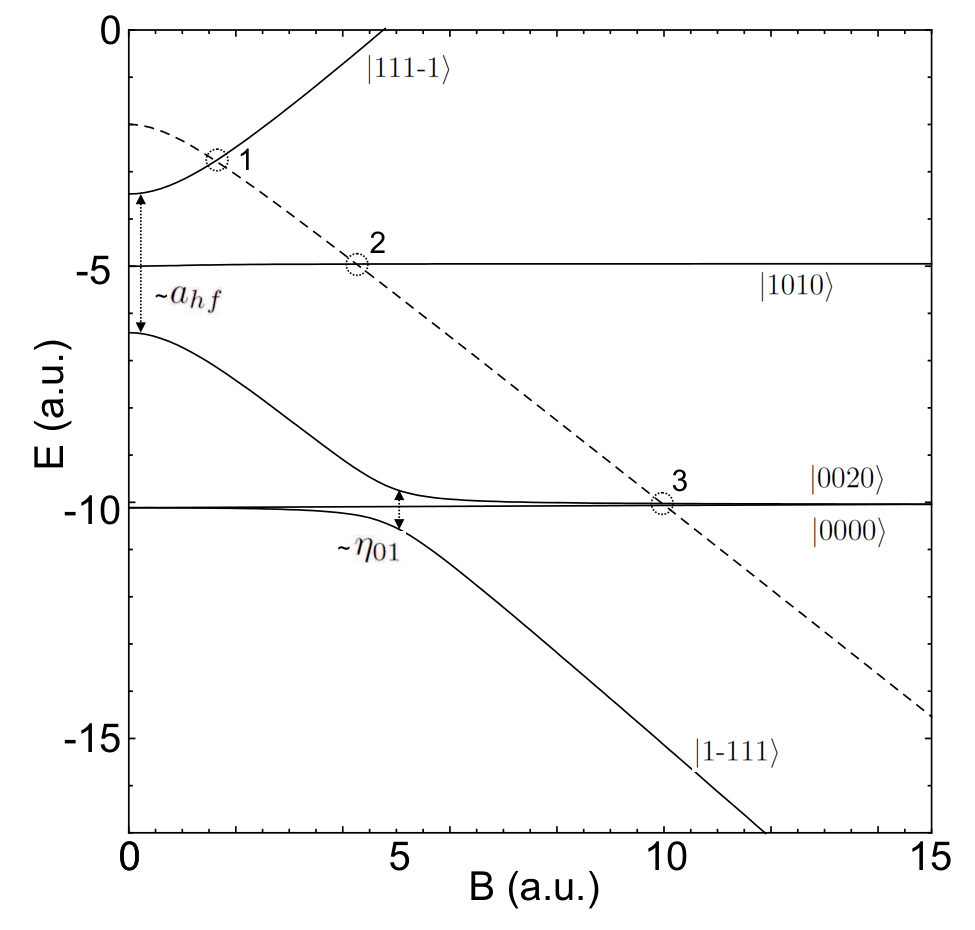
To demonstrate the procedure of identification of Feshbach resonances we show in Fig. 2 the ABM solutions for a simple fictitious homonuclear system with $S=1$ and $I=2$ for an entrance channel with $M_{F}=M_{S}+M_{I}=0$ and $l=0$. The example has the spin structure of ⁶Li but we use ABM parameters, $\epsilon^{0}$, $\epsilon^{1}$ and $\eta^{01}$, with values chosen for convenience of illustration. The field dependence of threshold energy of the entrance channel $E_{\alpha\beta}^{0}$ is shown here explicitly (dashed line). The energies $E_{b}$ (solid lines) are labeled by their high field quantum numbers $|SM_{S}IM_{I}\rangle$ and the binding energies in the singlet and triplet potentials are chosen to be $\epsilon^{0}=-10$ and $\epsilon^{1}=-5$. The avoided crossings around $B=0$ are caused by the hyperfine interaction and is proportional to $a_{\mathrm{hf}}$; the avoided crossing between the singlet and triplet levels is proportional to the wavefunction overlap $\eta^{01}$. Four $s$-wave Feshbach resonances occur indicated at the crossings $1$, $2$ and $3$ (double resonance). The resonances at $1$ and $2$ are mostly determined by the triplet binding energy $\epsilon^{1}$ and the resonances at $3$ by the singlet binding energy $\epsilon^{0}$.

The free parameters of the ABM are the binding energies $\epsilon_{\nu}^{S,l}$ and the Franck-Condon factors $\eta_{\nu,\nu^{\prime}}^{S,S^{\prime}}$. These parameters can be obtained in a variety of manners. Here we discuss three methods, two of which will be demonstrated in Sect. III and the third in Ref. [13].

First, if the scattering potentials $V_{S}^{l}(r)$ are very well known, the bound state wavefunctions of the vibrational levels can be obtained by solving equation (6) for $\epsilon_{\nu}^{Sl}<0$. Numerical values of the Franck-Condon factors follow from the obtained eigenfunctions. This method is very accurate and can be extended to deeply bound levels, however accurate model potentials are only available for a limited number of systems.

A second method can be used when the potentials are not very well or only partially known. For large interatomic distances the potentials can be parameterized by the dispersion potential

Since this expression is not correct for short distances, we account for the inaccurate inner part of the potential by a boundary condition based on the accumulated phase method [15]. This boundary condition has a one-to-one relationship to the interspecies $s$-wave singlet and triplet scattering lengths. This approach requires only three input parameters: the van der Waals $C_{6}$ coefficient and the singlet ($a_{S}$) and triplet ($a_{T}$) scattering lengths. For an accurate description involving deeper bound states the accumulated phase boundary condition can be made more accurate by including additional parameters [15].

The third method to obtain the free parameters is by direct comparison of ABM predictions with experimentally observed Feshbach resonances, for instance obtained in a search for loss features in an ultracold atomic gas. A loss feature spectrum can be obtained by measuring, as a function of magnetic field, the remaining number of atoms after a certain holding time at fixed magnetic field. The ABM parameters follow by a fitting procedure yielding the best match of the predicted threshold crossing fields with the observed loss feature spectrum. We applied this method in Ref. [8], where it has proven to be very powerful for rapid assignment of Feshbach resonances in the ⁶Li-⁴⁰K mixture due to the small computational time required to diagonalize a spin hamiltonian.

The number of fit parameters is determined by the number of bound states which have to be considered. Depending on the atomic species and the magnetic field, only a selected number of vibrational levels $\epsilon_{\nu}^{Sl}$ have to be taken into account. This number can be estimated by considering the maximum energy range involved. An upper bound results from comparing the maximum dissociation energy of the least bound vibrational level $D^{\ast}$ with the maximum internal energy of the atom pair $E_{\mathrm{int,max}}$. The maximum dissociation energy of the $\nu$-th vibrational level can be estimated semi-classically [16]

where $\zeta=2\left[\Gamma(1+1/6)/\Gamma(1/2+1/6)\right]\simeq 3.434$ where $\nu$ is counted from the dissociation limit, i.e. $\nu=1$ is the least bound state. The maximum internal energy is given by the sum of the hyperfine splitting of each of the two atoms at zero field, the maximum Zeeman energy for the free atom pair and the maximum Zeeman energy for the molecule

where $E_{hf}^{\alpha,\beta}=a_{hf}^{\alpha,\beta}(i_{\alpha,\beta}+s_{\alpha,\beta})$ and we have neglected the nuclear Zeeman effect. Comparing equations (12) and (13) gives us an expression for the number of vibrational levels $N_{\nu}$ which have to be considered

where $\lceil x\rceil$ denotes the smallest integer not less than the argument $x$. The maximum possible magnetic field $B_{max}$ required to encounter a Feshbach resonance can be estimated from Eq. 12 by neglecting the hyperfine energy as

If the hyperfine energy is comparable or larger than the vibrational level splitting $D^{\ast}$ the expression for $B_{max}$ overestimates the maximum field of the lowest field Feshbach resonance.

The most crucial ABM parameters are the binding energies $\epsilon_{\nu}^{Sl}$. However, for accurate predictions of the Feshbach resonance positions also the Franck-Condon factors have to be accurate. For weakly bound states these factors are mainly determined by the difference in binding energy of the overlapping states, rather than by the potential shape. Therefore good approximations can be made with little knowledge of the scattering potential.

For very-weakly bound states the outer classical turning point $r_{c}$ is found at distances $r_{c}\gg r_{0}$; i.e., far beyond the Van der Waals radius of the interaction potential

These states are called halo states[17]. Because in this case most of the probability density of the wavefunction is found outside the outer classical turning point, these states can be described by a zero-range potential with a wavefunction of the type $\psi(r)\sim e^{-\kappa r}$, where $\kappa=(-2\mu\epsilon/\hbar^{2})^{1/2}$ is the wavevector corresponding to a bound state with binding energy $\epsilon$. The Franck-Condon factor of two halo states with wavevectors $\kappa_{0}$ and $\kappa_{1}$ is given by

This approximation is valid for binding energies $|\epsilon|\ll C_{6}/r_{0}^{6}$.

The calculation of the Franck-Condon factors can be extended to deeper bound states by including the dispersive van der Waals tail. For distances $r\gg r_{X}$, where $r_{X}$ is the exchange radius, the potential is well described by Eq. (11) and the Franck-Condon factors can be calculated by numerically solving the Schrödinger equation (6) for the Van der Waals potential (11) on the interval $r_{X}<r<\infty$ [18]. The exchange radius $r_{X}$ is defined as the distance where the Van der Waals interaction equals the exchange interaction. This method can be used for asymptotic bound states, which we define by the condition $r_{c}>r_{X}$. If even deeper bound states, with $r_{c}<r_{X}$, have to be taken into account, the potential can be extended by including the exchange interaction [19], or by using full model potentials.

To illustrate the high degree of accuracy achieved by using asymptotic bound states we calculate the Franck-Condon factor for a contact potential (halo states), a van der Waals potential (asymptotic bound states) and a full model potential including short range behavior, derived from Refs. [20, 21]. Figure 3 shows the Franck-Condon factor $\eta_{11}^{01}$ for ⁶Li-⁴⁰K calculated numerically for the model potential, van der Waals potential, and analytically using equation (17). The van der Waals coefficient used is $C_{6}=2322E_{h}a_{0}^{6}$ [22], where $E_{h}=4.35974\times 10^{-18}\penalty\ \mathrm{J}$ and $a_{0}=0.05291772\penalty\ \mathrm{nm}$. The value of $\eta_{11}^{01}$ has been plotted as a function of the triplet binding energy $\epsilon^{1}$ for three different values of the singlet binding energy $\epsilon^{0}$. It is clear that the contact potential is only applicable for $\epsilon/h\lesssim 100$MHz, hence only for systems with resonant scattering in the singlet and triplet channels.

The approximation based on the $C_{6}$ potential yields good agreement down to binding energies of $\epsilon/h\lesssim 40$GHz, which is much more than the maximum possible vibrational level splitting of the least bound states ($D^{\ast}/h=8.2$GHz), hence is sufficient to describe Feshbach resonances originating for the least bound vibrational level. The black circle indicates the actual Franck-Condon factor for the least bound state of ⁶Li-⁴⁰K. For the contact, van der Waals and model potentials we find $\eta_{11}^{01}=0.991$, $\eta_{11}^{01}=0.981$ and $\eta_{11}^{01}=0.979$ respectively.

Both ⁶Li and ⁴⁰K have electron spin $s=1/2$, therefore the total electron spin can be singlet $S=0$ or triplet $S=1$. We intend to describe all loss features observed in Ref. [8]. Since all these features were observed for magnetic fields below $300\penalty\$G we find that, by use of Eq. (14), it is sufficient to take into account only the least bound state ($\nu=1$) of the singlet and triplet potentials. This reduces the number of fit parameters to $\epsilon_{\nu}^{Sl}=\epsilon_{1}^{0,l}$ and $\epsilon_{1}^{1,l}$. Subsequently, we calculate the rotational shifts by parameterizing the $l>0$ bound state energies with the aid of model potentials ²² 2 Note that this procedure can also be applied with only a $C_{6}$ coefficient by utilizing the accumulated phase method. as described by [20, 21] . This allows us to reduce the number of binding energies to be considered to only two: $\epsilon_{1}^{0,0}\equiv\epsilon^{0}$ and $\epsilon_{1}^{1,0}\equiv\epsilon^{1}$. We now turn to the Franck-Condon factor $\eta_{11}^{01}$ of the two bound states. As discussed in Section II.6 its value is $\eta_{11}^{01}=0.979$ and can be taken along in the calculation or approximated as unity. We first consider the case of $\eta_{11}^{01}\equiv 1$, this reduces the total number of fit parameters to only two. We fit the positions of the threshold crossings to the 13 observed loss features reported in Ref. [8] by minimizing the $\chi^{2}$ value while varying $\epsilon^{0}$ and $\epsilon^{1}$. We obtain optimal values of $\epsilon^{0}/h=716(15)\penalty\ \mathrm{MHz}$ and $\epsilon^{1}/h=425(5)\penalty\ \mathrm{MHz}$, where the error bars indicate one standard deviation. In Fig. 4, the threshold and spectrum of coupled bound states with $M_{F}=+3(-3)$ is shown for positive (negative) magnetic field values. The color scheme indicates the admixture of singlet and triplet contributions in the bound states. Feshbach resonances will occur at magnetic fields where the energy of the coupled bound states and the scattering threshold match. The strong admixture of singlet and triplet contributions at the threshold crossings emphasizes the importance of including the singlet-triplet mixing term $\mathcal{H}_{\mathrm{hf}}^{-}$ in the Hamiltonian. All 13 calculated resonance positions have good agreement with the coupled channel calculations as described in Ref. [8], verifying that the ABM yields a good description of the threshold behavior of the ⁶Li$-^{40}$K system for the studied field values.

We repeat the $\chi^{2}$ fitting procedure now including the numerical value of the overlap. The value of $\eta^{01}_{11}$ for both the $s$-wave and $p$-wave bound states are calculated numerically while varying $\epsilon^{0}$ and $\epsilon^{1}$. This fit results in a slightly larger $\chi^{2}$ value with corresponding increased discrepancies in the resonance positions. However, all of the calculated resonance positions are within the experimental widths of the loss features. Therefore, the analysis with $\eta^{01}_{11}\equiv 1$ and $\eta^{01}_{11}=0.979$ can be safely considered to yield the same results within the experimental accuracy.

We now turn to the ⁴⁰K -⁸⁷Rb mixture to demonstrate the application of the ABM to a system including multiple (three) vibrational levels in each potential and the corresponding non-trivial values for the Franck-Condon factors. We consider $s$-wave ($l=0$) resonances. Although accurate K-Rb scattering potentials are known [23], we choose to use the accumulated phase method as discussed in Section II.5 using only three ABM parameters to demonstrate the accuracy of the ABM for a more complex system like ⁴⁰K -⁸⁷Rb.

We solve the reduced radial wave equation (6) for $V_{S}(r)=-C_{6}/r^{6}$ and the continuum state $E=\hbar^{2}k^{2}/2\mu$ in the limit $k\rightarrow 0$. We obtain the accumulated phase boundary condition at $r_{in}=18\penalty\ a_{0}$ from the boundary condition at $r\rightarrow\infty$ using the asymptotic $s$-wave scattering phase shift $\delta_{0}=\arctan(-ka)$, where $a$ is the known singlet or triplet scattering length. Subsequently, we obtain binding energies for the three last bound states of the singlet and triplet potential by solving the same equation (6) but now using the accumulated phase at $r=r_{in}$ and $\psi(r\rightarrow\infty)=0$ as boundary conditions. We numerically calculate the Franck-Condon factors by normalizing the wavefunctions for $r_{in}<r<r_{\infty}$, thereby neglecting the wavefunction in the inner part of the potential ($0<r<r_{in}$). This approximation becomes less valid for more deeply bound states. We use as input parameters $C_{6}=4274\penalty\ E_{h}a_{0}^{6}$ [22], $a_{S}=-111.5\penalty\ a_{0}$ and $a_{T}=-215.6\penalty\ a_{0}$ [23]. Figure 5 shows the spectrum of bound states with respect to the threshold energy for the spin mixture of $|f,m_{f}\rangle=|9/2,-9/2\rangle_{\mathrm{K}}$ and $|1,1\rangle_{\mathrm{Rb}}$ states. The red curves indicate the ABM results and the blue curves correspond to full coupled channel calculations [24]. The agreement between the two models is satisfactory, especially for the weakest bound states close to the threshold. A conceptually different analysis of the K-Rb system using also only three input parameters has been performed by Hanna, et al. [7].

The asymptotic bound state model has been used so far to determine the position of the Feshbach resonances but not their width. As is well known from standard Feshbach theory, the width of $s$-wave resonances depends on the coupling between the resonant level and the continuum [25, 26]. For resonances with $l>0$ the width is determined by a physically different process, namely tunneling through the centrifugal barrier. Here we discuss only the width of $s$-wave resonances. We determine the resonance width by analyzing the shift of the resonant level close to threshold due to the coupling with the least bound state of the open channel. This is possible using again the restricted basis set of bound states $\{|\psi_{\nu}^{Sl}\rangle|\sigma\rangle\}$, introduced in Section II. The possibility to obtain the resonance width by analyzing the shift is plausible because near a resonance the scattering behavior in the zero energy limit is closely related to the threshold behavior of the bound-state. To reveal the coupling as contained in the ABM approximation we partition the total Hilbert space of the Hamiltonian (1) into two orthogonal subspaces $\mathcal{P}$ and $\mathcal{Q}$. The states of the open channels are located in $\mathcal{P}$ space, those of the closed channels in $\mathcal{Q}$ space [10]. This splits the Hamiltonian $\mathcal{H}$ in four parts (cf. Section IV.2); $\mathcal{H}=\mathcal{H}_{PP}+\mathcal{H}_{PQ}+\mathcal{H}_{QP}+\mathcal{H}_{QQ}$. Here $\mathcal{H}_{PP}$ and $\mathcal{H}_{QQ}$ describe the system within each subspace and $\mathcal{H}_{PQ}(=\mathcal{H}_{QP}^{\dagger})$ describe the coupling between the $\mathcal{P}$ and $\mathcal{Q}$ spaces, thus providing a measure for the coupling between the open channels in $\mathcal{P}$ space and the closed channels in $\mathcal{Q}$ space.

The scattering channels are defined by the Breit-Rabi pair states $|\alpha\beta\rangle=|f_{\alpha}m_{f_{\alpha}},f_{\beta}m_{f_{\beta}}\rangle$. In the associated pair basis the diagonal matrix elements of the Hamiltonian $\mathcal{H}$ correspond to the ’bare’ binding energies of the pair states; i.e. the binding energy in the abscence of coupling between the channels by $V(r)$. Restricting ourselves, for purposes of introduction, to a single open channel and to the least bound states in the interaction potentials, $\mathcal{H}_{PP}$ is a single matrix element on the diagonal of $\mathcal{H}$, corresponding to the bare binding energy of the least bound state of the entrance channel, $\epsilon_{P}=-\hbar^{2}\kappa_{P}^{2}/2\mu$. The energy $\epsilon_{P}$ can be readily calculated by projecting the pair state on the spin basis $\{|\sigma\rangle=|SM_{s}\mu_{\alpha}\mu_{\beta}\rangle\}$, and is given by

In the following sections we will show that the width $\Delta B$ of the resonance is a function of the bare binding energy $\epsilon_{P}$ of the entrance channel and a single matrix element of $\mathcal{H}_{PQ}$, denoted by $\mathcal{K}$, representing the coupling of the level $\epsilon_{P}$ to the resonant level in $\mathcal{Q}$ space. We will show that the width is given by the expression

Hence, once the ABM parameters are known, the width of the resonances follows with an additional unitary transformation of the ABM matrix to obtain the coupling coefficient $\mathcal{K}$. In view of the orthogonality of the subspaces $\mathcal{P}$ and $\mathcal{Q}$, the submatrix $\mathcal{H}_{QQ}$, corresponding to all closed channels, can be diagonalized, leaving $\mathcal{H}_{PP}$ unaffected but changing the $\mathcal{H}_{PQ}$ and $\mathcal{H}_{QP}$ submatrices. In diagonalized form the $\mathcal{H}_{QQ}$ submatrix contains the energies $\epsilon_{Q}$ of all bound levels in $\mathcal{Q}$ space and includes the coupling of all channels except the coupling to $\mathcal{P}$ space. This transformation allows to identify the resonant bound state and the corresponding off-diagonal matrix element $\mathcal{K}$ in $\mathcal{H}_{PQ}$, which is a measure for the resonance width. Thus we can obtain the coupling between the open and closed channels without the actual use of continuum states.

In Section IV.2 we present the Feshbach theory tailored to suit the ABM. We give a detailed description of the resonant coupling, and demonstrate with a two-channel model how the ABM bound state energy $E_{b}$ compares to the associated $\mathcal{P}$-space bare energy $\epsilon_{P}$, and to the dressed level in the entrance channel from which one can deduce the resonance width. In Section IV.3 we generalize the results such that the width of the Feshbach resonances can be obtained for the general multi-channel case. For a more thorough treatment of the Feshbach formalism we refer the reader to [25, 26] and for its application to cold atom scattering e.g. [10].

By introducing the projector operators $P$ and $Q$, which project onto the subspaces $\mathcal{P}$ and $\mathcal{Q}$, respectively, the two-body Schrödinger equation can be split into a set of coupled equations [10]

where $|\Psi_{P}\rangle\equiv P|\Psi\rangle$, $|\Psi_{Q}\rangle\equiv Q|\Psi\rangle$, $\mathcal{H}_{PP}\equiv P\mathcal{H}P$, $\mathcal{H}_{PQ}\equiv P\mathcal{H}Q$, etc. Within $\mathcal{Q}$ space the Hamiltonian $\mathcal{H}_{QQ}$ is diagonal with eigenstates $|\phi_{Q}\rangle$ corresponding to the two-body bound state with eigenvalues $\epsilon_{Q}$. The energy $E=\hbar^{2}k^{2}/2\mu$ is defined with respect to the open channel dissociation threshold.

We consider one open channel and assume that near a resonance it couples to a single closed channel. This allows us to write the $S$ matrix of the effective problem in $\mathcal{P}$ space as [10]

where $|\Psi_{P}^{+}\rangle$ are scattering eigenstates of $\mathcal{H}_{PP}$, $S_{P}(k)$ is the direct scattering matrix describing the scattering process in $\mathcal{P}$ space in the absence of coupling to $\mathcal{Q}$ space.

The complex energy shift $\mathcal{A}(E)$ describes the dressing of the bare bound state $|\phi_{Q}\rangle$ by the coupling to the $\mathcal{P}$ space and is represented by

where $E^{+}=E+i\delta$ with $\delta$ approaching zero from positive values. Usually the open channel propagator $[E^{+}-\mathcal{H}_{PP}]^{-1}$ is expanded to a complete set of eigenstates of $\mathcal{H}_{PP}$, where the dominant contribution comes from scattering states. To circumvent the use of scattering states we expand the propagator to Gamow resonance states, which leads to a Mittag-Leffler expansion [27]

where $n$ runs over all poles of the $S_{P}$ matrix. The Gamow state $|\Omega_{n}\rangle$ is an eigenstate of $\mathcal{H}_{PP}$ with eigenvalue $\epsilon_{P_{n}}=\hbar^{2}k_{n}^{2}/(2\mu)$. Correspondingly, the dual state $|\Omega_{n}^{D}\rangle\equiv|\Omega_{n}\rangle^{*}$, is an eigenstate of $\mathcal{H}_{PP}^{\dagger}$ with eigenvalue $(\epsilon_{P_{n}})^{*}$. Using these dual states, the Gamow states form a biorthogonal set such that $\langle\Omega_{n}^{D}|\Omega_{n^{\prime}}\rangle=\delta_{nn^{\prime}}$. For bound-state poles $k_{n}=i\kappa_{n}$, where $\kappa_{n}>0$, Gamow states correspond to properly normalized bound states.

We assume the scattering in the open channel is dominated by a single bound state ($k_{n}=i\kappa_{P}$). This allows us to write the direct scattering matrix in Eq. (22) as

where $a_{\mathrm{bg}}$ is the open channel scattering length, and the $P$-channel background scattering length $a_{\mathrm{bg}}^{P}$ is on the order of the range of the interaction potential $a_{\mathrm{bg}}^{P}\approx r_{0}$. Since we only have to consider one bound state pole (with energy $\epsilon_{P}$) in $\mathcal{P}$ space, the Mittag-Leffler series Eq. (24) is reduced to only one term. Therefore, the complex energy shift Eq. (23) reduces to

where $\mathrm{A}\equiv\langle\phi_{Q}|\mathcal{H}_{QP}|\Omega_{P}\rangle\langle\Omega_{P}^{D}|\mathcal{H}_{PQ}|\phi_{Q}\rangle$ is a positive constant. The coupling matrix element between open-channel bound state and the closed-channel bound state responsible for the Feshbach resonance is related to $\mathrm{A}$.

The complex energy shift can be decomposed into a real and imaginary part such that $\mathcal{A}(E)=\Delta_{\mathrm{res}}(E)-\frac{i}{2}\Gamma(E)$. For energies $E>0$ the unperturbed bound state becomes a quasi-bound state: its energy undergoes a shift $\Delta_{\mathrm{res}}$ and acquires a finite width $\Gamma$. For energies below the open-channel threshold, i.e. $E<0$, $\mathcal{A}(E)$ is purely real and $\Gamma(E)=0$. In the low-energy limit, $k\rightarrow 0$, Eq. (26) reduces to

where $C$ is a constant characterizing the coupling strength between $\mathcal{P}$ and $\mathcal{Q}$ space [10], given by $C=\mathrm{A}(2\kappa_{P}|\epsilon_{P}|)^{-1}$ and $\Delta=\mathrm{A}(2|\epsilon_{P}|)^{-1}$. Note that if the direct interaction is resonant, $|a_{\mathrm{bg}}|\gg r_{0}$, the energy dependence of the complex energy shift is given by [28] $\mathcal{A}(E)=\Delta-iCk(1+ika^{P})^{-1}$ where $a^{P}=\kappa_{P}^{-1}$, yielding an energy dependence of the resonance shift.

Since we consider one open channel, the (elastic) $S$-matrix element can be written as $e^{2i\delta(k)}$, where $\delta(k)$ is the scattering phase shift. The scattering length, defined as the limit $a\equiv-\tan\delta(k)/k,\,(k\rightarrow 0)$, is found to be Eq. (3) which shows the well known dispersive behavior. The direct scattering process is described by the scattering length $a_{\mathrm{bg}}=a_{\mathrm{bg}}^{P}+a^{P}$. At magnetic field value $B_{0}$, where the dressed bound state crosses the threshold of the entrance channel, the scattering length has a singularity.

The dressed state can be considered as a (quasi-) bound state of the total scattering system. The energy of these states is obtained by finding the poles of the total $S$ matrix Eq. (22). This results in solving

for $k$. Due to the underlying assumptions, this equation is only valid for energies around threshold where the open and closed channel poles dominate. Near threshold, the shifted energy of the uncoupled molecular state, $\epsilon_{Q}+\Delta$, can be approximated by $\mu_{rel}(B-B_{0})$. This allows to solve Eq. (28) for $E$ and we readily obtain

retrieving the characteristic quadratic threshold behavior of the dressed level as a function of ($B-B_{0}$). The energy dependence of molecular state close to resonance is also given by $E=-\hbar^{2}/(2\mu a^{2})$ this allows us to express the field width of the resonance as $\Delta B=C(a_{\mathrm{bg}}\mu_{rel})^{-1}$.

We apply the above Feshbach theory to a (fictitious) two-channel version of ABM, and the results are shown in Fig. 6. This two-channel system is represented by a symmetric $2\times 2$ Hamiltonian matrix, where there is only one open and one closed channel. The open and closed channel binding energies $\epsilon_{P}$ resp. $\epsilon_{Q}$ are given by the diagonal matrix elements, while the coupling is represented by the (identical) off-diagonal matrix elements. The closed channel bound state is made linearly dependent on the magnetic field, while the coupling is taken constant. In addition to $\epsilon_{P}$ and $\epsilon_{Q}$, we plot the corresponding ABM solution, which in this case is equivalent to a typical two-level avoided crossing solution. The figure now nicely illustrates the evolution from ABM to the dressed ABM approach, where the latter solutions are found from the two physical solutions of Eq. (28), which are also plotted. Since the dressed ABM solutions account for threshold effects, they show the characteristic quadratic bending towards threshold as a function of magnetic field. From this curvature the resonance width can be deduced.

To illustrate the presented model for a realistic case, we will discuss the ⁶Li-⁴⁰K system prepared in the $|f_{\mathrm{Li}}m_{f_{\mathrm{Li}}},f_{\mathrm{K}}m_{f_{\mathrm{K}}}\rangle=|1/2,+1/2,9/2,-7/2\rangle$ two-body hyperfine state as an example throughout this section. This particular mixture is the energetically lowest spin combination of the $M_{F}=-3$ manifold, allowing to consider only one open channel. We note that the model can be utilized to cases containing more open channels.

In order to calculate the width of a Feshbach resonance using the method presented in Sect. IV.2 three quantities are required: the binding energy of the open channel $\epsilon_{P}$, of the closed channel responsible for the Feshbach resonance $\epsilon_{Q}$, and the coupling matrix element $\mathcal{K}$ between the two channels. In the following we will describe how to obtain these quantities from the ABM by two simple basis transformations.

For ultracold collisions the hyperfine and Zeeman interactions determine the threshold of the various channels and thus the partitioning of the Hilbert space into subspaces $\mathcal{P}$ and $\mathcal{Q}$, and therefore a natural basis for our tailored Feshbach formalism consists of the eigenstates of $\mathcal{H}^{\mathrm{int}}$. Experimentally a system is prepared in an eigenstate $|\alpha\beta\rangle$ of the internal Hamiltonian $\mathcal{H}^{\mathrm{int}}$, which we refer to as the entrance channel (cf. Section II.1). Performing a basis transformation from the ${|\sigma\rangle}$ basis to the pair basis ${|\alpha\beta\rangle}$ allows us to identify the open and closed channel subspace. The open channel has the same spin-structure as the entrance channel.

We now perform a second basis transformation which diagonalizes within $\mathcal{Q}$ space without affecting $\mathcal{P}$ space. We obtain the eigenstates of $\mathcal{H}_{QQ}$ and are able to identify the bound state responsible for a particular Feshbach resonance. The bare bound states of $\mathcal{Q}$ space are defined as $\{|\phi_{Q_{1}}\rangle,|\phi_{Q_{2}}\rangle,\ldots\}$ with binding energies $\{\epsilon_{Q_{1}},\epsilon_{Q_{2}},\ldots\}$. For the one dimensional $\mathcal{P}$ space, which is unaltered by this transformation, the bare bound state $|\Omega_{P}\rangle$ of $\mathcal{H}_{PP}$ is readily identified with binding energy $\epsilon_{P}$. In the basis of eigenstates of $\mathcal{H}_{PP}$ and $\mathcal{H}_{QQ}$ we easily find the coupling matrix elements between the $i$-th $\mathcal{Q}$ space bound state and the open channel bound state $\langle\phi_{Q_{i}}|\mathcal{H}_{QP}|\Omega_{P}\rangle$. This gives the coupling constant $\mathrm{A_{i}}=\langle\phi_{Q_{i}}|\mathcal{H}_{QP}|\Omega_{P}\rangle\langle\Omega_{P}^{D}|\mathcal{H}_{PQ}|\phi_{Q_{i}}\rangle=\mathcal{K}^{2}$ that determines the resonance field $B_{0}$ by solving Eq. (28) at threshold,

The field width of this Feshbach resonance is proportional to the magnetic field difference between the crossings of the dressed ($B_{0}$) and uncoupled $\mathcal{Q}$ bound states ($\widetilde{B}_{0}$) with threshold since

We illustrate the dressed ABM for ⁶Li-⁴⁰K in Figs. 7 and 8, for $M_{F}=-3$. To demonstrate the effect of $\mathcal{H}_{PQ}$, we plotted for comparison both the uncoupled and dressed bound states ³³ 3 For clarity only one of the two physical solutions is shown.. Details of near-threshold behavior (gray shaded area in Fig. 7) are shown in Fig. 8 together with the obtained scattering length. We solved the pole equation of the total $S$-matrix Eq. (28) for each $Q$-state and plotted only the physical solutions which cause Feshbach resonances. The dressed bound states show the characteristic quadratic bending near the threshold. We have used $C_{6}$ to determine $r_{0}$ ($\approx a_{\mathrm{bg}}^{P}$) from Eq. 16.

Table 1 summarizes the results of the dressed ABM for the ⁶Li-⁴⁰K mixture. Note that the position of the Feshbach resonances will be slightly different compared to the results from the regular ABM, for equal values of $\epsilon_{\nu}^{S,0}$. Therefore, we have again preformed a $\chi^{2}$ analysis and we found new values of the binding energies $\epsilon^{0}/h=713\penalty\ \mathrm{MHz}$ and $\epsilon^{1}/h=425\penalty\ \mathrm{MHz}$, which yields a lower $\chi^{2}$ minimum as compared to the regular ABM calculation.

The obtained value of $\Delta B$ generally underestimates the field width of a resonance. This originates from the fact that only the dominant bound state pole corresponding to $a^{P}$ has been taken into account. By including the pole of the dominant virtual state in the Mittag-Leffler expansion, the coupling between the open and closed channel will increase, hence, $\Delta B$ will increase.

References

- [1] For reviews see Proceedings of the International School of Physics “Enrico Fermi,” Course CLXIV, Varenna, 20–30 June 2006, M. Inguscio, W. Ketterle, and C. Salomon (Eds.), IOS Press, Amsterdam, 2008.
- [2] I. Bloch, J. Dalibard, and W. Zwerger, Reviews of Modern Physics 80, 885 (pages 80) (2008), URL http://link.aps.org/abstract/RMP/v80/p885.
- [3] C. Chin, R. Grimm, P. Julienne, and E. Tiesinga, Rev. Mod. Phys. 82, 1225 (2010).
- [4] H. T. C. Stoof, J. M. V. A. Koelman, and B. J. Verhaar, Phys. Rev. B 38, 4688 (1988).
- [5] M. Houbiers, H. T. C. Stoof, W. I. McAlexander, and R. G. Hulet, Phys. Rev. A 57, R1497 (1998).
- [6] J. M. Vogels, B. J. Verhaar, and R. H. Blok, Phys. Rev. A 57, 4049 (1998).
- [7] T. M. Hanna, E. Tiesinga, and P. S. Julienne, Physical Review A (Atomic, Molecular, and Optical Physics) 79, 040701 (pages 4) (2009), URL http://link.aps.org/abstract/PRA/v79/e040701.
- [8] E. Wille, F. M. Spiegelhalder, G. Kerner, D. Naik, A. Trenkwalder, G. Hendl, F. Schreck, R. Grimm, T. G. Tiecke, J. T. M. Walraven, et al., Phys. Rev. Lett. 100, 053201 (2008).
- [9] T. G. Tiecke, M. R. Goosen, A. Ludewig, S. D. Gensemer, S. Kraft, S. J. J. M. F. Kokkelmans, and J. T. M. Walraven, Phys. Rev. Lett. 104, 053202 (2010).
- [10] A. J. Moerdijk, B. J. Verhaar, and A. Axelsson, Phys. Rev. A 51, 4852 (1995).
- [11] C. A. Stan, M. W. Zwierlein, C. H. Schunck, S. M. F. Raupach, and W. Ketterle, Phys. Rev. Lett. 93, 143001 (2004).
- [12] P. Julienne, Private communication (2009).
- [13] M. Goosen, T. Tiecke, W. Vassen, and S. Kokkelmans, in preparation (2010).
- [14] E. Tiesinga, A. J. Moerdijk, B. J. Verhaar, and H. T. C. Stoof, Phys. Rev. A 46, R1167 (1992).
- [15] B. J. Verhaar, E. G. M. van Kempen, and S. J. J. M. F. Kokkelmans, Physical Review A (Atomic, Molecular, and Optical Physics) 79, 032711 (pages 11) (2009), URL http://link.aps.org/abstract/PRA/v79/e032711.
- [16] R. J. LeRoy and R. B. Bernstein, The Journal of Chemical Physics 52, 3869 (1970), URL http://link.aip.org/link/?JCP/52/3869/1.
- [17] A. S. Jensen, K. Riisager, D. V. Fedorov, and E. Garrido, Rev. Mod. Phys. 76, 215 (2004).
- [18] B. Gao, Phys. Rev. A 58, 1728 (1998), describes analytical solutions.
- [19] B. M. Smirnov and M. I. Chibisov, JETP 21, 624 (1965).
- [20] H. Salami, A. J. Ross, P. Crozet, W. Jastrzebski, P. Kowalczyk, and R. J. L. Roy, The Journal of Chemical Physics 126, 194313 (pages 9) (2007), URL http://link.aip.org/link/?JCP/126/194313/1.
- [21] M. Aymar and O. Dulieu, The Journal of Chemical Physics 122, 204302 (pages 9) (2005), URL http://link.aip.org/link/?JCP/122/204302/1.
- [22] A. Dervianko, J. F. Babb, and A. Dalgarno, Phys. Rev. A 63, 052704 (2001).
- [23] A. Pashov, O. Docenko, M. Tamanis, R. Ferber, H. Knöckel, and E. Tiemann, Physical Review A (Atomic, Molecular, and Optical Physics) 76, 022511 (pages 10) (2007), URL http://link.aps.org/abstract/PRA/v76/e022511.
- [24] J. P. S., Faraday Discussions 142, 361 (2009).
- [25] H. Feshbach, Ann. Phys. 5, 357 (1958).
- [26] H. Feshbach, Ann. Phys. 19, 287 (1962).
- [27] B. Marcelis, E. G. M. van Kempen, B. J. Verhaar, and S. J. J. M. F. Kokkelmans, Phys. Rev. A 70, 012701 (2004).
- [28] B. Marcelis and S. J. J. M. F. Kokkelmans, Phys. Rev. A 74, 023606 (2006).
- [29] A.-C. Voigt, M. Taglieber, L. Costa, T. Aoki, W. Wieser, T. W. Hänsch, and K. Dieckmann, Phys. Rev. Lett. 102, 020405 (2009).
- [30] F. M. Spiegelhalder, A. Trenkwalder, D. Naik, G. Kerner, E. Wille, G. Hendl, F. Schreck, and R. Grimm, Phys. Rev. A 81, 043637 (2010).
- [31] T. V. Tscherbul, T. Calarco, I. Lesanovsky, R. V. Krems, A. Dalgarno, and J. Schmiedmayer, Phys. Rev. A 81, 050701 (2010).
- [32] C. Chin, T. Kraemer, M. Mark, J. Herbig, P. Waldburger, H.-C. Nägerl, and R. Grimm, Phys. Rev. Lett. 94, 123201 (2005).