Narrowband Biphoton Generation due to Long-Lived Coherent Population Oscillations

Traditionally, paired photons are produced from spontaneous parametric down conversion in nonlinear crystals. The bandwidth of such biphotons is very broad and typically in the terahertz range [1], which makes them useless for some applications in quantum information science which require strong interaction between photons and atomic systems. This problem can be overcome by generating biphotons in cold atomic systems which have a narrowband nonlinear response. For example, biphotons can be produced when a double-$\Lambda$ system [2, 3, 4] or two-level system (TLS) [5, 6] is pumped by two counter-propagating laser fields. Then phase-matched and energy-time entangled photon pairs are produced due to the effect of four-wave mixing (FWM). Biphotons from a such source have a bandwidth in the megahertz range and coherence time of hundreds of nanoseconds.

In this paper, we demonstrate that narrowband biphotons can also be produced due to the effect of long-lived coherent population oscillations (CPOs) in a TLS with an intermediate metastable state. In such a system, the width of the nonlinear response is determined by the lifetime of the metastable state, which can vary significantly depending on the nature of the quantum system. For example, in semiconductor quantum wells and dots [7] the CPO lifetime is in the microsecond range, whereas in a ruby crystal [8] or organic film [9] it can be more than a millisecond, leading to a broad range of potential applications of photon pairs based on the CPO effect.

We consider the interaction of an ensemble of TLSs that decay via a single intermediate metastable state with two counterpropagating pump fields with amplitude $E_{0}$ (see Fig.1). The medium is assumed to be optically thin in the direction of pump propagation and the effect of pump depletion is not taken into account. Due to pumping of the TLS by two counter-propagating laser fields, photon pairs are produced [5, 6] where photons from the same pair also counter-propagate so that the phase-matching condition of FWM is satisfied [10] [see Fig. 1(a)] (actually, in such a configuration biphotons are emitted into the whole $4\pi$ space). In order to allow for the spontaneous initiation process, the generated weak fields are described by quantum-mechanical operators

where the subscript $1$ denotes the field at frequency $\omega_{1}=\omega_{0}+\delta$ propagating along the positive z-axis, and the subscript $2$ denotes the field at frequency $\omega_{2}=\omega_{0}-\delta$ moving along the negative z-axis, $E_{1,2}^{\left(0\right)}=\left(\hbar\omega_{1,2}/2\varepsilon_{0}V\right)^{1/2}$ is the vacuum field, $V$ is the quantization volume, and $\widehat{a}$ and $\widehat{a}^{\dagger}$ are the photon annihilation and creation operators.

To describe the evolution of the atomic ensemble, we begin with the Heisenberg operator equations of the motion in the dipole approximation:

where $\widetilde{\sigma}_{ij}=\left|i\right\rangle\left\langle j\right|$ is the atomic operator, $\widetilde{E}^{\left(\pm\right)}$ is the total field operator, and $d_{ij}$ is the transition dipole matrix element, $\Gamma_{ba}$ is the transverse relaxation rate, $\gamma_{ij}$ is the longitudinal decay rate from the state $\left|i\right\rangle$ to the state $\left|j\right\rangle$, $\gamma_{b}=\gamma_{bc}+\gamma_{ba}$ is the total decay rate from the excited level, and $\Omega=\omega_{0}-\omega_{ba}$ is the pump detuning from the resonance. We also assume that the system is closed so that $\widetilde{\sigma}_{aa}+\widetilde{\sigma}_{bb}+\widetilde{\sigma}_{cc}=1.$

We apply the slowly-varying envelope approximation and write the total field operator as

The pump-probe interaction with a TLS is characterized by population beating or coherent population oscillations (CPOs) at $\delta$, the frequency difference between pump and probe fields [12]. In an ordinary TLS, the CPOs decay at the same rate as the excited state. However, the situation can be quite different if an intermediate metastable state is included [see Fig. 1(b)]. In the case where the rate of transfer of CPO from the excited state to the metastable state is much faster than the rate of transfer of CPO from the excited to the ground state due to population relaxation or pump-induced transitions, that is,

where $V_{0}=d_{ba}E_{0}/\left(2\hbar\right)$ is the pump Rabi frequency which is assumed to be real, long-lived CPOs of ground and metastable states are created [13]. This leads to a narrow dip in the probe absorption spectrum and a narrow peak in the FWM spectrum [13, 14, 15].

Under these conditions and taking into account that level $\left|c\right\rangle$ is the metastable level $\gamma_{ca}\ll\gamma_{ba},\gamma_{bc}$ the steady-state response of the medium to the generated fields is given by [15, 16]

The evolution of the annihilation and creation operators $\widehat{a}$ and $\widehat{a}^{\dagger}$ is described by the coupled propagation equations [4]:

In order to solve these coupled equations we make a Fourier transformation, neglect the term $i\omega/c$ as it does not affect the final result [4], and substitute Eqs. (6a) and (6b) into Eqs. (9a) and (9b) to obtain

where

The correlation between the photons emitted to the left and right is described by the second-order Glauber correlation function $G_{21}^{\left(2\right)}$ [17]

As a field emitted by many statistically independent atoms behaves as a Gaussian random variable, we can use the Gaussian momentum theorem [4, 17] and rewrite Eq. (13) in the form

As seeding fields $\widehat{E}_{1,2}$ are absent, the vacuum field fluctuations determine the initial conditions and taking into account the commutation relation for the input field operators $\left[\widehat{a}_{1,2}\left(z,\omega\right),\widehat{a}_{1,2}^{\dagger}\left(z,-\omega^{\prime}\right)\right]=L/\left(2\pi c\right)\delta\left(\omega+\omega^{\prime}\right)$ in Eqs. (14b) and (14c), we obtain

In particular, we are interested in the biphoton coherence time which is determined by the width of the function $\Phi_{21}\left(\tau\right)$. Harris and coworkers [2] have pointed out that a long coherence time can be obtained due to the effect of slow light [19] experienced by one of the photons of the entangled pair but not by the other. Here we demonstrate that a long coherence time can be obtained even in a optically thin medium

where the time delay between the photons due to the slow light effect is negligible.

Under the conditions of Eq. (16), Eqs. (12a) and (12b) simplify to

To find the analytical form of the correlation function, we substitute Eqs. (17) into Eqs. (15a) and (15b) and integrate over $\delta$:

When Eq. (16) holds, the denominator of the second term of Eq. (19) is much less than unity and as a result the visibility $V_{\text{vis}}=\left(g_{\max}^{\left(2\right)}-g_{\min}^{\left(2\right)}\right)/\left(g_{\max}^{\left(2\right)}+g_{\min}^{\left(2\right)}\right)\approx 1$.

In Fig. (2), we show the behavior of the normalized second-order correlation function. It can be seen that the characteristic width is determined by $1/W$ and also that there is an antibunching-like effect with a characteristic time $1/\Gamma_{ba}$ (red solid line). When the pump detuning is non-zero (blue dotted line), damped oscillations at frequency $\Omega$ with a decay rate $1/\Gamma_{ba}$ are produced.

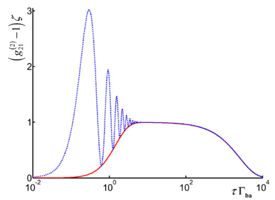
This behavior is easy to understand if we look at Eq. (18b), which shows that the biphoton wave function is a coherent superposition of two different FWM processes [6]. The first term describes the generation of the biphotons with a spectral width $W$ centered at the point $\delta=0$ (we call this $FWM_{I}$) and the second term describes generation of the biphotons with a spectral width $\Gamma_{ba}$ from the two sidebands which are centered at the points $\delta=\pm\Omega$ (called $FWM_{II}$). As we can see from Eq. (18b), the phase shift between $FWM_{I}$ and $FWM_{II}$ oscillates at the frequency of the pump detuning which leads to constructive or destructive interference between them, as shown in Fig. (2). The coherence time of the biphoton generated by $FWM_{II}$ is determined by $1/\Gamma_{ba}$, so that these biphotons can contribute to the coherent superposition only during this period, which causes a fast damping of the oscillations. When the pump detuning is zero, there is always destructive interference between the biphotons from $FWM_{I}$ and $FWM_{II}$, leading to an anti-bunching dip with a width $1/\Gamma_{ba}$ (we should note that the depth of the antibunching dip never goes to zero as we have a macroscopic ensemble of the quantum systems). The long coherence time is caused by biphotons that originate from the $FWM_{I}$ process as it has a very narrow bandwidth [see Eq. (8b)].

In summary, we have demonstrated that the combined effects of FWM and long-lived CPOs in a TLS with intermediate metastable state are able to produce narrowband biphotons with a long coherence time whose maximum value is equal to the lifetime of the metastable state. The biphotons’ waveform and bandwidth can be controlled by the pump intensity. During the time $1/\Gamma_{ba}$ the biphoton wavefunction shows antibunching behavior. If the pump field is detuned, damped oscillation during this period is observed.

The authors thank A. Pe’er and A. Eilam for helpful discussions.

References

- [1] A. Yariv and P. Yeh, Optical Electronics in Modern Communication (Oxford University Press, 2007).
- [2] V. Balic et al. Phys. Rev. Lett. 94, 183601 (2005); P. Kolchin et al. Phys. Rev. Lett. 97, 113602 (2006); S. Du et al. Phys. Rev. Lett. 100, 183603 (2008).
- [3] C.H. van der Wal et al. Science 301, 196 (2003); A. Kuzmich et al. Nature (London) 423, 731 (2003); J.K. Thompson et al. Science 313, 74 (2006); S. Du, J. Wen, and M. Rubin, J. Opt. Soc. Am. B 12, C98 (2008).
- [4] C.H.R. Ooi, et al. Phys. Rev. A 75, 013820 (2007); P. Kolchin, Phys. Rev. A 75, 033814 (2007).
- [5] P. Grangier, et al. Phys. Rev. Lett. 57, 687 (1986).
- [6] S. Du et al. Phys. Rev. Lett. 98, 053601 (2007); J. Wen, S. Du, and M. Rubin, Phys. Rev. A 75, 033809 (2007); J. Wen et al. Phys. Rev. A 78, 033801 (2008).
- [7] P.C. Ku, C.J. Chang-Hasnain, and S.L. Chuang, J. Phys. D: Appl. Phys. 40, R93 (2007).
- [8] L.W. Hillman, et al., Opt. Commun. 45, 416 (1983); M.S. Bigelow, N.N. Lepeshkin, and R.W. Boyd, Science 301, 200 (2003).
- [9] P. Wu and D.V.G.L.N. Rao, Phys. Rev. Lett. 95, 253601 (2005).
- [10] R. W. Boyd, Nonlinear Optics (Academic, San Diego, 2003).
- [11] D. Tannor, Introduction to Quantum Mechanics: A Time Dependent Perspective (University Science Press, Sausalito, 2007).
- [12] E.V. Baklanov and V.P. Chebotaev, Sov. Phys. JETP 33, 300 (1971); M. Sargent III, Phys. Rep. 43, 223 (1978); R. W. Boyd, et al. Phys. Rev. A 24, 411 (1981); R.W. Boyd and M. Sargent III, J. Opt. Soc. Am. B 5, 99 (1988).
- [13] A. Eilam, et al. Opt. Lett. 35, 772 (2010).
- [14] H. Friedmann, A.D. Wilson-Gordon, and M. Rosenbluh, Phys. Rev. A 33, 1783 (1986).
- [15] A.V. Sharypov, et al. Phys. Rev. A 81, 013829 (2010); I. Azuri, et al. Opt. Commun. (2010), doi:10.1016/j.optcom.2010.06.057.
- [16] Yu. I. Heller and A.V. Sharypov, Opt. Spectr. 106, 252 (2009).
- [17] L. Mandel and E. Wolf, Optical Coherence and Quantum Optics (Cambridge University Press, Cambridge England, New York, 1994); D.N. Klyshko, Photons and Nonlinear Optics (Gordon and Breach, 1988).
- [18] M.H. Rubin, et al. Phys. Rev. A 50, 5122 (1994).
- [19] S.E. Harris, J.E. Field, and A. Kasapi, Phys. Rev. A 46, R29 (1992).