Extraction of the resonance parameters at finite times
Abstract
In this paper we propose a model-independent method to extract the resonance parameters on the lattice directly from the Euclidean 2-point correlation functions of the field operators at finite times. The method is tested in case of the two-point function of the -resonance, calculated at one loop in Small Scale Expansion. Further, the method is applied to a -dimensional model with two coupled Ising spins and the results are compared with earlier ones obtained by using Lüscher’s approach.
Keywords:
Unstable states, lattice field theory, Ising modelpacs
05.50.+q, 11.10.St, 11.15.Ha, 12.38.GcI Introduction
It is well known that the asymptotic behavior of the two-point function for large Euclidean times is determined by the lowest eigenvalue of the Hamiltonian in a given channel. In case of stable particles, this property allows one to determine their masses. The case of the excited states is different. Here, the two-point function yields the spectrum of the so-called “scattering states.” The relation to the energy and width of the resonance states is not direct, since a resonance, in general, can not be associated with an isolated energy level of a Hamiltonian. Up to now, several alternative methods have been used to determine these quantities from the lattice Monte Carlo (MC) simulations. These are:
- i)
At present, Lüscher’s approach [1, 2, 3, 4] is widely used to deal with the resonances in lattice QCD, obtained in simulations with sufficiently low quark masses. In brief, the procedure consists in determining first the phase shift by studying the volume dependence of the energy spectrum on the lattice. Then, continuing the -matrix into the complex plane (e.g., by using the effective-range expansion whenever possible), one attempts to determine the position of the poles on the second Riemann sheet. This procedure is described in detail in Ref. [5], where the generalization to the case of the resonance matrix elements (in 1+1 dimensions) is also considered. A shortcut is provided by using Breit-Wigner type parameterization for the scattering phase and determining its parameters (energy and width) from the lattice data (see, e.g. Ref. [6] and Refs. [7, 8], where the method has been applied in the case of the - and -mesons, respectively). The Lüscher’s approach has been also generalized for the moving frames [9].
- ii)
Recently, the spectral functions in QCD have been reconstructed by using the maximal entropy method (see, e.g. [10, 11, 12]). This method, as well as Lüscher’s approach, has in principle the capacity to address the problem of the extraction of the resonance energy and width from the Euclidean MC simulations on the lattice.
- iii)
The Euclidean correlators have been parameterized in terms of the energy and width of an isolated resonance state, in order to subsequently determine these quantities from the fit to the lattice data [13]. In that paper, the method has been applied to study the glueball decay.
- iv)
- v)
Recently, there has been a substantial activity in the determination of the excited meson and baryon spectrum by using generalized eigenvalue equations [23, 22, 16, 17, 18, 19, 20, 21]. Despite spectacular progress achieved in the field, it should be stressed once again that a resonance state can not be uniquely associated with a particular energy level. To a certain extent, excited states and scattering states can be distinguished, e.g., by studying the volume dependence of the spectral density [24, 25]. This method, however works for narrow resonances only [26].
In this paper, we combine some of the above ideas and propose a systematic method to extract resonance pole positions from lattice data. In its present form, our approach is applicable to the systems with a low-lying, well-isolated, narrow resonance in the spectrum (for example, the or the ). First, we have tested our method using synthetic input data, represented by the Euclidean propagator of the , calculated in the low energy effective field theory at one loop. A further test has been carried out in a 1+1 dimensional model of two coupled Ising spins, where the resonance parameters have been determined in the past utilizing Lüscher’s approach [27, 28]. In both cases, we find that the method is capable to extract the pole position of the resonance.
The outline of the paper is as follows. In section II we discuss the foundations of the method. The general representation of the two-point function in the presence of a low-lying isolated resonance is discussed in section III. In section IV we consider the procedure of the data fitting and the determination of the pole position by using synthetic data. A short review of the 1+1 dimensional Ising model is given in section V. The extraction of the resonance pole in this model is considered in section VI. Finally, section VII contains our conclusions. Some technicalities are relegated to the appendices.
II Källen-Lehmann representation
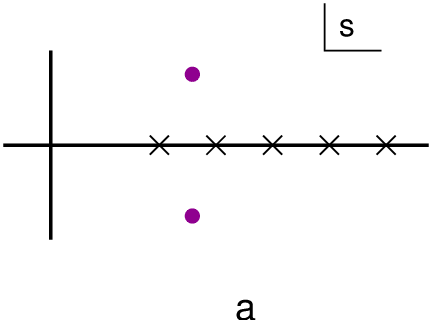

In the beginning of this section, we present a qualitative reasoning to justify our method. We start by mentioning that lattice QCD simulations are always carried out on lattices with a finite (Euclidean) time and spatial extension. Below, we consider lattices of the size , where and denote the box size in time and space, respectively, and is the number of spatial dimensions. For not so large (however, large enough to suppress the polarization effects in stable particles), the energy levels are well separated and can in principle be extracted from the asymptotic behavior of the two-point function at large Euclidean times , where denotes the average level spacing. The Fourier-transform of the two-point function is a meromorphic function in the complex -plane (see Fig. 1a). Consequently, the second Riemann sheet, as well as the poles on it (corresponding to the resonances), do not appear at any finite . The information about these poles stays encoded in the dependence of the spectrum on the spatial box size and can be extracted (in several consecutive steps, as explained in the introduction) by using Lüscher’s approach.
In case an almost stable state is present, such a complicated procedure might seem superfluous. Intuitively, it is clear that, if the decay width is small, the resonance will behave pretty much the same way as a stable particle and will determine the -dependence of the two-point function in a large interval (however, not for the asymptotically large times , when the resonance already has decayed). Consider, for example, a lattice with the large spatial size , and calculate the two-point function at finite (see Fig. 1b). If the “resolution” is larger than the distance between energy levels, the two-point function is given by a sum of (many) exponentials with the spectral weight suppressed by a factor , so that, effectively, the spectral sum transforms into an integral over the energies. This is equivalent to the emergence of the cut that connects the physical sheet to the second sheet. We expect that, in this case, one may find an alternative representation of the two-point function in terms of quasiparticle degrees of freedom corresponding to the pole(s) on the second Riemann sheet (i.e. the resonance decay and width) plus a small background which can be described by a few parameters. Namely, we expect that there exists a window in the variable , where such a description will be more effective than the multi-exponential representation through the energies and spectral weights.
Hence, the original problem is reduced to finding a universal, model-independent parameterization of the two-point function in the presence of a narrow resonance, which will allow one to determine the energy and the width of the latter by performing a fit to the lattice data. This is analogous to the exponential parameterization, which allows one to determine the mass of a stable particle by fitting at asymptotically large times. Note that we shall try to avoid approximations in the spectral function (e.g. the narrow width approximation used in Ref. [13]), which are a potential source of a systematic error. The contribution of the background, albeit small, will be taken into account in a systematic manner.
The model-independent parameterization, which was mentioned above, can be obtained directly by using the Källen-Lehmann representation for the two-point function. Below, we give a brief derivation of this representation in a finite box. Further, we consider the limits and in detail, in order to quantify the qualitative arguments given in the beginning of this section.
In the derivation of the Källen-Lehmann representation in a finite volume, we mainly follow the steps given in Ref. [10]. Let be any local field, carrying the resonance quantum numbers. The two-point function of this field in the Euclidean space is defined as
| (1) |
where the upper (lower) sign corresponds to bosons (fermions). The Fourier transform of this expression takes the form
| (2) |
where , with , are Matsubara frequencies in case of bosons (fermions), and with .
Using a complete set of Hamiltonian eigenvectors to calculate the trace in Eq. (1), one gets
| (3) |
where denotes the periodic Kronecker in dimensions. This relation can be rewritten as
| (4) |
where the spectral function is given by
| (5) |
By applying discrete symmetries, it can be shown that the spectral function obeys the following properties [10]
| (6) |
The dispersion integral can be rewritten as11 1 For illustrative purpose, below we display the bosonic case only. The fermionic case can be treated similarly.
| (7) |
Finally, in the limit , only the vacuum state , contributes, and the spectral function in Eq. (7) is given by
| (8) |
Now, let the variable be outside the narrow strip along the negative real axis. Then, the function for all is uniformly bound from above by some large constant . For fixed , performing the limit and applying the regular summation theorem [29], it is seen22 2 The regular summation theorem implies that the matrix elements are continuous functions of . We examine these matrix elements explicitly in a simple quantum mechanical model in Appendix A and show that in this case the above requirement is indeed fulfilled. that the quantity approaches , with the pertinent spectral function given by
| (9) |
where stands for the sum (integral) over the continuous spectrum wave functions. More precisely, for outside the strip
| (10) |
where is determined by the invariant mass of the lowest-mass state. Further, according to the regular summation theorem, the difference , where
| (11) |
for any and converges faster than any power of as (for a discussion, see Appendix A). In other words, in this limit the two-point function converges to its infinite-volume counterpart everywhere in the complex plane except the narrow strip along the cut (for a related discussion, see also Ref. [30]). This statement is a mathematical formulation for the intuitive picture of “poles merging into the cut,” which is shown in Fig. 1b. To further illustrate this, an example of a function which is meromorphic at a finite and develops a cut and a pole on the second Riemann sheet in the limit , is given in Appendix B.
Moreover, from Eq. (2) one finds
| (12) | |||||
The last line is obtained in the limit . Together with the expression (8) for the spectral density, we recover the representation for as a sum over exponentials. In the case is much larger than the distance between different energy levels (this can be achieved, e.g., by holding fixed and increasing ), many exponentials contribute to and the sum over the energy eigenvalues can be replaced through the integral. In this case, is replaced by .
To summarize, the behavior of the two-point function can be studied in different regimes. For asymptotically large and moderately large , only the few lowest, well-separated energy levels contribute. This situation is well described by a sum of a few exponential terms. In difference to this, in the regime with asymptotically large and moderately large there are many terms with nearly the same energies that contribute to the multi-exponential representation. The sum over the discrete energy spectrum effectively transforms into an integral. If, in addition, a low-lying well separated resonance emerges, we expect that the spectral integral can be efficiently parameterized in terms of the resonance parameters instead of the stable energy levels.
III Two-point function at finite
As discussed in the previous section, it is possible to perform the infinite-volume limit in the two-point function, keeping the Euclidean time fixed. The spectral representation is given by Eq. (7) with the spectral density given by Eq. (9). Note that the spectral density vanishes for , and hence the integration in Eq. (7) in fact is performed from to infinity.
For simplicity, we work in the center-of-mass (CM) frame and denote , . The spectral representation then takes the form
| (13) |
In the vicinity of the elastic threshold, , where stands for the orbital angular momentum33 3 This statement is valid in 3+1 dimensions. In 1+1 dimensions, one has to substitute in all formulae..
Assume now that an isolated low-lying resonance emerges. This is equivalent to the statement that the function takes the form
| (14) |
where the singularities of the function lie far enough from the threshold so that the Taylor expansion of this function converges in the part of the complex plane that includes the resonance poles at and . The energy and the width of the resonance is determined by in the standard manner. Note that these poles come in complex-conjugated pairs44 4 is the discontinuity of a function which is analytic in the cut complex plane and obeys Schwarz reflection principle. Hence the poles in this function (which emerge on the second Riemann sheet), always come in pairs. This is the justification for the ansatz (14)..
Using Eq. (14), it can be easily shown that
| (15) |
where . As mentioned before, it is assumed that the Taylor expansion converges in the part of a complex region which includes the resonance poles.
From the above expression we get
| (16) |
In particular, for , we find
| (17) |
where
| (18) |
and the following representation in form of an infinite series is useful in a wide range of the variable
| (19) |
Further, the functions with can be recursively expressed through . The general representation of the two-point function follows straightforwardly from the above relations
| (20) |
where and are expressed through the Taylor coefficients as well as .
Eq. (20) represents our central result. It provides a universal parameterization of the Euclidean two-point function in the presence of a low-lying isolated resonance described by two parameters . The couplings are associated with the non-resonant background. In particular, it encodes the contribution of the threshold which lies below the resonance energy. This means that if is taken too large, the background dominates and the information about is erased. We assume, however, that in the presence of a narrow resonance, there exists a sufficiently wide window in , where the background is small and can be determined from the fit of the measured to the representation (20). We require that, in this window, adding the background parameterized by the constants should lead to small corrections in and the fit should remain stable against the increase of the number of independent .

The physical meaning of our method can be easily illustrated by Fig. 2. In this figure, the effective mass of a system in the presence of a stable state/resonance is schematically depicted. If there is a stable particle, the plateau in the effective mass sets in almost immediately. However, if a resonance instead of a stable particle is present, there exists a wide window in , where many excited states contribute and the effective mass decreases slowly until it reaches the asymptotic value. Our method roughly corresponds to fitting within this interval by the representation given in Eq. (20), and the decay width is determined by the rate of the decrease of the effective mass. Note that a similar picture was obtained in Ref. [31]. In that paper, the theory of two coupled scalar fields, where the heavier field can decay into a couple of light scalars, was considered. In particular, it has been shown that the effective mass of the heavy scalar, calculated on the lattice, exhibits the same behavior when its mass is below/above the two-particle threshold (see Fig. 1 of that article). The two point functions of the excited mesons in QCD also exhibit a similar behavior [16].
It is instructive to compare the parameterization (20) to the pertinent formula obtained in Ref. [13]. A technical difference consists in the absence of the threshold factor that results in a different parameterization of the background. The important difference is, however, that in Ref. [13] a Breit-Wigner type parameterization for the spectral function is originally assumed. Since this ansatz did not fit the lattice data well, an ad hoc energy-dependence in the decay width has been introduced, and the functional form of this dependence has been determined by using a trial-and-error method. In our approach, the representation of , given in Eq. (20) is completely general and is based on the sole assumption that a well-isolated resonance emerges at low energies. The background is parameterized by the constants in a systematic manner.
IV The fit
We first test our method by using synthetic data. Consider, for instance, the propagator of the -resonance evaluated in the Small Scale Expansion (SSE)55 5 The SSE is a phenomenological extension of Chiral Perturbation Theory in which the -nucleon mass splitting is counted as an additional small parameter. This quantity, however, does not vanish in the chiral limit. The framework of the SSE is laid in detail in Ref. [32]. at one loop [33, 34]. In the Minkowski space, this propagator is given by
| (21) |
where denotes the mass of the -resonance in the chiral limit, stands for the projector onto the spin-3/2 state and the spin-1/2 part does not have a pole in the low-energy region (for a general proof of this statement, see [35]). Further, the invariant functions at order in the chiral expansion are given by
| (22) |
where and denote the coupling constant and the pion decay constant in the chiral limit, respectively, are the nucleon, and pion masses, respectively, and the invariant functions are given by [33, 34]
| (23) |
The trace of obeys the dispersion relation
| (24) |
where the expression for the discontinuity can be directly read off from Eqs. (21)-(23).
In the calculations we have used the following values of the parameters: , , , and (this value leads to the width in a calculation at ). It is easy to check that the propagator has a pole at and (note the large shift in the quantity as compared to its value obtained at that presumably is an artefact of a approximation).
Next, we wish to investigate whether it is possible to recover this result by applying our method. To this end, we analytically continue Eq. (24) into Euclidean space and perform the Fourier transform with respect to the fourth component of the momentum. The resulting values are treated as synthetic data. We choose the interval and perform a least squares fit of these data to the formula (20) (the data points are assumed to be distributed equidistantly in this interval).
In the fit, we cut the sum in Eq. (20) at some value . The fit of the 7 data points with yields and that is already close to the exact values. The procedure converges rapidly. At the accuracy of the digits displayed, the exact result is obtained for . Adding more terms, it is possible to improve the agreement with the exact result up to very many decimal digits.
To summarize, using synthetic data, we have demonstrated that our method is capable to reconstruct the exact position of a pole in a complex plane from a limited data sample. To perform a similar analysis for real Monte Carlo data is much more challenging. One of the main problems that we have encountered there, is related to the instability of the fit when increases (this problem already arises for relatively small ). Namely, the constants , which describe the background, become very large in magnitude having alternating signs and this destabilizes the values of extracted from the fit.
In order to circumvent this problem, we have performed a Bayesian fit to the lattice MC data. A detailed description of the Bayesian fit techniques, which is well suited for our purposes, can be found, e.g. in Ref. [36]. We shall present a brief summary of the method below. The function to be minimized in the standard least squares fit is given by
| (25) |
where are data corresponding to the points . In Eq. (25) it is implicitly assumed that the MC errors in the data do not vary much with . Note that the above form still does not include our prior knowledge about . The assumption about the smoothness of the function in Eq. (14) implies that should be of “natural size” excluding the scenario where the become large with alternating signs.
In order to implement this prior knowledge into the fitting procedure, in analogy with Ref. [36], we define the augmented
| (26) |
where is some scale that ensures that all stay in the “natural” range.
We determine the quantity by using the trial-and-error method. If is too large, the introduction of does not cure the problem with the convergence. This sets the upper limit on the value of . The lower limit for is set by the requirement that the results obtained with standard and agree for low . In addition, within this range, the final result of the fit for should not depend on .
In the 1+1 dimensional model with two Ising spins discussed in the next section, we have performed fits using . Below we show that this technique allows one to extract the precise values of from the lattice MC data in this model.
V dimensional model with two coupled Ising spins
In this section we apply our method to the extraction of the resonance pole position to a 1+1 dimensional model of two coupled Ising spins. This model has been treated in Refs. [27, 28] using Lüscher’s approach. In particular, it has been shown that a narrow resonance emerges in the system, whose parameters can be extracted in a systematic manner.
The action of the model is given by
| (27) |
where are two Ising spins which interact with each other through the Yukawa-type coupling . The sum , where , runs over all lattice points and denotes the unit vector along the spatial axis. The couplings are chosen so that the masses of and are and (in lattice units). Note that, if , the decays into , so corresponds to the resonance energy in this case.
The model has been analyzed in detail in Refs. [27, 28]. We give only a short summary of this analysis here. In particular, it has been argued that in the theory described by the Lagrangian (27) no second-order phase transition occurs and thus the continuum limit can not be performed. In other words, all results obtained here refer to the effective theory with an ultraviolet cutoff.
The energy spectrum is determined by solving the generalized eigenvalue problem. The operator basis is defined as in Refs. [27, 28]
| (28) |
with . The correlator matrix is given by
| (29) |
The spectral decomposition of is approximated by the truncated series
| (30) |
The energy eigenvalues for are determined by diagonalizing the matrix , where is some fixed time (in the following, as in Refs. [27, 28], we always use ). The eigenvalue equation takes the form
| (31) |
where form an orthonormal basis. The eigenvectors are given by .
The MC simulation is done by using a cluster algorithm [37]. We closely followed the procedure described in [27, 28] and, using the parameter set , , , have reproduced the -dependent spectrum calculated in this paper. The resonance parameters found in Refs. [27, 28] are: and . It remains to be seen, whether the same result can be obtained by using our approach.
VI Results


In order to use our method, one has to calculate the two-point function within a sufficiently large interval in the Euclidean time and then fit the result with Eq. (20). To this end, the correlator has been chosen, see Eq. (29). However, as already mentioned in [27, 28], the simulations become unstable already at , depending on the value of chosen. The statistical error in the effective mass of at blows up, rendering an accurate fit impossible. The use of improved estimators or a substantial increase of the number of configurations results only in a moderate improvement of the error in .
As described above, the energy spectrum of the system can be determined with high accuracy from the correlator matrix at by applying the generalized eigenvalue method. In addition to the ground state, the approach allows a reliable extraction of higher excited levels (up to 4 or 5 levels, depending on ). The physical reason for this is that the matrix contains much more information about the system than the single function . In particular, it contains information about the matrix elements describing the transitions between various energy levels.
So, it is not surprising that using this input in our method helps to reduce the errors dramatically and to stabilize the fit. In brief, the procedure can be described as follows:
- 1.
The energy spectrum and the wave functions are accurately determined by measuring the matrix at . We choose for all and average all for .
- 2.
The function is approximated by the multi-exponential function , where the are averaged for all . This approximation is used for as well. Note that encode the information about the overlap of and states that determines the decay width of a resonance.
- 3.
The expression (20) is fitted to the which is approximated by the multi-exponential function.
The MC simulations were carried out for various lattice sizes in the interval , while the value remained fixed throughout the simulations. We have used bases containing 4-6 operators and performed test runs for some (large) values of by using the basis of 8 and 10 operators. In the fit, all data between and were used. The errors in our results are purely statistical and were estimated by performing 5 independent simulations with configurations each. In addition, we find that the increase of the number of operators to 8 or 10 operators does not affect the result within the errors.
First, the stability of our results was checked, when and increase. The result of this check is displayed in Fig. 3, where the dependence of the real and imaginary parts of the resonance pole position on is plotted for different values of . It is seen that for both the energy and the width remain almost constant and converge rapidly in already at , if the Bayesian fit is performed. The similar behavior is observed at all values of . The final result for the resonance pole parameters is always given at .
In order to ensure that, performing the Bayesian fit, a bias is not introduced in the extracted values of the resonance parameters, one has to check that there exists a range of the scale parameter where the energy and the width depend weakly on . The results for both quantities at different values of look qualitatively similar. In Fig. 4 we present the plot for the width at . As seen from Fig. 4, a wide plateau emerges around , where the scale dependence practically disappears while the convergence in still persists. This is the window, where the extraction of the width is finally carried out. Increasing even further, the convergence in breaks down, and the result can not be trusted any longer.
Finally, since our MC data have been calculated at a finite , whereas the formula (20) refers to the limit , there is an expected residual volume dependence in the parameters . The Fig. 5 displays this dependence. In particular, it is seen that there is a rather strong variation of the width at small values of that flattens around . In the present paper we do not attempt to quantitatively describe the finite volume artefacts. This issue forms the subject of a separate investigation and we plan to address it in the future.
From Fig. 5 it is also seen that the effect of the background on the real part of the pole position is small, whereas the imaginary part is far more sensitive to it. Namely, the two values of , calculated at for and differ by , whereas the same calculation for the width yields and , respectively. In general, one may conclude that the effect of the background can not be neglected.

The final result for the real and imaginary parts of the pole position (for ) are
| (32) |
(errors are only statistical). This result can be checked by using the effective-range expansion for the scattering phase (cf. with Ref. [27])
| (33) |
where the parameters and are related to and through
| (34) |
As one sees from Fig. 6, our phase shift results are generally in agreement with the results of the Ref. [27]. However, since the data are not exactly linear, the question arises, which interval in the variable should be used in the fit to determine the coefficients and . For instance, the extracted values of the phase shift in the vicinity of the resonance neatly follow the straight line with the parameters , which were determined from Eqs. (33), using the central values of in Eq. (32).
Now, we are in a position to compare our results to those of Refs. [27, 28]. The difference in the real part of the resonance pole position is small – both results agree with an accuracy of better than one per cent. The effect is larger in the imaginary part. However, one should keep in mind that the magnitude of the imaginary part is approximately 50 times smaller than the real part. As one concludes from Fig. 6, a relatively large effect in the imaginary part could be related, e.g., to the fact that the effective range plot is not exactly linear. Therefore, it seems plausible that the systematic errors both in Refs. [27, 28] and in the present paper are underestimated. We expect that the results should agree within the errors.
Comparing our method to Lüscher’s approach, we further note that, once the plateau in sets in, the energy and the width within our method can be extracted at a single value of . In contrast to this, Lüscher’s approach implies the study of the volume dependence of the energy levels. This difference can be related to the fact that our method uses additional input information from MC simulations. In particular, apart from the energy spectrum, the two-point function contains the information about the transition matrix elements encoded in the constants .


Last but not least, we have also checked that our method works in the non-interacting case as well. Setting and adjusting in the Lagrangian to keep the masses of and the same as in the interacting case (see Refs. [27, 28]), we have done the calculation of the function anew. The fitted width turns out to be two orders of magnitude smaller as compared to the interacting case. This obviously corresponds to a stable particle.
VII Conclusions
- i)
In the present paper we have proposed a novel method to extract the resonance pole position on the lattice. The method is based on the universal representation of the two-point function Eq. (20), which is valid given the sole assumption that an isolated low-lying resonance is present in the system. The energy and the width of this resonance are determined from the fit of Eq. (20) to the lattice MC data. It remains to be seen whether such a universal representation can be derived in more complicated cases (e.g., for the multi-channel scattering, see Ref. [38]) as well.
- ii)
The proposed method provides an alternative to Lüscher’s approach to the resonances. In the latter, the volume dependence of the spectrum on the moderately large lattices is studied. The spectrum consists of the scattering states only – the resonance has already decayed. In our approach the two-point function is studied at finite times (when the resonance is still “alive”) and for the asymptotically large values of . Note that the actual calculations do not seem to require extraordinarily large volumes. For example, in the 1+1 dimensional Ising model was already sufficient.
- iii)
The above difference entails an important advantage of the method described in this paper: whereas in Lüscher’s approach the MC simulations should be performed at least at several volumes in order to extract the resonance, the measurement at one, albeit sufficiently large, lattice volume suffices in our method.
- iv)
In certain cases, the numerical accuracy of the method can be improved considerably, if the multi-exponential representation of the two-point function is used in the fit instead of calculating this function directly through MC simulations at all values of . The coefficients of the multi-exponential representation are obtained by solving the generalized eigenvalue problem and, in particular, encode the decay matrix elements.
- v)
Recently, the excited meson and baryon spectra have been determined by several lattice collaborations using the generalized eigenvalue equation (see, e.g. Refs. [19, 20, 21] for the latest work on the subject). These calculations closely resemble the calculations in the 1+1 dimensional toy model, which were presented in this paper. In our opinion, it would be very interesting to apply the proposed method to the data and if possible try to locate the resonance pole(s). This can be done at no additional cost, since the results of already existing MC simulations would be used.
Acknowledgements.
The authors are thankful to Jürg Gasser for a close and fruitful cooperation at all stages of the work on the project. We wish to thank Ferenc Niedermayer for his constant readiness to help, for numerous discussions and suggestions. We also thank R. G. Edwards, C. Gattringer, M. Göckeler, P. Hasenfratz, C. Lang, D. Lee, C. McNeile, C. Michael, D. Phillips, M. Schindler, K. Urbach and U. Wenger for interesting discussions.Appendix A Continuum limit in the matrix elements
The regular summation theorem [29], which is used in order to perform the continuum limit in the sums over the discrete momentum eigenvalues, implies that the integrand is a continuous function in the momenta. However, the finite-volume matrix elements , which enter Eq. (8), contain Lüscher’s zeta-function and can become singular. Here, for one particular example, we shall demonstrate how these singularities are lifted.
The averaged quantities, for which the validity of the regular summation theorem will be checked, are defined in Eq. (11). From now on, without loss of generality, we shall work in the center-of-mass frame . We wish to demonstrate that
| (35) |
More precisely, the difference between the both sides of the above equation vanishes faster that any negative power of , as .
Let be in the elastic scattering region. Since is large, characteristic momenta are small and non-relativistic quantum mechanics provides an adequate description of a problem under consideration. Let us consider two massive (distinguishable) particles in the CM frame. The state vector corresponding to the eigenvalue is given by
| (36) |
where denote the creation operators for the particles 1 and 2, respectively, and the wave function is normalized, according to
| (37) |
For simplicity, let us further assume that the interaction between the particles is described by a separable potential , where the function corresponds to a smooth cutoff at large momenta. Note that in the following we will never need the explicit form of this function. The -matrix is given by
| (38) |
where denotes the reduced mass of the system.
In the limit the -matrix has a pole. In the vicinity of the pole, it behaves as
| (39) |
From this expression, we may read off the wave function corresponding to the eigenvalue
| (40) |
The normalization of this wave function was chosen so that obeys Eq. (37).
Take the composite field , where the denote the elementary particle fields. In momentum space,
| (41) |
The matrix element that enters the spectral function is given by
| (42) |
where denotes the Fourier-transform of . The averaged spectral function is written in the following form
| (43) |
Hence, in order to verify the applicability of the regular summation theorem in this case, it suffices to show that is a regular function of . As anticipated, this function contains Lüscher’s zeta-function which is singular at . However, the factor , which enters the normalization, contains the zeta-function as well. It is easy to check that the singular factors in the numerator and the denominator cancel, and the regular summation theorem holds.
Appendix B Emergence of the second Riemann sheet in the infinite volume limit
Let us consider66 6 We are indebted to Jürg Gasser who indicated this example to us. the function of the complex variable
| (44) |
Note that this function resembles the propagator of an unstable particle in the 1+1-dimensional effective field theory [5]. Further, it can be shown that
| (45) |
According to this condition, the denominator can not vanish outside the real axis. Thus, the only singularities of are simple poles on the positive real axis.
If , in the limit we have and, therefore,
| (46) |
The difference vanishes exponentially with , if . Note that, unlike , which is a meromorphic function, is analytic in the complex plane cut along the positive real axis. This is what is meant when we speak of “the poles merging into the cut”.
Moreover, the function has a couple of complex-conjugated poles on the second Riemann sheet. These poles are solutions of the equation that gives . If is small, these poles come close to the physical scattering region and influence on the physical sheet. Since away from the real axis the difference between and vanishes exponentially at a large , the effect of the poles on the second Riemann sheet is felt in as well.
References
- [1] M. Lüscher, DESY-88-156 Lectures given at Summer School ’Fields, Strings and Critical Phenomena’, Les Houches, France, Jun 28 - Aug 5, 1988;
- [2] U.-J. Wiese, Nucl. Phys. Proc. Suppl. 9 (1989) 609;
- [3] M. Lüscher, Nucl. Phys. B 354 (1991) 531.
- [4] M. Lüscher, Nucl. Phys. B 364 (1991) 237.
- [5] D. Hoja, U.-G. Meißner and A. Rusetsky, arXiv:1001.1641 [hep-lat].
- [6] M. Göckeler, H. A. Kastrup, J. Westphalen and F. Zimmermann, Nucl. Phys. B 425 (1994) 413 [arXiv:hep-lat/9402011].
- [7] S. Aoki et al. [CP-PACS Collaboration], Phys. Rev. D 76 (2007) 094506 [arXiv:0708.3705 [hep-lat]].
- [8] M. Göckeler, R. Horsley, Y. Nakamura, D. Pleiter, P. E. L. Rakow, G. Schierholz and J. Zanotti [QCDSF Collaboration], PoS LATTICE2008 (2008) 136 [arXiv:0810.5337 [hep-lat]].
- [9] K. Rummukainen and S. A. Gottlieb, Nucl. Phys. B 450 (1995) 397 [arXiv:hep-lat/9503028].
- [10] M. Asakawa, T . Hatsuda and Y . Nakahara, [arXiv:hep-lat/0011040v2]
- [11] S. Sasaki, K. Sasaki, T. Hatsuda and M. Asakawa, Nucl. Phys. Proc. Suppl. 119 (2003) 302 [arXiv:hep-lat/0209059].
- [12] K. Sasaki, S. Sasaki and T. Hatsuda, Phys. Lett. B 623 (2005) 208 [arXiv:hep-lat/0504020].
- [13] C. Michael, Nucl. Phys. B 327 (1989) 515.
- [14] R. D. Loft and T. A. DeGrand, Phys. Rev. D 39 (1989) 2692.
- [15] L. Lellouch and M. Lüscher, Commun. Math. Phys. 219 (2001) 31 [arXiv:hep-lat/0003023].
- [16] J. J. Dudek, R. G. Edwards, M. J. Peardon, D. G. Richards and C. E. Thomas, Phys. Rev. Lett. 103 (2009) 262001 [arXiv:0909.0200 [hep-ph]].
- [17] S. Cohen et al., arXiv:0911.3373 [hep-lat].
- [18] J. M. Bulava et al., Phys. Rev. D 79 (2009) 034505 [arXiv:0901.0027 [hep-lat]].
- [19] J. Bulava et al., arXiv:1004.5072 [hep-lat].
- [20] J. J. Dudek, R. G. Edwards, M. J. Peardon, D. G. Richards and C. E. Thomas, arXiv:1004.4930 [hep-ph].
- [21] G. P. Engel, C. B. Lang, M. Limmer, D. Mohler and A. Schafer [BGR [Bern- Graz-Regensburg] Collaboration], arXiv:1005.1748 [hep-lat].
- [22] A. Walker-Loud et al., Phys. Rev. D 79 (2009) 054502 [arXiv:0806.4549 [hep-lat]].
- [23] T. Burch, C. Gattringer, L. Y. Glozman, C. Hagen, D. Hierl, C. B. Lang and A. Schafer, Phys. Rev. D 74 (2006) 014504 [arXiv:hep-lat/0604019].
- [24] C. Alexandrou and A. Tsapalis, Phys. Rev. D 73 (2006) 014507 [arXiv:hep-lat/0503013].
- [25] C. Alexandrou and A. Tsapalis, PoS LAT2005 (2006) 023 [arXiv:hep-lat/0509139].
- [26] Z. Y. Niu, M. Gong, C. Liu and Y. Shen, Phys. Rev. D 80 (2009) 114509 [arXiv:0909.3154 [hep-lat]].
- [27] C. R. Gattringer and C. B. Lang, Phys. Lett. B 274 (1992) 92
- [28] C. R. Gattringer and C. B. Lang, Nucl. Phys. B 391 (1993) 463 [arXiv:hep-lat/9206004].
- [29] M. Luscher, Commun. Math. Phys. 105 (1986) 153.
- [30] B. S. DeWitt, Phys. Rev. 103 (1956) 1565.
- [31] A. Nolan, M. Peardon and A. O Cais, PoS LAT2007 (2007) 127.
- [32] T. R. Hemmert, B. R. Holstein and J. Kambor, J. Phys. G 24 (1998) 1831 [arXiv:hep-ph/9712496].
- [33] V. Bernard, U.-G. Meißner and A. Rusetsky, Nucl. Phys. B 788 (2008) 1 [arXiv:hep-lat/0702012].
- [34] V. Bernard, D. Hoja, U.-G. Meißner and A. Rusetsky, JHEP 0906 (2009) 061 [arXiv:0902.2346 [hep-lat]].
- [35] H. Krebs, E. Epelbaum and U.-G. Meißner, Phys. Lett. B 683, 222 (2010) [arXiv:0905.2744 [hep-th]].
- [36] M. R. Schindler and D. R. Phillips, Annals Phys. 324 (2009) 682 [Erratum-ibid. 324 (2009) 2051] [arXiv:hep-ph/0808.3643].
- [37] R. H. Swendsen and J. -S. Wang, Phys. Rev. Lett. 58 (1987) 86
- [38] M. Lage, U.-G. Meißner and A. Rusetsky, Phys. Lett. B 681, 439 (2009) [arXiv:0905.0069 [hep-lat]].