Phase transition in a log-normal Markov functional model
Abstract
We derive the exact solution of a one-dimensional Markov functional model with log-normally distributed interest rates and constant volatility in discrete time. The model is shown to have two distinct limiting states, corresponding to small and asymptotically large volatilities, respectively. These volatility regimes are separated by a phase transition at some critical value of the volatility, at which certain expectation values display non-analytical behavior as a function of volatility. We investigate the conditions under which this phase transition occurs, and show that it is related to the position of the zeros of an appropriately defined generating function in the complex plane, in analogy with the Lee-Yang theory of the phase transitions in condensed matter physics.
I Introduction
An important class of interest rate models, which includes many of the models currently used in practice, is the class of Markov-functional models [1, 2, 3]. The advantage of these models is that the value of discount bonds can be expressed as a functional of a low-dimensional Markov process. The specification of this functional dependence allows one to model the distribution of the forward rates with a prescribed probability distribution. This implies that these models can be calibrated exactly to a set of market instruments, such as caplets or swaptions.
We consider a one-dimensional Markov-functional model with log-normally distributed forward Libors in discrete time. We show that the model can be solved exactly for a constant (time-independent) Libor volatility, and exact results can be found for the dependence of all discount bonds on the Markovian driver.
The exact solution of the model is used to study its behavior as a function of volatility. We show that the model has two distinct regimes, in the low and large volatility limits, respectively. These regimes are separated by a sharp transition, occurring at some critical value of the volatility. We investigate the nature of this transition, and discuss the conditions under which it occurs. This volatility transition is similar to a first order phase transition in condensed matter physics, and is described by an analog of the Lee-Yang theory of phase transitions [8, 9].
II The model definition
We consider a Markov functional model with discrete time evolution. The tenor structure is a finite set of dates
| (1) |
representing maturities equally spaced, e.g. by 3 or 6 months apart.
The fundamental dynamical quantities are the zero coupon bonds . They are functions of a one-dimensional Markov process , which will be assumed to be a simple Brownian motion with the usual properties . The model is defined by the probability distribution of the forward Libor rates for the period, with . We will work throughout in the forward measure, with numeraire the discount bond . Specifically, in this measure the Libor rates will be assumed to be log-normally distributed
| (2) |
For notational simplicity we denote the value of the Markov driver at time as . We assume that the Libor volatility is a constant, although a more general formulation of the model is possible, wherein has term structure. For the purpose of illustrating the phenomenon considered here, it will be sufficient to consider a constant Libor volatility .
We denoted in Eq. (2) with the convexity-adjusted Libors; they are the expectation values of the Libor rates in the measure considered, and their determination is part of the solution of the model to be discussed below.
The continuous time limit of this model follows the short rate process
| (3) |
where we introduced the convexity-adjusted forward short rate as the continuous time analog of . The model Eq. (3) describes a simple log-normally distributed short rate model without mean reversion [6, 7]. As discussed in Ref. [1], mean reversion can be introduced by an appropriate choice of the time-dependence of . Models with log-normally distributed rates in discrete time have been considered in [4, 5].
Denoting the numeraire-rebased zero coupon bond prices as
| (4) |
we note that the martingale condition for can be expressed as
| (5) |
Two particular cases of this relation are
| (6) | |||
| (7) |
where we defined .
These relations can be solved recursively for and , starting with the initial conditions
| (8) |
and proceeding backwards in time. In the next section we present a method for solving these recursion relations in analytical form.


III Analytical solution
In practice the expectation values in Eqs. (6) are computed by numerical integration over the functional dependence of on the Markovian driver , which is defined by appropriate interpolation. However, for time-independent volatility , it can be shown that the model can be solved analytically. In this case the solution of the recursion equation for the one-step rebased zero coupon bonds has the general form
| (9) |
with a set of constant coefficients. The convexity-adjusted Libors are given by
| (10) | |||
The matrix of coefficients has a triangular form (e.g. for )
The coefficients satisfy the recursion relation
| (18) |
which must be solved simultaneously with Eq. (10) for . The initial condition is . The recursion relation (18) can be solved backwards in time, for all , finding all coefficients in the matrix starting from the upper left corner and going downwards.
Once the coefficients and the convexity-adjusted Libors have been determined, all zero coupon bonds can be found as
| (19) |
where
| (20) | |||||
This completes the exact solution of the model.
The coefficients satisfy certain general relations and sum rules, valid for arbitrary volatility. The first two coefficients can be given in closed form
| (21) | |||
| (22) |
A sum rule for the coefficients which will be useful in the following is
| (23) |
We illustrate the solution of the recursion in Figure 1, where we show results for the convexity adjusted Libors for several values of the Libor volatility . The two numerical examples considered assume a flat forward short rate and a time discretization with quarterly time steps . The terminal bond maturity is yr, and yr, corresponding to steps, respectively.
From Fig. 1 one observes that the convexity adjustment is always positive, and increases with the volatility . It is largest in the middle of the simulation interval, and with increasing volatility it becomes larger in a wider region expanding towards the beginning and the end of the simulation interval. This general behavior is expected on general grounds for the convexity adjusted rate provided that is positively correlated with the Libor associated with the payment delay . The convexity adjusted rate appears to vanish in the middle of the simulation interval, for sufficiently large volatilities. The rate of vanishing has a sudden increase for volatilities larger than a certain value. This phenomenon is the main subject of this paper, and will be explained and quantified in Section IV below.
III.1 Scaling
The model is uniquely defined by the parameters . The zero coupon bonds can be equivalently written in terms of the zero rates as .
The model is invariant under a simultaneous rescaling of these parameters given by
| (24) | |||
Under this transformation, the coefficients and the expectation values are invariant, while the convexity adjusted Libors scale as . Due to this scaling invariance, the number of the relevant parameters of the model is reduced from three to two.
III.2 Generating function
In this section we present an efficient method for solving the recursion relation (18) for the coefficients . We introduce the generating function at the time horizon
| (25) |
This function satisfies a recursion relation, expressing the generating function at time in terms of the generating function at the next time
| (26) |
The initial condition for the recursion is . The expectation value appearing in the expression for the convexity-adjusted Libor Eq. (6) is
| (27) |
The generating function takes known values at
| (28) |
where the second relation follows from the sum rule Eq. (23).
In the zero volatility limit , the generating function can be found exactly
| (29) |
where is the forward Libor rate for the time period . Expanding in powers of this gives all the coefficients in the zero volatility limit.
As the volatility increases , the generating function also changes, in such a way that the constraints Eqs. (28) are still satisfied.
The recursion relation for can be reformulated in such a way that it does not contain any reference to the convexity-adjusted Libors
In the asymptotically large volatility limit , this recursion relation can be again solved exactly, and the generating function is given by the asymptotic form
| (31) |
Note that the coefficients have well-defined limiting values as .
This shows that the model considered has two very different limiting regimes, corresponding to i) small volatility, and ii) large volatility. We will denote these regimes as the phases of the model. In each phase the generating function has a well-defined expansion, given by Eqs. (29) and (31), respectively.
We can use the results for the generating function in the zero and large volatility limits in order to obtain asymptotic expressions for the convexity adjusted Libors in the small and large volatility limits. This can be done using the relation between the expectation values defined in Eq. (10), and the generating function .
We start by considering first the asymptotics of in the small volatility limit . The expansion of the generating function around reads
| (32) | |||||
Using Eq. (10) this gives the small volatility asymptotics of the convexity-adjusted Libors , valid up to corrections of
| (33) | |||
(Note that the use of the zero volatility limit of the generating function was sufficient in order to derive this result. This is due to the exact condition , which implies that the Taylor expansion of in powers of and contains only a linear term in but not in .)
The low volatility approximation Eq. (33) has the familiar form of the convexity adjustment for a log-normally distributed rate. The growth of the convexity adjustment with the volatility has the familiar exponential form, proportional to . Assuming a flat forward Libor curve, we have . Then all terms in the sum over are equal, and the result (33) simplifies as
| (34) |
This convexity adjustment is largest in the middle of the simulation interval, and vanishes near the boundaries. This agrees qualitatively with the main features of the convexity adjustment observed in Figure 1.
Consider next the large volatility asymptotics of the convexity adjusted Libors . This follows from the large asymptotics of the large volatility generating function
| (35) |
Assuming again a flat forward Libor curve, this gives the large volatility asymptotics of the convexity adjusted Libors
| (36) | |||||
This shows that in the large volatility limit, the convexity adjusted rates drop off much faster with the volatility . The decrease is still exponential, but it is much faster due to the additional factor (equal to the number of time steps to maturity) in the exponent . The vanishing of the convexity adjusted Libors is faster in the middle of the simulation interval, just like in the small volatility case.
As an aside, we note that all dynamical quantities of the model can be expressed formally in terms of the generating function . For example, the rebased bond prices are given by
| (37) | |||
| (38) | |||
from which all zero coupon bond prices can be obtained using Eqs. (19).
IV Libor volatility transition
As the volatility increases from zero to a large value, the coefficients interpolate between the two limiting values, corresponding to low and asymptotically large volatilities, respectively. Equivalently, the generating function changes between the two limiting expressions and , in such a way that the two constraints Eq. (28) are still satisfied.
As mentioned above, the convexity adjusted Libors appear to become vanishingly small at some value of the volatility, see Fig. 1. This phenomenon occurs first in the middle of the simulation time interval, and then it gradually extends also towards the boundaries. This is related to the expectation values which become very large as the volatility increases. To investigate this in more detail, we show in Fig. 2 the plots of as function of the volatility for two simulations.
We observe that the change is not gradual, but happens at a sharply defined value of the volatility, which will be called the critical volatility . The transition becomes more sharp as increases. The critical volatility demarcates two regions of very different qualitative behaviour, in which the model has distinct limiting expressions for the functional dependence of discount bonds on the Markov driver.


The convexity-adjusted Libors become very small for volatilities above the critical value . In practice, they can become so small that they are below machine precision. This phenomenon thus imposes a limit to the practical applicability of the model, and it is important to understand the conditions under which it occurs.
In the following we investigate in some detail the nature of this transition, and formulate a criterion for finding the critical volatility at each time horizon . We will show that the singular behaviour of the expectation values is related to the distribution of the zeros of the generating function in the complex plane.
The generating function is a polynomial of with positive coefficients, and thus does not have any zeros on the positive real axis . However, it is well known that the position of the zeros in the complex plane can influence the behaviour of the function along the real axis. The generating function has zeros. At zero volatility, all zeros are at large real negative values , but they migrate in the complex plane as pairs of complex conjugate values as the volatility increases, and surround the origin, see Fig. 3. As the volatility increases to very large values, the zeros reach fixed positions, given by the zeros of the asymptotic generating function .
Furthermore, as the polynomial order increases, the number of the zeros increases and they close in on the positive real axis, pinching it at some point . We will show that the function is continuous at , but its derivative has a jump. Thus the generating function has a cusp at this point. Recalling that is related to the generating function as , see Eq. (27), it follows that has a singular behaviour at the volatility , given by the equation
| (39) |
This equation determines the critical volatility at the time slice . Geometrically, this has the following meaning: the critical volatility at the time horizon is given by that value of for which the zeros of the generating function enter the circle of radius . As increases, the zeros move closer to the origin, while the circle of radius expands, such that at some intermediate value , the zeros will cross the expanding circle. This picture is illustrated in Figure 3 on the example of the transition shown in the upper plot of Figure 2.

The transition between the two volatility phases is similar to a phase transition in the Lee-Yang formalism [9], where critical points are associated with the values of the thermodynamic parameter (fugacity) at which the zeros of the grand canonical partition function pinch the real axis. For a general introduction to phase transitions see [8]. As shown in [9], the partition function is continuous at the critical point, but its derivative has a jump, which is proportional to the density of zeros around this point. These results hold in the thermodynamical limit of an infinite volume; the analog of the thermodynamical limit in our case is , where is the number of time steps from maturity to the time slice considered .
Such a behaviour is precisely what is observed in Fig. 2, where one can see that is continuous everywhere, but its derivative has a jump at . The analog of the partition function in our case is the generating function , and the jump occurs at In the following we quantify this statement, and compute an explicit result for the discontinuity of the derivative of at .
The generating function can be written explicitly in terms of its zeros as
| (40) |
As the polynomial order increases, the roots arrange themselves on a closed curve around the origin, which can be parameterized in polar coordinates as . The roots appear in complex conjugate pairs, which implies that the curve describing the zeros is symmetric under reflection on the real axis .
The logarithm of the generating function can be expressed in the limit as an integral
| (41) |
where is the density of roots at polar angle . It is normalized as
| (42) |
The derivative of is
| (43) |
This is discontinuous across the boundary at with a jump given by the density of zeros at this point
| (44) |
These results are completely analogous to the expressions derived in [9] for the jump of the derivative of the grand canonical function at a critical point.
A similar phenomenon occurs for any expectation value of the form similar to , with a real number
| (45) |
The expectation value can be expressed in terms of the generating function as shown. The critical volatility corresponding to this expectation value is found in analogy to Eq. (39) and is given by .
We close this section with a comment about the practical observability of the phase transition in usual implementations of the Markov functional model. The expectation value defined in (10) is written explicitly as
| (46) | |||||
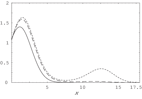
This integral is usually assumed to be dominated by contributions from small values of around the origin , where . The integral is then evaluated numerically either on a grid, or using Monte Carlo simulations. However, for volatilities above the critical value, the integrand develops a second local maximum at large values of the Markov driver as seen in Figure 4, which will dominate the integral above the critical volatility. In the example of Figure 4, the secondary maximum appears at , which is almost 10 standard deviations away from zero. Thus the integral (46) will receive significant contributions from a region in which is sampled very inefficiently in Monte Carlo or grid methods. This implies that the model will not be simulated correctly in the large volatility phase, and the phase transition will be unobservable under these simulation methods.
V Example: constant forward short rate
We illustrate the general results discussed in the previous section on the example of a forward yield curve with constant short rate . The initial yield curve is , and the numeraire rebased discount bonds are .
In Figure 3 we show the zeros of the generating function at the time slice , for a simulation with , total simulation time yr, with time step and time steps. The colored dots show the exact zeros at three values of the volatility around the critical volatility , and the black dots are the zeros of the asymptotic generating function .
We note that the asymptotic generating function gives a reasonably good approximation for the position of the zeros in the large volatility phase. For this reason we discuss in some detail the position of the zeros of the asymptotic generating function for which an analytical treatment is possible in the limit of a constant forward short rate.
The asymptotic generating function for a constant forward short rate is
| (47) |
Its zeros are , where are the zeros of the polynomial of degree
| (48) |
Under usual market conditions , and by the Eneström-Kakeya theorem [10], all zeros of this polynomial lie outside the open unit disk .
The structure of the zeros of can be studied by noting that this polynomial is the truncated Taylor series of the function
| (49) |
The function has an exact zero at , and a pole at , which means that the convergence region is the circle .
The theory of the zeros of a truncated Taylor expansion is a well studied subject in approximation theory. The main result is the Jentzsch-Szegö theorem [11, 12], according to which the zeros of the truncated Taylor series of a function either converge to the zeros of as , provided that they are inside its convergence region, or they accumulate on the boundary of the convergence region. For our case the latter situation applies, such that the zeros of will accumulate uniformly on the circle as the polynomial order increases.
This implies that the zeros of close in on the positive real axis at as the polynomial order becomes large. This phenomenon is visible already at moderate values of , as seen from Fig. 3.
We can compute the properties of the generating function at the critical point by applying the general results discussed above. Taking and , the integral in Eq. (41) can be performed exactly with the result
The jump of the derivative across the critical point is
| (53) |
In the large volatility phase the derivative of is very large, and is of the same order of magnitude as expected from the asymptotic form Eq. (35).
Finally, we consider the case of practical interest of finite polynomial order . It was observed in [13] that for the truncated Taylor series of a function , a good approximation for the moduli of the zeros is obtained by neglecting all but the first and last terms (by considering the simpler polynomial ), provided that the function does not have zeros within the convergence region. In our case of the polynomial , the corresponding polynomial has zeros
| (54) | |||||
The critical volatility can be computed using equation Eq. (39) and is given by
| (55) | |||
The minimum value of is reached at , in the middle of the simulation interval, where is maximal. This agrees with the shape of the curves in Fig. 1, where the critical volatility is first reached in the middle of the interval. Thus the practical applicability range of the model is restricted to volatilities smaller than the minimum critical volatility
| (56) |
This expression satisfies the general scaling properties of the model Eqs. (24).
| 48.95% | 65.10% | 24.48% | 32.55% | 12.24% | 16.28% | 8.16% | 10.85% | |
| 46.04% | 60.70% | 23.02% | 30.35% | 11.51% | 15.17% | 7.67% | 10.12% | |
| 44.24% | 57.96% | 22.12% | 28.98% | 11.06% | 14.49% | 7.37% | 9.66% | |
| 42.92% | 55.94% | 21.46% | 27.97% | 10.73% | 13.99% | 7.15% | 9.32% | |
| 41.87% | 54.32% | 20.93% | 27.16% | 10.47% | 13.58% | 6.98% | 9.05% | |
In Table 1 we show the values of the maximally allowed volatility for several values of the total simulation tenor , the time step , and the short rate . The maximum allowed volatility decreases with the size of the time step , with the tenor of the simulation , and with the short rate .
VI Conclusions
We discussed in this paper the behaviour of a Markov functional model with discrete log-normally distributed Libors, as a function of the Libor volatility. The model can be solved exactly in the forward measure in the limit of a time-independent volatility, by a backwards recursion relation. Analytical results can be obtained for the functional dependence of all discount bonds on the Markov driver.
We showed that the model has two volatility regimes, corresponding to small and large volatility, with very different qualitative behaviour. As the Libor volatility increases, there is a transition between the two regimes, at an intermediate critical volatility. In the large volatility phase the convexity adjusted Libors are very small, and can be below machine precision. Thus the existence of the large volatility regime imposes a limit on the applicability of such a model, which is manifested as an upper bound on the allowed Libor volatility.
We formulated the conditions under which this phase transition occurs, and showed that it is related to the position of the zeros of an appropriately defined generating function in the complex plane. The transition appears for long simulation times, and small time discretization steps. A similar phenomenon is expected to occur also for the practically relevant but analytically more complex case of time-dependent volatility . Also, the discussion of this paper is limited to the forward measure, and one expects that the details of the volatility dependence could change in a different measure, but not the existence of a phase transition. We hope to report progress along these directions in future work.
Appendix A The zeros of the generating function
We study here the distribution of the complex zeros of the asymptotic generating function for a constant forward short rate . This is related to the problem of finding the zeros of the polynomial
| (57) |
where is a real number larger than 1. They are the same as the zeros of the equation from which is excluded. Expressed in polar coordinates one finds that the zeros are on the curve which is given by the solution to the equation
| (58) |
Figure 5 shows the exact roots of , along with the curve (solid line), and the circle with radius (dashed line), which was used in the main text. We note that the latter approximates the moduli of the zeros very well, as noted in [13].

The curve intersects the real axis at some point . The solution of the equation (58) at has always the solution , and in addition it can have another 2 solutions, or none, depending on the values of . The solutions different from 1 can be found as the solutions of the simpler equation . The function has a minimum at . We distinguish the 3 cases, according to the value of
| (59) | |||||
| (60) | |||||
| (61) |
These cases are obtained for respectively, where is the solution of the equation
| (62) |
For one has . A good approximation for the solutions in case 1 is obtained by Taylor expanding around to quadratic order. This gives
| (63) |
In Fig. 5 we show only the largest of the 3 solutions.
The angular distribution of the roots can be obtained from the imaginary part of the equation for , which reads . For the subset of even , this has real solutions for only if is in one of the regions
| (64) |
There is one solution in each of these intervals of equal angular opening, which means that in the large limit, the angular distribution of the roots approaches a uniform distribution . In the same limit, the curve approaches the unit circle , as required by the Jentzsch-Szegö theorem.
Acknowledgements
I am grateful to Dyutiman Das and Adrian Ghinculov for useful discussions on this problem, and to Radu Constantinescu for comments on the manuscript.
References
- [1] P. Hunt, J. Kennedy and A. Pellser, Markov-Functional Interest Rate Models, Finance and Stochastics, 4, 391-408 (2000).
- [2] J. B. Hunt and J. E. Kennedy, Financial Derivatives in Theory and Practice, Wiley Series in Probability and Statistics, 2005.
- [3] P. Balland and L. P. Hughston, Markov Market Model Consistent with Cap Smile, Int. J. Th. Appl. Finance 3, 161-181 (2000).
- [4] P. Glasserman and X. Zhao, Arbitrage free discretization of log-normal forward Libor and swap rate models, Finance and Stochastics 4, 35-68 (2000)
- [5] K. Miltersen, L. Sandmann and D. Sondermann, Closed Form Solutions for Term Structure Derivatives with Log-normal Interest Rates, J. Finance 52, 409-430 (1997).
- [6] L. U. Dothan, On the Term Structure of Interest Rates, Journal of Financial Economics 6, 59-69 (1978).
- [7] D. Brigo and F. Mercurio, Interest Rate Models - Theory and Practice: With Smile, Inflation and Credit, Springer Verlag 2006.
- [8] Eugene H. Stanley, Introduction to Phase Transitions and Critical Phenomena, Oxford University Press, 1987.
- [9] T. D. Lee and C. N. Yang, Statistical Theory of Equations of State and Phase Transitions. II. Lattice Gas and Ising Model, Physical Review Letters 87, 410-419 (1952); Phys. Rev. 87, 410 (1952).
- [10] P. B. Borwein and T. Erdelyi, Polynomials and Polynomial Inequalities, Graduate Texts in Mathematics 161, Springer Verlag, 1995.
- [11] R. Jentzsch, Untersuchungen zur Theorie der Folgen analytischer Funktionen, Acta Math. 41, 219-251 (1918).
- [12] G. Szegö, Über die Nullstellen von Polynomen, die in einem Kreis gleichmassig konvergieren, Sitzungsber. Ber. Math. Ges., 21, 59-64 (1922).
- [13] S. Christiansen, Per A. Madsen, On Truncated Taylor series and the position of their spurious zeros, Applied Numerical Mathematics, 56, 91-104 (2006).