Scheduling Periodic Real-Time Tasks with Heterogeneous Reward Requirements

I-Hong Hou Affiliation: CSL and Department of CS
University of Illinois
Urbana, IL 61801, USA
ihou2@illinois.edu P. R. Kumar Affiliation: CSL and Department of ECE
University of Illinois
Urbana, IL 61801, USA
prkumar@illinois.edu

Abstract

We study the problem of scheduling periodic real-time tasks so as to meet their individual minimum reward requirements. A task generates jobs that can be given arbitrary service times before their deadlines. A task then obtains rewards based on the service times received by its jobs. We show that this model is compatible to the imprecise computation models and the increasing reward with increasing service models. In contrast to previous work on these models, which mainly focus on maximize the total reward in the system, we aim to fulfill different reward requirements by different tasks, which offers better fairness and allows fine-grained tradeoff between tasks. We first derive a necessary and sufficient condition for a system, along with reward requirements of tasks, to be feasible. We also obtain an off-line feasibility optimal scheduling policy. We then studies a sufficient condition for a policy to be feasibility optimal or achieves some approximation bound. This condition can serve as a guideline for designing on-line scheduling policy and we obtains a greedy policy based on it. We prove that the on-line policy is feasibility optimal when all tasks have the same periods and also obtain an approximation bound for the policy under general cases.

⁰⁰footnotetext: This material is based upon work partially supported by USARO under Contract Nos. W911NF-08-1-0238 and W-911-NF-0710287, AFOSR under Contract FA9550-09-0121, and NSF under Contract No. CNS-07-21992. Any opinions, findings, and conclusions or recommendations expressed in this publication are those of the authors and do not necessarily reflect the views of the above agencies.

I Introduction

In classical hard real-time systems, every job needs to be completed before its deadline, or the system suffers from a timing fault. In practice, many applications allow approximate results and partially completed jobs only degrade the overall performance rather than causing a fault. Imprecise computation models [2, 3] and increasing reward with increasing service (IRIS) models [10] have been proposed to deal with such applications. Most work on these models only aims to minimize the total error, or, equivalently, maximize the total reward of the system without any considerations on fairness. However, in many applications, rewards of different tasks are not additive and satisfying individual reward requirements is more important than maximizing total rewards. For example, consider a server that provides video streams to subscribers. Deadline misses will only cause losses on some frames and degrade the video quality, which is usually tolerable as long as such losses happen infrequently. In such an application, a policy that aims to maximize total reward may end up providing perfect video quality for some subscribers while only offering poor quality for others. In contrast, a desirable policy should aim at providing reasonably good quality to all of its subscribers.

In this paper, we describe a model that considers the hard delay bounds of tasks as well as rewards for partially completed jobs, in a system with a set of periodic tasks. The relationship between service times and rewards can be any arbitrary increasing and concave function and may differ from task to task. We allow each task to have its own individual requirement on the average reward it obtains. We show that both the imprecise computation model and the IRIS model are special cases of our model.

Based on the model, we first analyze the conditions for feasibility, that is, whether there exists a scheduling policy that meets the individual reward requirements of all tasks in the system. We prove a necessary and sufficient condition for feasibility. We also propose a linear time algorithm for evaluating whether a system is feasible. Along with the feasibility condition, we also derive an off-line scheduling policy that is feasibility optimal, meaning that it fulfills all feasible systems.

We then study the problem of designing on-line scheduling policies. We derive a sufficient condition for a policy to be feasibility optimal, or, serve as an approximation policy with some approximation bound. Using this condition as a guideline, we propose an on-line scheduling policy. We prove that this on-line policy fulfills every feasible system in which periods are the same for all tasks. We also obtain an approximation bound for this policy when periods of tasks may be different.

In addition to theoretical studies, we also conduct simulations to verify our results. We compare our policy against one proposed by Aydin et al [1], which is proved to be an optimal off-line policy that maximizes the total reward in any system. Simulation results suggest that although the policy proposed by [1] achieves maximum total reward, it can result in severe unfairness and does not allow fine-grained tradeoffs between the performances of different tasks.

The rest of the paper is organized as follows. Section II summaries some existing work and, in particular, introduces the basic concepts in the imprecise computation model and the IRIS model. Section III formally describes our proposed model and discusses how it can capture the imprecise computation model and the IRIS model. Section IV analyzes the necessary and sufficient condition for a system to be feasible, and proposes a linear time algorithm for evaluating feasibility. Section V studies the problem of scheduling jobs and obtains a sufficient condition for a policy to achieve an approximation bound or to be feasibility optimal. Based on this condition, Section VI proposes a simple on-line scheduling policy and analyzes its performance under different cases. Section VII demonstrates our simulation results. Finally, Section VIII concludes this paper.

II Related Work

The imprecise computation models [2, 3] have been proposed to handle applications in which partially completed jobs are useful. In this model, all jobs consist of two parts: a mandatory part and an optional part. The mandatory part needs to be completed before its deadline, or else the system suffers from a timing fault. On the other hand, the optional part is used to further enhance performance by either reducing errors or increasing rewards. The relations between the errors, or rewards, and the time spent on the optional parts, are described through error functions or reward functions. Chung, Liu, and Lin [2] have proposed scheduling policies that aim to minimize the total average error in the system for this model. Their result is optimal only when the error functions are linear and tasks generate jobs with the same period. Shih and Liu [4] have proposed policies that minimize the maximum error among all tasks in the system when error functions are linear. Feiler and Walker [5] have used feedback to opportunistically schedule optional parts when the lengths of mandatory parts may be time-varying. Mejia-Alvarez, Melhem, and Mosse [6] have studied the problem of maximizing total rewards in the system when job generations are dynamic. Chen et al [7] have proposed scheduling policies that defer optional parts so as to provide more timely response for mandatory parts. Zu and Chang [8] have studied the scheduling problem when optional parts are hierarchical. Aydin et al [1] have proposed an off-line scheduling policy that maximizes total rewards when the reward functions are increasing and concave. Most of these works only concern the maximization of the total reward in a system. Amirijoo, Hansson, and Son [9] have considered the tradeoff between data errors and transaction errors in a real-time database. The IRIS models can be thought of as special cases of the imprecise computation models where the lengths of mandatory parts are zero. Scheduling policies aimed at maximizing total rewards have been studied for such models [10, 11].

III System Model

Consider a system with a set $S=\{A,B,\dots\}$ of real-time tasks. Time is slotted and expressed by $t\in\{0,1,2,\dots\}$ . Each task $X$ generates a job periodically with period $\tau_{X}$ . A job can be executed multiple times in the period that it is generated; the execution of a job does not mean its completion. The job is removed from the system when the next period begins. In other words, the relative deadline of a job generated by task $X$ is also $\tau_{X}$ . We assume that all tasks in $S$ generate a job at time $t=0$ . We denote a frame as the time between two consecutive time slots where all tasks generate a job. The length of a frame, which we denote by $T$ , is the least common multiple of $\{\tau_{X}|X\in S\}$ . Thus, a frame consists of $T/\tau_{X}$ periods of task $X$ .

As noted above, each job can be executed an arbitrary number of time slots before its deadline. Each task obtains a certain reward each time that its job is executed. The total amount of reward obtained by a task in a period depends on the number of times that its job has been executed in the period. More formally, task $X$ obtains reward $r^{i}_{X}\geq 0$ when it executes its job for the $i^{th}$ time in a period. For example, if a job of task $X$ is executed a total of $n$ time slots, then the total reward obtained by task $X$ in this period is $r^{1}_{X}+r^{2}_{X}+\dots+r^{n}_{X}$ . We further assume that the marginal reward of executing a job decreases as the number of executions increases, that is, $r^{i+1}_{X}\leq r^{i}_{X}$ , for all $i$ and $X$ . Thus, the total reward that a task obtains in a period is an increasing and concave function of the number of time slots that its job is executed.

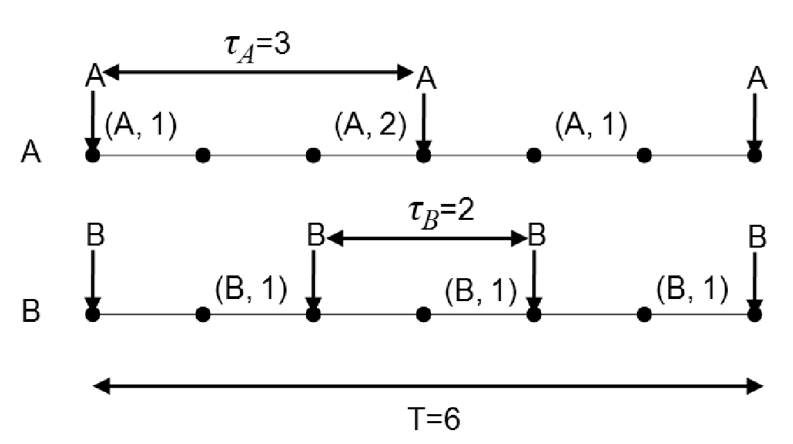
A scheduling policy $\eta$ for the system is one that chooses an action in each time slot. The action taken by $\eta$ at time $t$ is described by $\eta(t)=(X,i)$ , meaning that the policy executes the job of task $X$ at time $t$ and that this is the $i^{th}$ time that the job is being executed in the period. Fig. 1 shows an example with two tasks over one frame, which consists of two periods of task $A$ and three periods of task $B$ . In this example, action $(A,1)$ is executed twice and $(A,2)$ is executed once. Thus, the reward obtained by task $A$ in this frame is $2r^{1}_{A}+r^{2}_{A}$ . On the other hand, the reward obtained by task $B$ in this frame is $3r^{1}_{B}$ .

Refer to caption — Fig. 1: An example of the system and scheduling policy over a frame of six slots, which consists of two period of task $A$ and three periods of task $B$ . Arrows in the figure indicate the beginning of a new period.

The performance of the system is described by the long-term average reward per frame of each task in the system.

Definition 1

Let $s_{X}(t)$ be the total reward obtained by task $X$ between time 0 and time $t$ under some scheduling policy $\eta$ . The average reward of task $X$ is defined as $q_{X}:=\liminf_{t\rightarrow\infty}\frac{s_{X}(t)}{t/T}$ .

We assume that there is a minimum average reward requirement for each task $X$ , $q^{*}_{X}>0$ . We wish to verify whether a system is feasible, that is, whether each task can have its minimum average reward requirement satisfied.

Definition 2

A system is fulfilled by a scheduling policy $\eta$ if, under $\eta$ , $q_{X}\geq q^{*}_{X}$ with probability 1, for all $X\in S$ .

Definition 3

A system is feasible if there exists some scheduling policy that fulfills it.

A natural metric to evaluate a scheduling policy is the set of systems that the policy fulfills. For ease of discussion, we only consider systems that are strictly feasible

Definition 4

A system with minimum reward requirements $[q^{*}_{X}|X\in S]$ is strictly feasible if there exists some $\epsilon>0$ such that the same system with minimum reward requirements $[(1+\epsilon)q^{*}_{X}]$ is feasible.

Definition 5

A scheduling policy is feasibility optimal if it fulfills all strictly feasible systems.

Moreover, since the overhead for computing a feasibility optimal policy may be too high in certain scenarios, we also need to consider simple approximation policies.

Definition 6

A scheduling policy is a $p$ -approximation policy, $p\geq 1$ , if it fulfills all systems with minimum reward requirements $[q^{*}_{X}]$ such that the same system with minimum reward requirements $[pq^{*}_{X}]$ is strictly feasible.

III-A Extensions for Imprecise Computation Models

In this section, we discuss how our proposed model can be used to handle imprecise computation models and IRIS models. In such models, a task consists of two parts: a mandatory part and an optional part. The mandatory part is required to be completed in each period, or else the system fails. After the mandatory part is completed, the optional part can be executed to improve performance. The more optional parts executed for a task, the more rewards it gets.

Let $m_{X}$ be the length of the mandatory part of task $X$ , that is, it is required that each job of $X$ is executed at least $m_{X}$ time slots in each of its period. Let $o_{X}$ be the length of the optional part of task $X$ . To accommodate this scenario, we define a symbolic value $M$ with the following arithmetic reminiscent of the “Big- $M$ Method” in linear programming: $0\times M=0$ , $aM+bM=(a+b)M$ , $a\times(bM)=(ab)M$ , $aM+c>bM+d$ , if $a>b$ , and $aM+c>aM+d$ if $c>d$ , for all real numbers $a,b,c,d$ . Loosely speaking, $M$ can be thought of as a huge positive number. For each task $X$ , we set $r^{1}_{X}=r^{2}_{X}=\dots=r^{m_{X}}_{X}=M$ , we then set $r^{m_{X}+1}_{X},r^{m_{X}+2}_{X},\dots,r^{m_{X}+o_{X}}_{X}$ according to the rewards obtained by $X$ for its optional part, and $r^{i}_{X}=0$ , for all $i>m_{X}+o_{X}$ . The minimum reward requirement of task $X$ is set to be $\frac{T}{\tau_{X}}m_{X}M+\hat{q}^{*}_{X}$ with $\hat{q}^{*}_{X}\geq 0$ . Thus, a scheduling policy that fulfills such a system is guaranteed to complete each mandatory part with probability one.

IV Feasibility Analysis

In this section, we establish a necessary and sufficient condition for a system to be feasible. Consider a feasible system that is fulfilled by a policy $\eta$ . Suppose that, on average, there are $f^{i}_{X}$ periods of task $X$ in a frame in which the action $(X,i)$ is taken by $\eta$ . The average reward of task $X$ can then be expressed as $q_{X}=\sum_{i=1}^{\tau_{X}}f^{i}_{X}r^{i}_{X}$ . We can immediately obtain a necessary condition for feasibility.

Lemma 1

A system with a set of tasks $S=\{A,B,\dots\}$ is feasible only if there exists $\{f^{i}_{X}|X\in S,1\leq i\leq\tau_{X}\}$ such that

$\displaystyle q^{*}_{X}\leq\sum_{i=1}^{\tau_{X}}f^{i}_{X}r^{i}_{X},$	$\displaystyle\forall X\in S,$	(1)
$\displaystyle 0\leq f^{i}_{X}\leq\frac{T}{\tau_{X}},$	$\displaystyle\forall X\in S,1\leq i\leq\tau_{X},$	(2)
$\displaystyle\sum_{X\in S}\sum_{i=1}^{\tau_{X}}f^{i}_{X}\leq T.$		(3)

Proof:

Condition (1) holds because task $X$ requires that $q^{*}_{X}\leq q_{X}$ . Condition (2) holds because there are $T/\tau_{X}$ periods of task $X$ in a frame and thus $f^{i}_{X}$ is upper-bounded by $T/\tau_{X}$ . Finally, the total average number of time slots that the system executes one of the jobs in a frame can be expressed as $\sum_{X\in S}\sum_{i=1}^{\tau_{X}}f^{i}_{X}$ , which is upper-bounded by the number of time slots in a frame, $T$ . Thus, condition (3) follows. ∎

Next, we show that the conditions (1)–(3) are also sufficient for feasibility. To prove this, we first show that the polytope, which contains all points $f=(f^{1}_{A},f^{2}_{A},\dots,f^{\tau_{A}}_{A},f^{1}_{B},\dots)$ that satisfy conditions (2) and (3), is a convex hull of several integer points. We then show that for all integer points $n=(n^{1}_{A},n^{2}_{A},\dots,n^{\tau_{A}}_{A},n^{1}_{B},\dots)$ in the polytope, there is a schedule under which the reward obtained by task $X$ is at least $\sum_{i=1}^{\tau_{X}}n^{i}_{X}r^{i}_{X}$ . We then prove sufficiency using these two results.

Define a matrix $H=[h_{i,j}]$ with $2\sum_{X\in S}\tau_{X}+1$ rows and $\sum_{X\in S}\tau_{X}$ columns as follows:

h_{i,j}=\left\{\begin{array}[]{rl}1,&\mbox{if $i=1$,}\\ 1,&\mbox{if $i=2j$,}\\ -1,&\mbox{if $i=2j+1$,}\\ 0,&\mbox{else.}\end{array}\right.

(4)

Define $b=[b_{i}]$ to be a column vector with $2\sum_{X\in S}\tau_{X}+1$ elements so that $b_{1}=T$ ; the first $\tau_{A}$ elements with even indices are set to $T/\tau_{A}$ , that is, $b_{2}=b_{4}=\dots=b_{2\tau_{A}}=T/\tau_{A}$ ; the next $\tau_{B}$ elements with even indices are set to $T/\tau_{B}$ , and so on. All other elements are set to 0. For example, the system shown in Fig. 1 would have

H=\left[\begin{array}[]{rrrrr}1,&1,&1,&1,&\dots\\ 1,&0,&0,&0,&\dots\\ -1,&0,&0,&0,&\dots\\ 0,&1,&0,&0,&\dots\\ 0,&-1,&0,&0,&\dots\\ 0,&0,&1,&0,&\dots\\ 0,&0,&-1,&0,&\dots\\ &&\vdots\end{array}\right],b=\left[\begin{array}[]{c}T\\ T/\tau_{A}\\ 0\\ T/\tau_{A}\\ 0\\ \vdots\\ T/\tau_{B}\\ 0\\ \vdots\end{array}\right].

Thus, conditions (2) and (3) can be described as $Hf\leq b$ . Theorem 5.20 and Theorem 5.24 in [12] shows the following:

Theorem 1

The polytope defined by $\{f|Hf\leq b\}$ , where $b$ is an integer vector, is a convex hull of several integer points if for every subset $R$ of rows in $H$ , there exists a partition of $R=R_{1}\cup R_{2}$ such that for every column $j$ in $H$ , we have $\sum_{i_{1}\in R_{1}}h_{i_{1},j}-\sum_{i_{2}\in R_{2}}h_{i_{2},j}\in\{1,0,-1\}$ .¹¹ 1 Such matrix $H$ is called a totally unimodular matrix in combinatorial optimization theory.

Since all elements in $b$ are integers, we obtain the following:

Theorem 2

The polytope defined by $\{f|Hf\leq b\}$ , where $H$ and $b$ are derived using conditions (2) and (3) as above, is a convex hull of several integer points.

Proof:

Let $R=\{r_{1},r_{2},\dots\}$ be the indices of some subset of rows in $H$ . If the first row is in $R$ , we choose $R_{1}=\{r|r\in R,\mbox{$r$ is odd}\}$ and $R_{2}=\{r|r\in R,\mbox{$r$ is even}\}$ . Since for all columns $j$ in $H$ , $h_{1,j}=1$ , $h_{2j,j}=1$ , $h_{2j+1,j}=-1$ , and all other elements in column $j$ are zero, we have $\sum_{i_{1}\in R_{1}}h_{i_{1},j}-\sum_{i_{2}\in R_{2}}h_{i_{2},j}\in\{1,0,-1\}$ . On the other hand, if the first row is not in $R$ , we choose $R_{1}=R$ and $R_{2}=\varnothing$ . Again, we have $\sum_{i_{1}\in R_{1}}h_{i_{1},j}-\sum_{i_{2}\in R_{2}}h_{i_{2},j}=\sum_{i_{1}\in R_{1}}h_{i_{1},j}\in\{1,0,-1\}$ . Thus, by Theorem 1, the polytope defined by $\{f|Hf\leq b\}$ is a convex hull of several integer points. ∎

Next we show that all integer points in the polytope can be carried out by some scheduling policy as follows:

Theorem 3

Let $n=(n^{1}_{A},n^{2}_{A},\dots,n^{\tau_{A}}_{A},n^{1}_{B},\dots)$ be an integer point in the polytope $\{f|Hf\leq b\}$ . Then, there exists a scheduling policy so that $q_{X}\geq\sum_{i=1}^{\tau_{X}}n^{i}_{X}r^{i}_{X}$ .

Proof:

We prove this theorem by constructing a scheduling policy that achieves the aforementioned requirement. We begin by marking deadlines of actions. Ideally, we wish to schedule the action $(X,i)$ $n^{i}_{X}$ times in a frame. Without loss of generality, we assume that the frame starts at time $0$ and ends at time $T$ . Since there is at most one $(X,i)$ action in a period of task $X$ , we can mark the deadlines of these actions as $T,T-\tau_{X},\dots,T-(n^{i}_{X}-1)\tau_{X}$ , respectively. The scheduling policy will schedule the action with the earliest deadline that has neither been executed in its period (that is, it does not schedule two actions of the same type in the same period) nor missed its deadline, with ties broken arbitrarily. Fig. 2a shows how the deadlines are marked in an example with $n^{1}_{A}=1,n^{2}_{A}=2,n^{1}_{B}=2,$ and $n^{2}_{B}=1$ . Fig. 2b shows the resulting schedule for this example. Note that, under this policy, there are time slots where the policy schedules an action $(X,i)$ , but it is instead the $j^{th}$ time that the job of $X$ is executed in the period. Thus, we may need to renumber these actions as in Fig. 2c and define $\bar{n}^{i}_{X}$ as the actual number of times that the action $(X,i)$ is executed in the frame. In the example of Fig. 2, we have $\bar{n}^{1}_{A}=2,\bar{n}^{2}_{A}=1,\bar{n}^{1}_{B}=3$ , and $\bar{n}^{2}_{B}=0$ . Since the policy does not schedule two identical actions in a period, as long as all actions are executed before their respective deadlines, we have $\sum_{i=1}^{k}\bar{n}^{i}_{X}\geq\sum_{i=1}^{k}n^{i}_{X}$ , for all $k$ and $X\in S$ . Thus, $q_{X}=\sum_{i=1}^{\tau_{X}}\bar{n}^{i}_{X}r^{i}_{X}\geq\sum_{i=1}^{\tau_{X}}n^{i}_{X}r^{i}_{X}$ , since $r^{1}_{X}\geq r^{2}_{X}\geq\dots$ , for all $X\in S$ . To avoid confusion, we refer actions by its type before renumbering throughout the rest of the proof.

It remains to show that none of the actions miss their deadlines under this policy. We prove this by contradiction. Let $d_{X}(t)$ be the number of actions of task $X$ whose deadlines are smaller or equal to $t$ . By the way that we mark deadlines of actions, we have that $\frac{d_{X}(\tau_{X})}{\tau_{X}}\leq\frac{d_{X}(2\tau_{X})}{2\tau_{X}}\leq\dots\leq\frac{d_{X}(T)}{T}$ . We also have $d_{X}(t)=d_{X}(k\tau_{X})$ , for all $t\in[k\tau_{X},(k+1)\tau_{X})$ . For any $t$ , let $k_{X}=\lfloor\frac{t}{\tau_{X}}\rfloor$ , and we then have

\begin{array}[]{rl}\sum_{X\in S}\frac{d_{X}(t)}{t}&=\sum_{X\in S}\frac{d_{X}(k_{X}\tau_{X})}{t}\\ &\leq\sum_{X\in S}\frac{d_{X}(k_{X}\tau_{X})}{k_{X}\tau_{X}}\\ &\leq\frac{\sum_{X\in S}d_{X}(T)}{T}\leq 1,\end{array}

(5)

where the last inequality follows by condition (3).

Suppose there is an action $(X,i)$ that misses its deadline at time $t$ under our policy. We first consider the case where the policy schedules an action with deadline smaller or equal to $t$ in all time slots between 0 and $t$ , with no time slot left idle. In this case, we have $\sum_{X\in S}d_{X}(t)\geq t+1$ and thus $\sum_{X\in S}\frac{d_{X}(t)}{t}>1$ , which contradicts Eq. (5).

Next we consider the case where at some time $t^{\prime}<t$ the policy does not schedule an action with deadline smaller or equal to $t$ . That is, at time $t^{\prime}$ , the policy either schedules an action whose deadline is strictly larger than $t$ or stays idle. Now we first claim that $t$ and $t^{\prime}$ cannot belong to the same period of $X$ , that is, the case with $t^{\prime}>t-\tau_{X}$ is not possible. The only reason that $(X,i)$ is not in fact scheduled at $t^{\prime}$ is that there is already one identical action in the corresponding period containing $t^{\prime}$ . This other action would have a deadline at either $t$ or $t-k\tau_{X}$ for some $k\geq 1$ . The former case is not possible because two identical actions cannot have the same deadline. The latter is also not possible because no action is scheduled after its deadline and $t-k\tau_{X}<t^{\prime}$ if $t$ and $t^{\prime}$ belong to the same period.

As shown above, the interval $[t-\tau_{X}+1,t]$ has the property that all actions scheduled in this interval have deadlines smaller or equal to $t$ . Now we proceed to show that $t^{\prime}\leq t-\tau_{X}$ is also not possible. We do this by expanding this interval while preserving this property. Pick any action, $(X^{\prime},i^{\prime})$ , scheduled at time $t_{X^{\prime}}$ in the interval and assume that the period of $X^{\prime}$ containing $t_{X^{\prime}}$ is $[t^{1}_{X^{\prime}},t^{2}_{X^{\prime}}]$ . We have $t^{2}_{X^{\prime}}\leq t$ since the deadline of $({X^{\prime}},i^{\prime})$ is no larger than $t$ and the deadline of this action is at the end of some period of $X^{\prime}$ . Now, by the design of the scheduling policy, for any $\bar{t}_{X^{\prime}}$ in $[t^{1}_{X^{\prime}},t_{X^{\prime}}]$ , the action scheduled in $\bar{t}_{X^{\prime}}$ should have deadline smaller or equal to the deadline of $({X^{\prime}},i^{\prime})$ , or otherwise $({X^{\prime}},i^{\prime})$ should have been scheduled in $\bar{t}_{X^{\prime}}$ . The deadline of the action scheduled in $\bar{t}_{X^{\prime}}$ is thus also smaller or equal to $t$ . Thus, if $t^{1}_{X^{\prime}}$ is smaller than the beginning of the interval, we can expand the interval to $[t^{1}_{X^{\prime}},t]$ while preserving the desired property. We keep expanding the interval until no more expansions are possible.

Let $(Y,j)$ be the action in the resulting interval with the largest period, $\tau_{Y}$ , and suppose that it is scheduled at time $t_{Y}$ . Assume that the period of $Y$ containing $t_{Y}$ is $[t^{1}_{Y},t^{2}_{Y}]$ . By the way we expand the interval, $[t^{1}_{Y},t^{2}_{Y}]$ is within the expanded interval and all actions scheduled in $[t^{1}_{Y},t^{2}_{Y}]$ have deadlines smaller or equal to $t$ . For each action in $[t^{1}_{Y},t^{2}_{Y}]$ , the reason that it has not been scheduled earlier at time $t^{\prime}$ is because there is already one identical action scheduled in its period that contains $t^{\prime}$ . This identical action, also with deadline earlier than $t$ , must have been scheduled before time $t^{\prime}$ . Since the period of this action is smaller or equal to $\tau_{Y}$ , its identical counterpart must have been scheduled in $[t^{\prime}-\tau_{Y}+1,t^{\prime}-1]$ . However, there are at most $\tau_{Y}-1$ actions scheduled in $[t^{\prime}-\tau_{Y}+1,t^{\prime}-1]$ , while there are $\tau_{Y}$ actions in $[t^{1}_{Y},t^{2}_{Y}]$ , leading to a contradiction. Thus, this case is also not possible.

In sum, all actions are scheduled before their deadlines using this policy, and the proof is completed. ∎

Now we can derive the necessary and sufficient condition for a system to be feasible.

Theorem 4

A system with a set of tasks $S=\{A,B,\dots\}$ is feasible if and only if there exists $\{f^{i}_{X}|X\in S,1\leq i\leq\tau_{X}\}$ such that (1) - (3) are satisfied.

Proof:

Lemma 1 has established that these conditions are necessary. It remains to show that they are also sufficient. Suppose there exists $f=\{f^{i}_{X}|X\in S,1\leq i\leq\tau_{X}\}$ that satisfy (1) - (3), then Theorem 2 shows that there exists integer vectors $n[1],n[2],\dots,n[v]$ such that $f=\sum_{u=1}^{v}\alpha_{u}n[u]$ , where $\alpha_{u}$ ’s are positive numbers with $\sum_{u=1}^{v}\alpha_{u}=1$ . Let $\eta_{u}$ be the scheduling policy for the integer vector $n[u]$ as in the proof of Theorem 3, for each $u$ . Theorem 3 have shown that for each $u$ , the average reward obtained by $X$ under $\eta_{u}$ , $q_{X}[\eta_{u}]$ , is at least $\sum_{i=1}^{\tau_{X}}n[u]^{i}_{X}r^{i}_{X}$ . Finally, we can design a policy as a weighted round robin policy that switches among the policies $\eta_{1},\eta_{2},\dots,\eta_{v}$ , with policy $\eta_{u}$ being chosen in $\alpha_{u}$ of the frames. The average reward obtained by $X$ is hence $q_{X}=\sum_{u}\alpha_{u}q_{X}[\eta_{u}]\geq\sum_{u}\alpha_{u}(\sum_{i=1}^{\tau_{X}}n[u]^{i}_{X}r^{i}_{X})=\sum_{i=1}^{\tau_{X}}f^{i}_{X}r^{i}_{X}\geq q^{*}_{X}$ . Thus, this policy fulfills the system and so the conditions are also sufficient. ∎

Using Theorem 4, checking whether a system is feasible can be done by any linear programming solver. The computational overhead for checking feasibility can be further reduced by using the fact that $r^{i}_{X}\geq r^{j}_{X}$ , for all $i<j$ . Given a system and $\{f^{i}_{X}\}$ that satisfies conditions (1) - (3) with $f^{j}_{Y}<\frac{T}{\tau_{Y}}$ and $f^{k}_{Y}>0$ for some $j<k$ and $Y\in S$ . Let $\delta=\min\{\frac{T}{\tau_{Y}}-f^{j}_{Y},f^{k}_{Y}\}$ . Construct $\{\hat{f}^{i}_{X}\}$ such that $\hat{f}^{j}_{Y}=f^{j}_{Y}+\delta$ , $\hat{f}^{k}_{Y}=f^{k}_{Y}-\delta$ , and $\hat{f}^{i}_{X}=f^{i}_{X}$ for all other elements. Then $\{\hat{f}^{i}_{X}\}$ also satisfies conditions (1) - (3). Based on this observation, we derive an algorithm for checking feasibility as shown in Algorithm 1. This essentially transfers slots from less reward earning actions to more reward earning actions. The running time of this algorithm is $O(\sum_{X\in S}\tau_{X})$ . Since a specification of a system involves at least the $\sum_{X\in S}\tau_{X}$ variables of $\{r^{i}_{X}\}$ , Algorithm 1 is essentially a linear time algorithm.

Algorithm 1 Feasibility Checker

S

\{\tau_{X}|X\in S\}

\{r^{i}_{X}|X\in S,1\leq i\leq\tau_{X}\}

\{q^{*}_{X}|X\in S\}

1: for

X\in S

2: if

q^{*}_{X}>\frac{T}{\tau_{X}}\sum_{i=1}^{\tau_{X}}r^{i}_{X}

then

3: return Infeasible

4: end if

5: end for

6: for

X\in S

i\leftarrow 1

8: while

q^{*}_{X}>0

9: if

q^{*}_{X}>\frac{T}{\tau_{X}}r^{i}_{X}

then

10:

f^{i}_{X}\leftarrow T/\tau_{X}

11:

q^{*}_{X}\leftarrow q^{*}_{X}-\frac{T}{\tau_{X}}r^{i}_{X}

12: else

13:

f^{i}_{X}\leftarrow q^{*}_{X}/r^{i}_{X}

14:

q^{*}_{X}\leftarrow 0

15: end if

16:

i\leftarrow i+1

17: end while

18: end for

19: if

\sum_{X\in S}\sum^{i=1}_{\tau_{X}}f^{i}_{X}\leq T

then

20: return Feasible

21: else

22: return Infeasible

23: end if

In addition to evaluating feasibility, the proof of Theorem 4 also demonstrates an off-line feasibility optimal policy. In many scenarios, however, on-line policies are preferred. In the next section, we introduce a guideline for designing scheduling policies that turns out to suggest simple on-line policies.

V Designing Scheduling Policies

In this section, we study the problem of designing scheduling policies. We establish sufficient conditions for a policy to be either feasibility optimal or $p$ -approximately so.

We start by introducing a metric to evaluate the performance of a policy $\eta$ . Let $\tilde{q}_{X}(k)$ be the total reward obtained by task $X$ during the frame $((k-1)T,kT]$ . We then have $q_{X}=\liminf_{k\rightarrow\infty}\frac{\sum_{i=1}^{k}\tilde{q}_{X}(i)}{k}$ . We also define the debt of task $X$ .

Definition 7

The debt of task $X$ in the frame $((k-1)T,kT]$ , $d_{X}(k)$ is defined recursively as follows:

		$\displaystyle d_{X}(0)=0,$
		$\displaystyle d_{X}(k)=[d_{X}(k-1)+q^{*}_{X}-\tilde{q}_{X}(k)]^{+},\forall k>0.$

Lemma 2

A system is fulfilled by a policy $\eta$ if $\lim_{k\rightarrow\infty}d_{X}(k)/k=0$ with probability 1.

Proof:

We have $d_{X}(k)\geq kq^{*}_{X}-\sum_{i=1}^{k}\tilde{q}_{X}(i)$ and $d_{X}(k)/k\geq q^{*}_{X}-\frac{1}{k}\sum_{i=1}^{k}\tilde{q}_{X}(i)$ . Thus, if $\lim_{k\rightarrow\infty}d_{X}(k)/k=0$ , then $q_{X}=\liminf_{k\rightarrow\infty}\frac{\sum_{i=1}^{k}\tilde{q}_{X}(i)}{k}\geq q^{*}_{X}$ and the system is fulfilled. ∎

We can describe the state of the system in the $k^{th}$ frame by the debts of tasks, $[d_{X}(k)|X\in S]$ . Consider a policy that schedules jobs solely based on the requirements and the state of the system. The evolution of the state of the system can then be described as a Markov chain.

Lemma 3

Suppose the evolution of the state of a system can be described as a Markov chain under some policy $\eta$ . The system is fulfilled by $\eta$ if this Markov chain is irreducible and positive recurrent.

Proof:

Since the Markov chain is positive recurrent, the state $\{d_{X}(k)=0,\forall X\in S\}$ is visited infinitely many times. Further, assuming that the system is in this state at frames $k_{1},k_{2},k_{3},\dots$ , then $[k_{n+1}-k_{n}]$ is a series of i.i.d. random variables with finite mean. Let $I_{n}$ be the indicator variable that there exists some $\tilde{k}_{n}$ between frame $k_{n}$ and frame $k_{n+1}$ such that $d_{X}(\tilde{k}_{n})/\tilde{k}_{n}>\delta$ for some $X\in S$ , for some arbitrary $\delta>0$ . Let $q^{*}_{max}=\max_{X\in S}{q^{*}_{X}}$ . If $I_{n}=1$ , we have that $\tilde{k}_{n}\geq k_{n}\geq n$ and thus $d_{X}(\tilde{k}_{n})>n\delta$ , for some $X\in S$ . Since $d_{X}(k)$ can be incremented by at most $q^{*}_{max}$ in a frame and $d_{X}(k_{n})=0$ , $\tilde{k}_{n}-k_{n}>n\delta/q^{*}_{max}$ and $k_{n+1}-k_{n}>\tilde{k}_{n}-k_{n}>n\delta/q^{*}_{max}$ . Thus,

	$\displaystyle Prob\{I_{n}=1\}$	$\displaystyle<Prob\{k_{n+1}-k_{n}>n\delta/q^{*}_{max}\}$
		$\displaystyle=Prob\{k_{2}-k_{1}>n\delta/q^{*}_{max}\},$

and

	$\displaystyle\sum_{n=1}^{\infty}Prob\{I_{n}=1\}$	$\displaystyle<\sum_{n=1}^{\infty}Prob\{k_{2}-k_{1}>n\delta/q^{*}_{max}\}$
		$\displaystyle\leq E[k_{2}-k_{1}]<\infty,$

By Borel-Cantelli Lemma, the probability that $I_{n}=1$ for infinitely many $n$ ’s is zero, and so is the probability that $d_{X}(k)/k>\delta$ for infinitely many $k$ ’s. Thus, $\limsup_{k\rightarrow\infty}d_{X}(k)/k<\delta$ with probability 1, for all $X\in S$ and any arbitrary $\delta>0$ . Finally, we have $\lim_{k\rightarrow\infty}d_{X}(k)/k=0$ with probability 1 since $d_{X}(k)\geq 0$ by definition. ∎

Based on the above lemmas, we determine a sufficient condition for a policy to be a $p$ -approximation policy. The proof is based on the Foster-Lyapunov Theorem:

Theorem 5 (Foster-Lyapunov Theorem)

Consider a Markov chain with state space $\mathcal{D}$ . Let $D(k)$ be the state of the Markov chain at the $k^{th}$ step. If there exists a non-negative function $L:\mathcal{D}\rightarrow R$ , a positive number $\delta$ , and a finite subset $\mathcal{D}_{0}$ of $\mathcal{D}$ such that:

	$\displaystyle E[L(D(k+1))-L(D(k))\|D(k)]\leq-\delta,$	$\displaystyle\mbox{ if $D(k)\notin\mathcal{D}_{0}$},$
	$\displaystyle E[L(D(k+1))\|D(k)]<\infty,$	$\displaystyle\mbox{ if $D(k)\in\mathcal{D}_{0}$},$

then the Markov chain is positive recurrent. $\blacksquare$

Theorem 6

A policy $\eta$ is a $p$ -approximation policy, for some $p>1$ , if it schedules jobs solely based on the requirements and the state of a system and, for each $k$ , the following holds:

\sum_{X\in S}\tilde{q}_{X}(k)d_{X}(k)\geq(\max_{\mbox{$[q_{X}]$: $[q_{X}]$ is feasible}}\sum_{X\in S}q_{X}d_{X}(k))/p.

Proof:

Consider a system with minimum reward requirements $[q^{*}_{X}]$ such that the same system with minimum reward requirements $[pq^{*}_{X}]$ is also strictly feasible. By Lemma 3, it suffices to show that under the policy $\eta$ , the resulting Markov chain is positive recurrent. Consider the Lyapunov function $L(k):=\sum_{X\in S}d^{2}_{X}(k)/2$ . The Lyapunov drift function can be written as:

	$\displaystyle\Delta L(k+1):=$	$\displaystyle L(k+1)-L(k)=\frac{1}{2}\sum_{X\in S}[d^{2}_{X}(k+1)-d^{2}_{X}(k)]$
	$\displaystyle\leq$	$\displaystyle\sum_{X\in S}(q^{*}_{X}-\tilde{q}_{X}(k))d_{X}(k)+C,$

where $C$ is a bounded constant. Since $[pq^{*}_{X}]$ is also strictly feasible and $d_{X}(k)\geq 0$ , there exists $\epsilon>0$ such that $(1+\epsilon)\sum_{X\in S}pq^{*}_{X}d_{X}(k)\leq\max_{\mbox{$[q_{X}]$: $[q_{X}]$ is feasible}}\sum_{X\in S}q_{X}d_{X}(k)$ , and hence $(1+\epsilon)\sum_{X\in S}q^{*}_{X}d_{X}(k)\leq\sum_{X\in S}\tilde{q}_{X}(k)d_{X}(k)$ . Thus, we have

\Delta L(k+1)\leq-\epsilon\sum_{X\in S}q^{*}_{X}d_{X}(k)+C.

(6)

Let $\mathcal{D}_{0}$ be the set of states $[d_{X}(k)|X\in S]$ with $\sum_{X\in S}q^{*}_{X}d_{X}(k)<(C+\delta)/\epsilon$ , for some positive finite number $\delta$ . Then, $\mathcal{D}_{0}$ is a finite set (since $q^{*}_{X}>0$ for all $x\in S$ ), with $\Delta L(k+1)<-\delta$ when the state of frame $k$ is not in $\mathcal{D}_{0}$ . Further, since $d_{X}(k)$ can be increased by at most $q^{*}_{X}$ in each frame, $L(k+1)$ is finite if the state of frame $k$ is in $\mathcal{D}_{0}$ . By Theorem 5, this Markov chain is positive recurrent and policy $\eta$ fulfills this system. ∎

Since a $1$ -approximation policy is also a feasibility optimal one, a similar proof yields the following:

Theorem 7

A policy $\eta$ fulfills a strictly feasible system if it maximizes $\sum_{X\in S}\tilde{q}_{X}(k)d_{X}(k)$ among all feasible $[q_{X}]$ in every frame $k$ . It is a feasibility optimal policy if the above holds for all strictly feasible systems.

VI An On-Line Scheduling Policy

While Section V has described a sufficient condition for designing feasibility optimal policies, the overhead for computing such a feasibility optimal scheduling policy may be too high to implement. In this section, we introduce a simple on-line policy. We also analyze the performance of this policy under different scenarios.

Theorem 7 has shown that a policy that maximizes $\sum_{X\in S}\tilde{q}_{X}(k)d_{X}(k)$ among all feasible $[q_{X}]$ in every frame $k$ is feasibility optimal. The on-line policy follows this guideline by greedily selecting the job with the highest $r^{i}_{x}d_{X}(k)$ in each time slot. Assume that, at some time $t$ in frame $k$ , task $X$ has already been scheduled $i_{X}$ times in its period. The on-line policy then schedules the task $Y$ so that $r^{i_{Y}+1}_{Y}d_{Y}(k)$ is maximized among all $X\in S$ . A more detailed description of this policy, which we call the Greedy Maximizer, is shown in Algorithm 2.

Algorithm 2 Greedy Maximizer

S

\{\tau_{X}|X\in S\}

\{r^{i}_{X}|X\in S,1\leq i\leq\tau_{X}\}

\{q^{*}_{X}|X\in S\}

T\leftarrow

least common multiplier of

\{\tau_{X}|X\in S\}

2: for

X\in S

d_{X}\leftarrow 0

4: end for

k\leftarrow 0

t\leftarrow 0

7: loop

t\leftarrow t+1

9: if

t\mod T=1

{A new frame} then

10:

k\leftarrow k+1

11: for

X\in S

12:

d_{X}\leftarrow[d_{X}+q^{*}_{X}-\tilde{q}_{X}]^{+}

13:

\tilde{q}_{X}\leftarrow 0

14: end for

15: end if

16: for

X\in S

17: if

t\mod\tau_{X}=1

{A new period for

X

} then

18:

i_{X}\leftarrow 0

19: end if

20: end for

21:

Y\leftarrow\arg\max_{X\in S}r^{i_{X}+1}_{X}d_{X}

22:

i_{Y}\leftarrow i_{Y}+1

23:

\tilde{q}_{Y}\leftarrow\tilde{q}_{Y}+r^{i_{Y}}_{Y}

24: execute the job of

Y

at time

t

25: end loop

Next, we evaluate the performance of the Greedy Maximizer. We show that this policy is feasibility optimal if the periods of all tasks are the same, and that it is $2$ -approximation in general.

Theorem 8

The Greedy Maximizer fulfills all strictly feasible systems with $\tau_{X}\equiv\tau$ , for all $X\in S$ .

Proof:

It suffices to prove that the Greedy Maximizer indeed maximizes $\sum_{X\in S}d_{X}(k)\tilde{q}_{X}(k)$ in every frame. Suppose at some frame $k$ , the debts are $\{d_{X}(k)\}$ and the schedule generated by the Greedy Maximizer is $\eta_{GM}(t)$ , $t\in(kT,(k+1)T]$ . Let $GM:=\sum_{X\in S}d_{X}(k)\tilde{q}_{X}(k)$ when $\eta_{GM}$ is applied. Consider another schedule, $\eta_{OPT}(t)$ , that achieves Max $\sum_{X\in S}d_{X}(k)\tilde{q}_{X}(k)=:OPT$ in this frame. We need to show that $GM\geq OPT$ .

We are going to modify $\eta_{OPT}(t)$ slot by slot until it is the same as $\eta_{GM}$ . Let $\eta^{i}_{OPT}(t)$ be the schedule after we have made sure $\eta^{i}_{OPT}(t)=\eta_{GM}(t)$ for all $t$ between $kT$ and $i$ , and let $OPT^{i}:=\sum_{X\in S}d_{X}(k)\tilde{q}_{X}(k)$ when $\eta^{i}_{OPT}(t)$ is applied. We then have $\eta_{OPT}\equiv\eta^{kT}_{OPT}$ and $\eta_{GM}\equiv\eta^{(k+1)T}_{OPT}$ . The process of modification is as follows: If $\eta^{i}_{OPT}(i+1)=\eta_{GM}(i+1)$ , then we do not need to modify anything and we simply set $\eta^{i+1}_{OPT}\equiv\eta^{i}_{OPT}$ . On the other hand, if $\eta^{i}_{OPT}(i+1)\neq\eta_{GM}(i+1)$ , say, $\eta_{GM}(i+1)=(A,j_{A})$ and $\eta^{i}_{OPT}(i+1)=(B,j_{B})$ , then we modify $\eta^{i}_{OPT}(t)$ under two different cases. The first case is that $\eta^{i}_{OPT}$ is going to schedule the action $(A,j_{A})$ some time after $i+1$ in this frame. In this case $\eta^{i+1}_{OPT}$ is obtained by switching the two actions $(A,j_{A})$ and $(B,j_{B})$ in $\eta^{i}_{OPT}$ . One such example is shown in Fig. 3a. Since interchanging the order of actions does not influence the value of $\sum_{X\in S}d_{X}(k)\tilde{q}_{X}(k)$ , we have $OPT^{i+1}=OPT^{i}$ for this case. The second case is that $\eta^{i}_{OPT}$ does not schedule the action $(A,j_{A})$ in the frame. Then $\eta^{i+1}_{OPT}$ is obtained by setting $\eta^{i+1}_{OPT}(i+1)=(A,j_{A})$ and scheduling the same jobs as $\eta^{i}_{OPT}$ for all succeeding time slots. Since the Greedy Maximizer schedules $(A,j_{A})$ in this slot, we have $r^{j_{A}}_{A}d_{A}(k)\geq r^{j_{B}}_{B}d_{B}(k)$ . Also, for all succeeding time slots, if job $B$ is scheduled, then the reward for that slot is going to be increased since the number of executions of job $B$ has been decreased by 1; if a job $C$ other than $A$ and $B$ is scheduled, then the reward for that slot is not influenced by the modification. Fig. 3b has illustrated one such example. In sum, we have that $OPT^{i+1}\geq OPT^{i}$ .

We have established that $OPT^{i+1}\geq OPT^{i}$ for all $i\in[kT,(k+1)T]$ . Since $OPT=OPT^{kT}$ and $GM=OPT^{(k+1)T}$ , we have $GM\geq OPT$ and thus the Greedy Maximizer indeed maximizes $\sum_{X\in S}d_{X}(k)\tilde{q}_{X}(k)$ .

∎

However, when the periods of tasks are not the same, the Greedy Maximizer does not always maximize $\sum_{X\in S}d_{X}(k)\tilde{q}_{X}(k)$ and thus may not be feasibility optimal. An example is given below.

Example 1

Consider a system with two tasks, $A$ and $B$ , with $\tau_{A}=6$ , $\tau_{B}=3$ . Assume that $r^{1}_{A}=r^{2}_{A}=r^{3}_{A}=r^{4}_{A}=100$ , $r^{5}_{A}=r^{6}_{A}=1$ , $r^{1}_{B}=10$ , and $r^{2}_{B}=r^{3}_{B}=0$ . Suppose, at some frame $k$ , $d_{A}(k)=d_{B}(k)=1$ . The Greedy Maximizer would schedule jobs as in Fig. 4a, and yield $d_{A}(k)\tilde{q}_{A}(k)+d_{B}(k)\tilde{q}_{B}(k)=411$ . On the other hand, a feasibility optimal scheduler would schedule jobs as in Fig. 4b, and yield $d_{A}(k)\tilde{q}_{A}(k)+d_{B}(k)\tilde{q}_{B}(k)=420$ . $\blacksquare$

Although the Greedy Maximizer is not feasibility optimal, we can still derive an approximation bound for this policy.

Theorem 9

The Greedy Maximizer is a $2$ -approximation policy.

Proof:

The proof is similar to that of Theorem 8. Define $\eta_{GM},\eta_{OPT},\eta^{i}_{OPT},GM,OPT,$ and $OPT^{i}$ in the same way as in the proof of Theorem 8. By Theorem 6, it suffices to show that $GM\geq OPT/2$ .

We obtain $\eta^{i}_{OPT}$ as follows: If $\eta_{GM}(i+1)=\eta^{i}_{OPT}(i+1)$ , then we set $\eta^{i+1}_{OPT}\equiv\eta^{i}_{OPT}$ . If $\eta_{GM}(i+1)=(A,j_{A})\neq(B,j_{B})=\eta^{i}_{OPT}(i)$ , then we consider three possible cases. The first case is that the job $(A,j_{A})$ is not scheduled by $\eta^{i}_{OPT}$ in this period of $A$ . In this case, we set $\eta^{i+1}_{OPT}(i+1)=(A,j_{A})$ and use the same schedule as $\eta^{i}_{OPT}$ for all succeeding time slots. An example is shown in Fig. 5a. The same analysis in Theorem 8 shows that $OPT^{i+1}\geq OPT^{i}$ . The second case is that the job $(A,j_{A})$ is scheduled by $\eta^{i}_{OPT}$ in this period of $A$ and there is no deadline of $B$ before the deadline of $A$ . In this case, we obtain $\eta^{i+1}_{OPT}$ by switching the jobs $(A,j_{A})$ and $(B,j_{B})$ in $\eta^{i}_{OPT}$ . An example is shown in Fig. 5b. We have $OPT^{i}=OPT^{i+1}$ for this case. The last case is that the job $(A,j_{A})$ is scheduled by $\eta^{i}_{OPT}$ in this period of $A$ , and there is a deadline of $B$ before the deadline of $A$ . In this case also, we obtain $\eta^{i+1}_{OPT}$ by switching the two jobs and renumbering these jobs if necessary. The rewards obtained by all tasks other than $B$ are not influenced by this modification. However, as the example shown in Fig. 5c, the job $(B,j_{B})$ in $\eta^{i}_{OPT}$ may become a job $(B,j^{\prime}_{B})$ in $\eta^{i+1}_{OPT}$ with $j^{\prime}_{B}>j_{B}$ . Thus, the reward obtained by $B$ may be decreased. However, since rewards are non-negative, the amount of loss for $B$ is at most $r^{j_{B}}_{B}$ . By the design of Greedy Maximizer, we have $r^{j_{A}}_{A}d_{A}(k)\geq r^{j_{B}}_{B}d_{B}(k)$ and thus $OPT^{i+1}\geq OPT^{i}-r^{j_{A}}_{A}d_{A}(k)$ .

In sum, for all $i$ , if the Greedy Maximizer schedules $(A,j_{A})$ at time slot $i+1$ , we have $OPT^{i+1}\geq OPT^{i}-r^{j_{A}}_{A}d_{A}(k)$ . Thus, $GM=OPT^{(k+1)T}\geq OPT^{kT}-GM=OPT-GM$ and $GM\geq OPT/2$ . ∎

VII Simulation Results

In this section, we present our simulation results. We first consider a system with six tasks, each with different period, $\tau_{X}$ , length of mandatory part, $m_{X}$ , and optional part, $o_{X}$ . Let $f_{X}(t)$ be the total reward $X$ obtained in a period if it executes $t$ time slots of its optional part in the period. Thus, per our model, we have

r^{i}_{X}=\left\{\begin{array}[]{rl}M,&\mbox{if $i\leq m_{X}$,}\\ f_{X}(i-m_{X}+1)\\ \mbox{ }-f_{X}(i-m_{X}),&\mbox{if $m_{X}<i\leq m_{X}+o_{X}$,}\\ 0,&\mbox{if $i>m_{X}+o_{X}$.}\end{array}\right.

As in [1], we consider three different types of function $f_{X}$ : exponential, logarithmic, and linear. The reward requirement of $X$ is $\frac{T}{\tau_{X}}m_{X}M+\hat{q}^{*}_{X}$ . We compare the set of requirements of tasks that can be fulfilled by the Greedy Maximizer against the set of all feasible requirements. We also compare the optimal policy (OPT) introduced in [1], which aims to maximize the total per period reward, $\sum_{X\in S}q_{X}/\frac{T}{\tau_{X}}$ . To better illustrate the results, we assume that all $\hat{q}^{*}_{X}$ ’s are linear functions of two variables, $\alpha$ and $\beta$ . We then find all pairs of $(\alpha,\beta)$ so that the resulting requirements are fulfilled by the evaluated policies and plot the boundaries of all such pairs. We call all pairs of $(\alpha,\beta)$ that are fulfilled by a policy as the achievable region of the policy. We also call the set of all feasible pairs of $(\alpha,\beta)$ as the feasible region. The complete simulation parameters are shown in Table I, in which most parameters are derived from the simulation set up of [1].

Task id	$\tau_{X}$	$m_{X}$	$o_{X}$	$f^{1}_{X}(t)$	$f^{2}_{X}(t)$	$f^{3}_{X}(t)$	$\hat{q}^{*}_{X}$
A	20	1	10	$15(1-e^{-t/2})$	$7\ln(20t+1)$	$5t$	$5\alpha$
B	30	1	15	$20(1-e^{-3t/2})$	$10\ln(50t+1)$	$7t$	$7\alpha$
C	40	2	20	$4(1-e^{-t/2})$	$2\ln(10t+1)$	$t$	$\alpha$
D	60	3	30	$10(1-e^{-t/10})$	$5\ln(25t+1)$	$4t$	$4\beta$
E	80	4	40	$5(1-e^{-t/2})$	$3\ln(30t+1)$	$2t$	$2\beta$
F	120	6	60	$8(1-e^{-t/20})$	$4\ln(6t+1)$	$3t$	$3\beta$

TABLE I: Task parameters for a system in which tasks have different periods.

f^{1}_{X}

f^{2}_{X}

, and

f^{3}_{X}

correspond to the functions for exponential, logarithmic, and linear functions, respectively.

In each simulation of the Greedy Maximizer, we initiate the debt of $X$ to be $M+1$ and run the simulation for 20 frames to ensure that it has converged. We then continue to run the simulation for 500 additional frames. The system is considered fulfilled by the Greedy Maximizer if none of the mandatory parts miss their deadlines in the 500 frames, and the total reward obtained by each task exceeds its requirements.

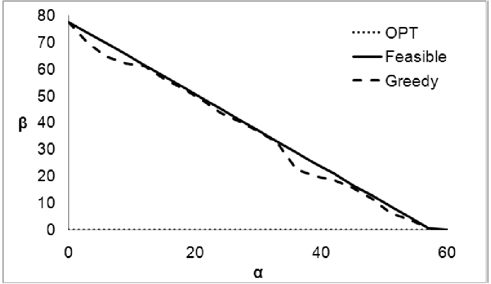
The simulation results are shown in Fig. 6. For both cases of exponential and logarithmic functions, the achievable regions of the OPT policy are rectangles. That is because the OPT policy only aims at maximizing the total per-period rewards and does not allow any tradeoff between rewards of different tasks. The achievable regions of the OPT policy are also much smaller than the feasible regions. On the other hand, the achievable regions of the Greedy Maximizer are very close to the feasible region for both the cases of exponential and logarithmic functions. Also, its achievable regions are strictly larger than that of the OPT policy. This also shows that the Greedy Maximizer can provide fine-grained tradeoff between tasks.

The most surprising result is that for linear functions. In this case, the OPT policy fails to fulfill any pairs of $(\alpha,\beta)$ except $(0,0)$ . A closer examination on the simulation result shows that, besides mandatory parts, the OPT policy only schedules optional parts of tasks $D$ and $F$ . This example shows that, in addition to restricted achievable regions, the OPT policy can also be extremely unfair. Thus, the OPT policy is not desirable when fairness is concerned. On the other hand, the achievable region of the Greedy Maximizer is almost the same as the feasible region. These simulation results also suggest that although we have only proved that the Greedy Maximizer is a 2-approximation policy, this approximation bound is indeed very pessimistic. In most cases, the performance of the Greedy Maximizer is not too far from that of a feasibility optimal policy.

Next, we simulate a system in which all tasks have the same period. We assume that $\tau_{X}=120$ , $m_{X}=0$ , and $o_{X}=120$ for all $X\in S$ . We also simulate all the three functions, exponential, logarithmic, and linear. Detailed parameters are shown in Table II.

Task id	$f^{1}_{X}(t)$	$f^{2}_{X}(t)$	$f^{3}_{X}(t)$	$\hat{q}^{*}_{X}$
A	$15(1-e^{-t/15})$	$7\ln(3t+1)$	$5t$	$5\alpha$
B	$20(1-e^{-3t/8})$	$10\ln(10t+1)$	$7t$	$7\alpha$
C	$4(1-e^{-t/5})$	$2\ln(3t+1)$	$t$	$\alpha$
D	$10(1-e^{-t/30})$	$5\ln(15t+1)$	$4t$	$4\beta$
E	$5(1-e^{-t/5})$	$3\ln(20t+1)$	$2t$	$2\beta$
F	$8(1-e^{-t/20})$	$4\ln(6t+1)$	$3t$	$3\beta$

TABLE II: Task parameters for a system in which all tasks have the same period.

The simulation results are shown in Fig. 7. As in the previous simulations, the achievable regions of the Greedy Maximizer are always larger than those of the OPT policy, for all functions. Further, the achievable regions of the Greedy Maximizer are exactly the same as the feasible regions. This demonstrates that the Greedy Maximizer fulfills every strictly feasible system when the periods of all tasks are the same.

VIII Concluding Remarks

We have studied a model in which a system consists of several periodic real-time tasks that have their individual reward requirements. This model is compatible with both the imprecise computation models and IRIS models. By making each task specify its own reward requirement, our model can offer better fairness, and it allows tradeoff between tasks. Under this model, we have proved a necessary and sufficient condition for feasibility, and designed a linear time algorithm for verifying feasibility. We have also studied the problem of designing on-line scheduling policies and obtained a sufficient condition for a policy to be feasibility optimal, or to achieve an approximation bound. We have then proposed a simple on-line scheduling policy. We have analyzed the performance of the on-line scheduling policy and proved that it fulfills all feasible systems in which the periods of all tasks are the same. For general systems where periods may be different for different tasks, we have proved that the on-line policy is a 2-approximation policy. We have also conducted simulations and compared our on-line policy against a policy that maximizes the total reward in the system. Simulation results show that the on-line policy has much larger achievable regions than that of the compared policy.

Acknowledgement

The authors are grateful to Prof. Marco Caccamo for introducing us to this line of work.

References

[1] H. Aydin, R. Melhem, D. Mosse, and P. Mejia-Alvarez, “Optimal reward-based scheduling for periodic real-time tasks,” IEEE Transactions on Computers, vol. 50, pp. 111–130, February 2001.
[2] J.-T. Chung, J. W. S. Liu, and K.-J. Lin, “Scheduling periodic jobs that allow imprecise results,” IEEE Transactions on Computers, vol. 39, pp. 1156–1174, September 1990.
[3] J. W. Liu, K.-J. Lin, W.-K. Shih, and A. C.-S. Yu, “Algorithms for scheduling imprecise computations,” Computers, vol. 24, pp. 58–68, May 1991.
[4] W.-K. Shih and J. W. Liu, “Algorithms for scheduling imprecise computations with timing constraints to minimize maximum error,” IEEE Transactions on Computers, vol. 44, pp. 466–471, March 1995.
[5] P. H. Feiler and J. J. Walker, “Adaptive feedback scheduling of incremental and design-to-time tasks,” in Proceedings of the 23rd International Conference on Software Engineering, pp. 318–326, 2001.
[6] P. Mejia-Alvarez, R. Melhem, and D. Mosse, “An incremental approach to scheduling during overloads in real-time systems,” in Proceedings of the 21st IEEE Real-Time Systems Symposium, pp. 283–293, 2000.
[7] J.-M. Chen, W.-C. Lu, W.-K. Shih, and M.-C. Tang, “Imprecise computations with deferred optional tasks,” Journal of Information Science and Enginnering, vol. 25, no. 1, pp. 185–200, 2009.
[8] M. Zu and A. M. K. Chang, “Real-time scheduling of hierarchical reward-based tasks,” in Proceedings of the 9th IEEE Real-Time and Embedded Technology and Applications Symposium, pp. 2–9, 2003.
[9] M. Amirijoo, J. Hansson, and S. H. Son, “Specification and management of QoS in real-time databases supporting imprecise computations,” IEEE Transactions on Computers, vol. 55, pp. 304–319, March 2006.
[10] J. K. Dey, J. Kurose, and D. Towsley, “On-line scheduling policies for a class of IRIS (increasing reward with increasing service) real-time tasks,” IEEE Transactions on Computers, vol. 45, pp. 802–813, July 1996.
[11] H. Cam, “An on-line scheudling policy for IRIS real-time composite tasks,” The Journal of Systems and Software, vol. 52, pp. 25–32, 2000.
[12] B. Korte and J. Vygen, Combinatorial Optimization, Theory and Algorithms. Springer-Verlag Berlin Heifelberg, 2008.