Quickest Detection with Social Learning: Interaction of local and global decision makers
Abstract
We consider how local and global decision policies interact in stopping time problems such as quickest time change detection. Individual agents make myopic local decisions via social learning, that is, each agent records a private observation of a noisy underlying state process, selfishly optimizes its local utility and then broadcasts its local decision. Given these local decisions, how can a global decision maker achieve quickest time change detection when the underlying state changes according to a phase-type distribution? The paper presents four results. First, using Blackwell dominance of measures, it is shown that the optimal cost incurred in social learning based quickest detection is always larger than that of classical quickest detection. Second, it is shown that in general the optimal decision policy for social learning based quickest detection is characterized by multiple thresholds within the space of Bayesian distributions. Third, using lattice programming and stochastic dominance, sufficient conditions are given for the optimal decision policy to consist of a single linear hyperplane, or, more generally, a threshold curve. Estimation of the optimal linear approximation to this threshold curve is formulated as a simulation-based stochastic optimization problem. Finally, the paper shows that in multi-agent sensor management with quickest detection, where each agent views the world according to its prior, the optimal policy has a similar structure to social learning.
Index Terms:
Quickest time Bayesian change detection, social learning, phase-type distribution, stochastic dominance, Blackwell dominance, multi-agent sensor scheduling, partially observed Markov decision processI Introduction
Classical Bayesian quickest time detection [43, 44] involves detecting a geometrically distributed change time by optimizing the tradeoff between false alarm frequency and delay penalty. The literature is vast, with applications in biomedical signal processing, machinery monitoring and finance [39, 8, 34, 44], see also [37] for team detection, and [52, 53]. Classical quickest detection can be formulated as the following sequential protocol involving a countable number of agents: Suppose each agent acts once in a pre-determined sequential order indexed by . Agent receives an observation of the underlying state at time and computes the posterior probability that the state has changed. It then reveals this posterior probability to subsequent agents. This process repeats until a stopping time at which the global decision maker announces a change. It is well known [43, 44] that the optimal policy to declare a change has a threshold (monotone) structure: if the posterior probability (belief state) exceeds a threshold, then a change is announced; otherwise agents continue making observations.
I-A Context
Motivated by understanding how local decisions affect global decision-making in multi-agent systems, this paper considers a generalization of the above classical quickest detection setup. Given local decisions from agents that are performing social learning, how can a global decision maker achieve quickest time change detection? In other words, how can a stochastic control problem (stopping time problem) be solved to make global decisions based on local decisions of agents? We consider phase-type distributed change times and interaction between local and global decision-makers as outlined in the following two examples:
Example 1. Social Learning based Quickest-time detection: Suppose that a multi-agent system performs social learning [12]11 1 Another way of viewing the social learning model is that there are finite number of agents that act repeatedly in some pre-defined order. If each agent picks its local decision using the current public belief, then the setup is identical to the social learning setup. We also refer reader to [1, 2] for several recent results in social learning over several types of network adjacency matrices. to estimate an underlying state as follows: Just as in the classical quickest detection protocol above, agents act sequentially in a pre-determined order. However, instead of revealing its posterior distribution of change, each agent reveals its local decision to subsequent agents. The agent chooses its local decision by optimizing a local utility function (which depends on the public belief of the state and its local observation). Subsequent agents update their public belief based on these local decisions (in a Bayesian setting), and the sequential procedure continues. Given these local decisions, how can such a multi-agent system detect a change in the underlying state and make a global decision to stop?
Example 2: Quickest-time detection with adaptive sensing: Consider a multi-sensor system where each adaptive sensor is equipped with a local sensor manager (controller). The multi-sensor system acts sequentially as follows: Based on the existing belief of the underlying state, the local sensor-manager chooses (adapts) the sensor mode e.g., low resolution or high resolution. The sensor then views the world based on this mode. Given the belief states and local sensor-manager decisions, how can such a multi-agent system achieve quickest time change detection?22 2 The information flow patterns of Example 1 and 2 are similar. In Example 1, the sequence of events is . In Example 2, the sequence of events is . Quickest detection with such sensor management is of importance in automated tracking and surveillance systems [3, 5, 14]. In such cases, if individual agents or cluster heads are polled sequentially (e.g. round-robin fashion) then the resulting dynamics are very similar to the social learning setup.
Classical quickest detection is a trivial case of the above examples where agents reveal their local observation (instead of local decision) to subsequent agents. The above examples are non-trivial generalizations due to the interaction of the local and global decision makers33 3 A signal processing interpretation of social learning is as follows. Instead of using the posterior distribution to achieve quickest time detection, the decision maker (or individual agents) computes the maximum aposteriori (MAP) estimate of the underlying state at each time instant. Given these hard decision MAP state estimates (local decisions), how can the global decision maker achieve quickest change detection?. In both examples, the local decision determines the belief state which determines the global decision (stop or continue) which determines the local decision at the next time instant and so on. This interaction of local and global decision-making leads to discontinuous dynamics for the posterior probabilities (belief state) and unusual behavior as outlined below. We will show that the optimal decision policy has multiple thresholds and the stopping regions are non-convex.
Fig.1(a) gives a visual description of the optimal policy of social learning based quickest detection. It illustrates a triple threshold policy for geometric distributed change time. Complete details of this numerical example are given in Sec.VII. The horizontal axis is the posterior probability of no change. The vertical axis denotes the optimal decision: denotes stop and declare change, while denotes continue. The multi-threshold behavior of Fig.1(a) is unusual: if it is optimal to declare a change for a particular posterior probability, it may not be optimal to declare a change when the posterior probability of a change is larger! Thus, the global decision (stop or continue) is a non-monotone function of the posterior probability obtained from local decisions. Fig.1(b) shows the associated value function obtained via stochastic dynamic programming. Unlike standard sequential detection problems where the value function is concave, the figure shows that the value function is non-concave and discontinuous. To summarize, Fig.1 shows that social learning based quickest detection results in fundamentally different decision policies compared to classical quickest time detection (which has a single threshold). Thus making global decisions (stop or continue) based on local decisions (from social learning) is non-trivial.


I-B Motivation and Related Works
Social Learning: In the last decade, social learning has been studied widely in economics to model the behavior of financial markets, crowds and social networks, see [1, 2, 12, 46, 31] and numerous references therein. The social learning framework is similar to Hellman’s and Cover’s seminal papers [15, 19] which analyze learning with limited memory. [12, Chapters 3 and 4] gives an excellent exposition of social learning. An important result in social learning [6, 10] is that if the underlying state is a random variable and the observation and local decision spaces are finite, then agents eventually herd and end up making the same local decision irrespective of their observation. Such information cascades have been used in [12] to model sequences of financial trades, crashes and booms, and auctions. There is strong motivation to understand the interaction of local and global decision makers in social learning. Global decision making with social learning has recently been studied by several economists; for example [13, 11, 12, 45, 26] describe how information externalities affect global and local decision making in social learning. The current paper can be viewed as addressing a related problem: if individual agents make (simple) decisions by optimizing a local utility, how can the global system achieve the (complex) task of detecting a change. In a non-Bayesian setting such problems of designing sophisticated global behavior given simple local behavior have also been studied in game-theoretic learning [18, 17, 27] involving correlated equilibria.
PH-distributed change time: This paper deals with quickest detection for PH-distributed change times. PH-distributions are used widely in queuing theory [36] and include geometric distributions as a special case. The optimal detection of a PH-distributed change point is useful since the family of all PH-distributions forms a dense subset for the set of all distributions, i.e., for any given distribution function such that , one can find a sequence of PH-distributions to uniformly approximate over ; see [36]. Therefore there is strong motivation to analyze quickest detection with PH-distributed change times and social learning. Quickest time change detection for PH-distributed change times is analyzed in [26]. The current paper generalizes these results to include social learning. A systematic investigation of the statistical properties of PH-distributions can be found in [36].
I-C Main Results and Organization
This paper deals with characterizing the structure of the global quickest-time change detection policy in multi-agent
systems where individual agents make local myopic decisions when performing social learning.
The main results and organization of the paper are as follows:
1. Multi-agent Protocol: Sec.II presents the multi-agent social learning protocol. The quickest time detection
problem is formulated. We also point out in (21) the difference between the social learning model
and the classical Kolmogorov-Shiryaev model for quickest change detection.
2. Dynamic Programming Formulation and Dominance of Classical Detection:
In Sec.III, the optimal stopping policy is characterized in terms of stochastic dynamic programming.
It is shown that the value function is in general non-concave. Also Theorem 1 uses Blackwell ordering of measures to show that the optimal cost incurred in social learning based quickest detection
is always
larger than classical quickest detection. Although such a result might appear intuitive (decision making using social learning is based on less information than classical quickest detection), the proof
is nontrivial. One needs to show that the expected cost of the entire trajectory of a stochastic
dynamical system (driven by the social learning protocol) is larger than that of classical quickest detection.
3. Main assumptions and Multi-threshold Policies: Sec.IV starts
with the main assumptions required to analyze the structure of the optimal quickest detection policy.
These assumptions allow us to decompose the belief
space into polytopes (Theorem 2). On each of these polytopes, the conditional probability of a local decision given the underlying
state and posterior distribution is a constant.
The main result of Sec.IV is to
characterize quickest time change detection
policies when the probability of change, denoted , is small. When the probability of change equal to zero, Theorem 3 characterizes explicitly
the multi-threshold structure of the optimal decision policy and
non-concave behavior of the value function for sequential detection of a fixed state.
Then
Corollary 1 shows that the optimal quickest-time detection policy for change probability ,
yields a cost that is within
of the optimal cost for zero change probability.
An important ingredient in the proof of this
result is characterization of fixed points of the social learning filter update (Lemma 2) which
also characterizes regions where the agents form information cascades in social learning.
4.
Phase-type Distributed Change Times:
The next main result is to
is to characterize the optimal policy of the global decision maker to achieve quickest time detection when the change time has a phase-type (PH) distribution and
individual agents are performing social learning.
As mentioned above, PH-distributions can approximate arbitrary distributions and so are widely used in discrete-event systems.
A PH-distributed change time can be modelled as a multi-state Markov chain with an absorbing state, see [26] and also [36] for a systematic description. (For a 2-state Markov chain, the PH-distribution specializes to the geometric distribution). So for quickest time detection with PH-distributed change time, the belief states (Bayesian posterior) lie in a multidimensional simplex of probability mass functions.
Under what conditions will there exist a threshold stopping policy for quickest detection with PH-distributed change time and social learning? Under what conditions for the geometric change time case does the optimal policy coincide with the classical Kolmogorov-Shiryaev model?
To answer these questions, the main results of Sec.V are as follows:
(i) Theorem 4 gives sufficient conditions under which the optimal decision policy
for the global decision maker is myopic and characterized by a linear threshold hyperplane
in the multidimensional simplex. For the geometric case, this results yields an identical threshold to the Kolmogorov-Shiryaev model.
(ii) Theorem 5 gives sufficient conditions so that the optimal decision policy is characterized by a single switching curve
in the multidimensional simplex. The result uses lattice programming [49] and structural results involving
monotone likelihood ratio stochastic orders [40, 28], and a novel modification of it.
The result is useful because it implies that the global decision to stop
can be implemented efficiently at each agent. Each agent simply needs to compare its belief state with respect to the
threshold curve (in terms of a monotone likelihood ratio partial order on the space of posterior distributions).
Theorem 7 gives sufficient
conditions on the optimal linear approximation to this curve that preserves the monotone likelihood ratio increasing
structure of the optimal decision policy. This linear approximation can be estimated
via simulation based stochastic optimization.
5. Multi-agent Quickest Time Detection with active sensing: Sec.VI considers multi-agent quickest time detection outlined in Example 2 above.
We show that the optimal policy is similar to that in social learning based quickest detection.
II Social Learning Model and Protocol for Quickest Time Detection
In this section, the multi-agent social learning model is presented in Sec.II-A. This constitutes the local decision-making framework for estimating an underlying state. Then Sec.II-B formulates the costs incurred by the global decision maker in quickest time detection. Sec.II-C presents the global quickest time detection objective. Finally, Sec.II-D summarizes the entire social learning quickest detection model.
II-A The Multi-agent Social Learning Model
Consider a countably infinite number of agents44 4 As mentioned earlier, the same setup holds if a finite number of agents are polled repeatedly in some pre-defined order, providing each agent picks its local decision based on the most recent public belief. performing social learning to estimate an underlying state process . Each agent acts once in a predetermined sequential order indexed by . The index can also be viewed as the discrete time instant when agent acts.
Let denote the local (private) observation of agent and denote the local decision agent takes. Define the sigma algebras:
| (1) |
1. Absorbing-state Markov chain and Phase-Type Distribution Change Times: The state represents the underlying process that changes at time . We model the change point by a phase type (PH) distribution. As mentioned in Sec.I PH-distributions form a dense subset for the set of all distributions [36] and so can be used to approximate change times with arbitrary distribution. This is done by constructing a multi-state Markov chain as follows: Assume the underlying state evolves as a Markov chain on the finite state space . Here state ‘1’ is an absorbing state and denotes the state after the jump change. The states can be viewed as a single composite state that resides in before the jump.
The initial distribution is , . We are only interested in the case where the change occurs after a least one measurement, so assume . So the transition probability matrix is of the form
| (2) |
Let the “change time” denote the time at which enters the absorbing state 1, i.e.,
| (3) |
The distribution of the change time is equivalent to the distribution of the absorption time to state 1 and is given by
| (4) |
where . So by appropriately choosing the pair and state space dimension , one can approximate any given discrete distribution on by the distribution ; see [36, 240-243]. To ensure that is finite, we assume states are transient. In the special case when is a 2-state Markov chain, the change time is geometrically distributed.
2. Local Observation: Agent’s local (private) observation is obtained from the observation likelihood distribution
| (5) |
The states are fictitious and are defined to generate the PH-distributed change time . So states are indistinguishable in terms of the observation . That is, for all .
3. Private belief: Using local observation , agent updates its private belief defined as
| (6) |
Thus the private belief is the posterior distribution of the underlying state given the past local decisions and current observation. It is computed by agent according to the following Hidden Markov Model (HMM) filter:
| (7) | ||||
Also denotes the public belief available at time (defined in Step 5 below).
4. Agent’s local decision: Agent then makes local decision to minimize myopically its expected cost. To formulate this, let denote the non-negative cost incurred if the agent picks local decision when the underlying state is . Denote the local decision -dimensional cost vector
| (8) |
Then agent chooses local decision greedily to minimize its expected cost:
| (9) |
In quickest change detection, since states are indistinguishable in terms of observation , we assume that for each .
5. Social learning Public Belief: Finally agent broadcasts its local decision . Subsequent agents use decision to update their public belief of the underlying state as follows: Define the public belief as the posterior distribution of the state given all local decisions taken up to time .
| (10) |
Then agents update their public belief according to the following “social learning Bayesian filter”:
| (11) |
We use the notation to point out that the above Bayesian update map depends explicitly on the belief state . (For notational simplicity we have chosen not to use the superscript for ). This is a key difference compared to the HMM filter (7) where the Bayesian update map does not depend explicitly on belief state . In (11), denotes the diagonal matrix where
| (12) |
denotes the conditional probability that agent chose local decision given state . We call as the local decision likelihood probabilities in analogy to observation likelihood probabilities (5) in classical filtering.
Clearly observing the local decision taken by agent yields information about its local observation . That is, serves as a surrogate observation of the underlying state . The following lemma summarizes how subsequent agents use to compute the local decision likelihood probabilities in the social learning filter. The proof is straightforward and omitted.
Lemma 1.
The main implication of Lemma 1 is that the social learning Bayesian filter (11) is discontinuous in the belief state , due to the presence of indicator functions in (13). The likelihood probabilities in (12) are an explicit function of the belief state – this is stark contrast to the standard quickest detection problems where the observation distribution is not an explicit function of the posterior distribution.
Summary: A key aspect of the information pattern in the above social learning protocol is that agent does not have access to the private belief state or private observations of previous agents. Instead each agent only has access to the local decisions taken by previous agents together with its own current private observation . The fact that the likelihood probabilities is an explicit function of the public belief state (see (13)) is an important aspect of social learning that is not present in classical sequential detection problems. It makes the Bayesian update of the public belief discontinuous with and makes our proofs substantially harder than standard concavity arguments in classical quickest detection problems.
Belief State Space: Before proceeding with the quickest time detection formulation, we briefly describe the space in which the public belief defined in (10) lives. The public belief belongs to the unit dimensional simplex denoted as
| (14) |
So for geometric-distributed change times, the belief state space is the interval . For PH-distributed change times, the belief space is a multi-dimensional simplex. For example, is a two-dimensional unit simplex (equilateral triangle); is a tetrahedron, etc. The vertices of the unit simplex are the unit -dimensional vectors , where
| denotes the unit vector with in the th position, . | (15) |
Of course the private belief (6) also lives in .
II-B Quickest Time Detection: Costs Incurred by Global Decision Maker
With the above social learning based local decision framework, we now formulate the quickest time detection problem faced by the global decision maker. At each time , given the public belief , let denote the global decision taken:
| (16) |
Thus the global decision is measurable, where is defined in (1). In (16), the policy belongs to the class of stationary decision policies denoted . Below we formulate the costs incurred when taking these global decisions .
(i) Cost of announcing change and stopping: If global decision is chosen, then the social learning protocol of Sec.II-A terminates. If is chosen before the change point , then a false alarm penalty is incurred. The false alarm event represents the event that a change is announced before the change happens at time . To evaluate the false alarm penalty, let denote the cost of a false alarm in state , , where . Of course, since a false alarm is only incurred if the stop action is picked in states . The expected false alarm penalty is
| (17) |
The false alarm vector is chosen with increasing elements so that states further from state 1 incur larger penalties. (Obviously since ).
(ii) Delay cost of continuing: If global decision is taken then the social learning protocol of Sec.II-A continues to time . A delay cost is incurred when the event occurs, i.e., no change is declared at time , even though the state has changed at time . The expected delay cost is
| (18) |
where denotes the delay cost and is defined in (15).
Remarks: (i) Recall that the public belief state depends on the local decisions . Also the choice of global decision
determines when the local decision process terminates. This links
the local and global decision makers.
(ii) The above costs (17), (18) should be viewed as an example only.
The results of this paper also apply to more general stopping time problems with minor modifications if the global decisions are measurable (instead of
measurable), where and are defined in (1).
More generally, can also include the local decision cost incurred in social learning, see
remark at the end of Sec.V-B.
II-C Quickest Time Detection Objective
Let be the underlying measurable space where is the product space, which is endowed with the product topology and is the corresponding product sigma-algebra. For any , and policy , there exists a (unique) probability measure on , see [20] for details. Let denote the expectation with respect to the measure .
Let denote a stopping time adapted to the sequence of -algebras , see (1). That is, with determined by decision policy (16),
| (19) |
For each initial distribution , and policy , the following cost is associated:
| (20) |
Here denotes an economic discount factor. Since , are non-negative and bounded for all , stopping is guaranteed in finite time, i.e., is finite with probability 1 for any (including ).
Kolmogorov–Shiryaev criterion: Suppose implying that the change time is geometrically distributed. Choose the false alarm vector where is a positive constant, delay cost (18), and discount factor . Then the quickest time objective (20) assumes the classical Kolmogorov–Shiryaev criterion for detection of disorder [43]:
| (21) |
However, unlike classical quickest detection, the posterior (public belief) has discontinuous dynamics given by the social learning Bayesian filter (11). (Recall from (11), (13) that the dynamics of public belief depend on the local decision costs ).
II-D Summary
In summary, the social learning based quickest detection problem with PH-distributed change time is specified by the model
| (22) |
where is the transition probability matrix (2), is the private observation matrix (5), are the local decision costs (8), defined in (24) is the transformed global decision cost vector for quickest detection (in terms of false alarm (17) and delay penalty (18)), and is the discount factor (20). Also is the state space, is the private observation space, is the local decision space and is the global decision space.
III Stochastic Dynamic Programming Formulation and Dominance of Classical Quickest Detection
Sec.III-A formulates the optimal decision policy for social learning based quickest detection as the solution of a stochastic dynamic programming problem. Sec.III-B describes why social learning based quickest detection is a non-trivial extension of the standard quickest detection problem. Finally, Sec.III-C presents our first structural result – it uses Blackwell dominance of measures to show that optimal cost incurred in quickest time detection with social learning is always larger than that with classical quickest detection.
III-A Stochastic Dynamic Programming Formulation
Given the stopping time problem (20), it is well known [33] that the optimal policy can be expressed as the solution of a stochastic dynamic programming problem in terms of the belief state . Our characterization of the structure of the optimal policy will be based on analyzing the structure of this dynamic programming problem.
The optimal stationary policy and associated value function of the stopping time problem (20) are the solution of “Bellman’s dynamic programming equation”
| (23) | ||||
Here the global decision maker’s costs are defined in (17), (18), is the public belief Bayesian update (11), and the measure is defined in (11).
For our subsequent analysis, it is convenient to rewrite Bellman’s equation as follows. Define the transformed value function and global decision costs , and as follows:
| (24) | ||||
Then clearly satisfies Bellman’s dynamic programming equation
| (25) | ||||
| where |
The above transformation55 5 This transformation is used in [21, pp.389] to deal with stopping time problems. As a result of this transformation, the initial condition of the value iteration algorithm is modified, see (27). is convenient since the transformed stopping cost and in (24) captures all the costs involved in quickest detection. Of course, the optimal policy and hence stopping set remain unchanged with this coordinate transformation. The goal for the global decision-maker is to determine the optimal stopping set denoted . That is, is the set of public belief states for which it is optimal to declare a change and stop:
| (26) |
Value Iteration Algorithm
Let denote iteration number (the fact that we used previously to denote time should not result in confusion). The value iteration algorithm is a fixed point iteration of Bellman’s equation (25) and proceeds as follows: and
| (27) |
Let denote the set of bounded real-valued functions on . Since , , , are bounded, the value iteration algorithm (27) will generate a sequence of lower semi-continuous value functions that will converge pointwise as to , the solution of Bellman’s equation, see [9, Prop.1.3, Chap 3, Vol.2]
Since the belief state space in (14) is a unit simplex, the value iteration algorithm (27) does not yield a practical solution methodology for computing stopping set since needs to be evaluated on the continuum . Although Bellman’s equation and the value iteration algorithm is not useful from a computational point of view, in subsequent sections, we exploit its structure to characterize the stopping set in (26). We then exploit this structure to devise stochastic gradient algorithms for approximating the optimal policy and thus determining the stopping set .
III-B Why Social Learning based Quickest Detection is non-trivial
Let us illustrate why social learning based quickest detection results in a non-trivial behavior. We will show in Sec.IV that the belief space can be decomposed into polytopes denoted such that on each of these polytopes , the belief state update . Consider the value iteration algorithm (27) which is used as a basis for mathematical induction to prove properties associated with Bellman’s equation (25). It can be expressed as66 6 Note that from (27), is positively homogeneous, that is, for any , . So choosing which is the denominator term of in (11) yields the expression in the second equality of (28).
| (28) |
It should be clear from (28) that if is assumed to be concave on , is not necessarily concave on . In fact, even if is assumed to be concave in just one of the polytopes, say polytope , then is not necessarily concave on , since in (28) may map two distinct belief states in polytope to two different polytopes. As will be shown in numerical examples, in general will be discontinuous and non–concave.
Classical quickest detection problems are special instances of partially observed Markov decision process (POMDP) stopping time problems [26]. In POMDPs, the belief state update is not an explicit function of belief state since the observation probabilities are not an explicit function of . For such POMDP stopping time problems the value iteration algorithm reads77 7 We use the notation to denote the value function of the classical stopping problem. This will be defined formally in Sec.III-C where we will show , i.e., quickest detection with social learning always incurs a higher optimal cost than classical quickest detection.
and is to be compared with (28). Since the composition of a concave function with a linear function preserves concavity, it is easily seen that if is piecewise linear and concave, then so is . So by mathematical induction on the value iteration algorithm, and since the sequence converges pointwise (actually uniformly for POMDPs) to , the value function is concave and the stopping set is a convex (and therefore connected) set [32]. The key difference in the above social learning quickest detection formulation is that the local decision likelihoods (13) and therefore social learning filter are explicit and discontinuous functions of . This results in a possibly non-concave value function making determining non-trivial.
III-C Quickest Time Detection with Social Learning is More Expensive
This section presents our first main result. We prove that quickest detection with social learning is always more expensive than classical quickest detection. In social learning, agents have access to local decisions of previous agents instead of the actual observations. Thus one would expect intuitively that this information loss results in less efficient quickest time change detection compared to classical quickest detection. Here we confirm this intuition. The main idea is to use Blackwell dominance of observation measures.
III-C1 Notation
First define the optimal policy and cost in classical quickest time detection. Similar to (25), the optimal policy and cost incurred in classical quickest detection, satisfies the following Bellman’s equation:
| (29) | ||||
Recall is the Hidden Markov Model Bayesian filter defined in (7). Thus the only difference between the classical and social learning quickest detection problems is the update of the belief state, namely (7) in the classical setup versus (11) in the social learning formulation.
III-C2 Main Result
The following theorem says that if the initial belief state is chosen from any of the polytopes , the optimal detection policy with social learning incurs a higher cost than classical quickest detection.
Theorem 1.
Consider the social learning quickest time detection problem in (22) and associated value function in (25). Consider also the classical quickest detection problem with value function in (29). Then for any initial belief state , the optimal cost incurred by classical quickest detection is smaller than that of quickest detection with social learning. That is, .
Since the theorem holds for the case (equal number of local decision choices and observation symbols), a naive explanation that information is lost due to using fewer symbols in compared to is not true.
The proof of Theorem 1 is given in Appendix A-B. Recall from (13) that where and are stochastic matrices. Thus observation with conditional distribution specified by is said to be more informative than (Blackwell dominates) observation with conditional distribution , see [40]. The main idea in the proof is that under the assumptions of Theorem 1, the value function is concave for . Then the result is established using Jensen’s inequality together with Blackwell dominance on the Bellman’s equation. value iteration algorithm proves the result.
The first instance of a similar proof using Blackwell dominance for POMDPs was given in [50], see also [40], where it was used to show optimality of certain myopic policies. Our use of Blackwell dominance in Theorem 1 is somewhat different since we are using it to compare the value functions of two different dynamic programming problems. A useful consequence of Theorem 1 is that performance analysis of standard quickest detection problems [48] readily applies to form a lower bound for the cost incurred in social learning based quickest detection.
IV Assumptions and Quickest Detection with Small Change Probabilities
This section comprises of two parts.
(i) Sec.IV-A lists the main assumptions (A1), (A2), (S) which result in a natural partition of
belief space into convex polytopes with decision likelihoods (defined in (13)) being a constant (with respect to on
each polytope (Theorem 2). These polytopes play an important role in specifying the global quickest detection policy in the rest of the paper.
(ii) Sec.IV-B considers quickest time change detection with geometric distributed change time and gives explicit
conditions for the optimal policy to have a double threshold. In particular, Theorem 3 and Corollary 1 show that the optimal quickest-time detection policy for change probability ,
yields a cost that is within of the optimal cost for sequential detection of a constant state.
IV-A Polytope Structure and Main Assumptions
Since the public belief state is continuum (see (14)), as a first step in characterizing the optimal policy , we need to understand the structure of the decision likelihood probabilities defined in (13). Even though the belief state is continuum, it turns out that there are only possible local decision likelihood probability matrices . Let , denote the elements of the power set of (excluding, of course, the empty set). Define the following convex polytopes , :
| (30) |
Recall the local cost vectors are defined in (8). Then from (13) it follows that and hence is a constant on each polytope . Specifically, for rows , and for rows , .
Although in general there are possible matrices, we now show that by introducing assumptions (A1), (A2) and (S) below, there are only distinct local decision likelihood matrices . This forms an important preliminary step for characterizing the optimal global decision policy.
Recalling the notation in Sec.II-A, we list the following assumptions.
- (A1)
- (A2)
The transition probability matrix is TP2. (All second order minors of are non-negative).
- (A3)
The elements of vector in (24) are decreasing. A sufficient condition is that for and the false alarm vector and delay penalty satisfy and .
- (S)
Discussion of Assumptions:
Assumption (A1): The requirement that is TP2 with respect to states and
holds for numerous examples,
see Karlin’s classic book [22] and also [23]. Examples include quantized Gaussians, quantized exponential distributions,
Binomial, Poisson, etc.
For example consider quantized Gaussians.
Suppose where
, ,
and . Then
(A1) holds.
Assumption (A2) always holds trivially for . For , see [16, 25] for numerous examples. Consider the tridiagonal transition probability matrix with for and . As shown in [16, pp.99–100], a necessary and sufficient condition for tridiagonal to be TP2 is that . Such a diagonally dominant tridiagonal matrix satisfies Assumption (A2).
Assumption (A3) is a sufficient condition for to be decreasing in with respect to the monotone likelihood ratio order. We will use (A3) in Sec.V to obtain sufficient conditions for a threshold policy. Assumption (A3) always holds for the geometric distributed change times (). For PH-distributed change times (), Assumption (A3) can be viewed as design constraints the decision maker needs to take into account so that quickest detection with PH-distributed change times has a threshold policy [26]. Feasible values for the elements of are straightforwardly obtained using a LP solver such as linprog in Matlab.
Assumption (S) is only required for the problem to be non-trivial. If (S) does not hold and for , then local decision will always dominate decision and the problem reduces to a standard quickest detection problem where the observed local decision yields no information about the state. Assumption (S) implies is decreasing in , i.e., the local cost is submodular which implies the zero crossing condition that is important in the proof of Theorem 2.
The following theorem is an abbreviated version of Theorem 2 presented in Appendix A-C. It will be used in the rest of the paper as a natural partition of the belief state space . Recall that transition probability , observation probability matrix and local cost vector are defined in (2), (7), (8) respectively.
Theorem 2.
As a consequence of Theorem 2 and (13), there are only possible decision likelihood matrices , one per polytope , . We will denote these decision likelihood matrices as
| (32) |
Example: To give some insight into the structure of decision likelihood matrix , suppose (state space), (observation space), (local decision space). Then assuming (A1), (A2), (S), by Theorem 2 there are up to convex polytopes. The matrices defined in (13), (32) are
| (33) |
Then from (32) the 4 possible decision likelihood matrices are
| (34) |
The detailed version of Theorem 2 in Appendix A-C guarantees that each of these matrices is TP2. Fig.2 illustrates these polytopes and hyperplanes defined below.


Let us give some intuition behind Theorem 2. Define the following hyperplanes that are subsets of :
| (35) |
The main intuition of the above theorem is that (A1), (A2), (S) imply that satisfies a single crossing condition [4] with respect to , see Definition 5 in Appendix A-A. This means that the set of belief states satisfy the following subset property:
| (36) |
This implies that the hyperplanes , , do not intersect within the simplex . It is nice that straightforward conditions such as (A1), (A2), (S) ensure this. Otherwise dealing with intersecting hyperplanes in a multi-dimensional simplex can be a real headache. Theorem 2(iv) in Appendix A-C shows that each hyperplane partitions such that vertices lie on one side and lie on the other side. In Sec.V, we will introduce Assumption (PH)(ii) which ensures that always lie in polytope as illustrated in Fig.2.
IV-B Multi-Threshold Structure of Social Learning based Quickest Detection
The main result (Theorem 3 and Corollary 1) below gives sufficient conditions under which social learning based quickest detection has a double threshold policy. Consider the model in (22) with geometric change time:
| (37) |
with false-alarm vector in (17) and delay cost (18). Here the change probability is a small non-negative scalar. So the change time is geometrically distributed with .
The analysis in this subsection proceeds as follows:
Step 1: For , the problem becomes a simple sequential detection problem for state – we
explicitly
characterize the multi-threshold behavior of the optimal decision policy in Theorem 3 below.
Step 2:
It is then shown that for small , the optimal value function is within of the value function
for the case of zero change probability (Corollary 1). So, the optimal policy computed for zero change probability yields
performance that is close to that of the optimal quickest detection policy for small .
IV-B1 Step 1: Sequential Detection of State 1
In line with above plan, consider the sequential detection problem for state 1 with social learning formulated in Sec.II with
| (38) |
The state is a random variable chosen at with distribution and remains constant for . The goal is to detect and announce state if based on noisy observations. The global decision is a function of the public belief . The optimal policy that optimizes (20) satisfies Bellman’s equation (25).
The 2-dimensional belief state is parametrized by the scalar , i.e., is the interval . Each hyperplane (35) now is a point on the interval ; let the 2-dimensional vector denote the belief state corresponding to . The polytopes , , in Theorem 2 are now intervals which are subsets of . If (A1) and (S) hold, then , , .
To handle the discontinuity in the social learning filter (11), we start with the following lemma that characterizes useful structural properties of the social learning filter. First define the belief state
| (39) |
Lemma 2.
Consider the social learning filter (11) and assume
(A1), (S) hold. Then:
(i) .
(ii) If is symmetric, then and are fixed points of the composite Bayesian map:
| (40) |
The implication of the above lemma is that can be partitioned into 4 intervals, namely , , and . Fig.3 illustrates these regions and the dynamics specified in Lemma 2. The main result below characterizes the structure of the optimal global decision policy on these 4 intervals. The theorem also characterizes information cascades [12] (more colloquially “herding”) which is a salient feature of social learning.

Theorem 3.
Consider the sequential detection problem with parameters (38). Suppose agents
make local decisions via social learning.
Assume (A1), (S) hold. (Note (A2) holds trivially since ). The optimal global decision policy has the following properties:
(i) For , the global decision policy has a threshold structure:
| (41) |
Also for , the value function (25)
is where is defined in (24).
(ii)
The intervals and are “information cascades” [12]. That is, if , then and social learning ceases.
(iii) If is symmetric, then for , the global decision policy has the following structure:
(a) For , is concave and there is at most one interval where .
(b) For , is concave and there is at most one interval where .
The implication of Part (iii) of the above theorem is that the stopping set comprises of at most three intervals. One of these intervals is , with the threshold defined in (41). The second claim of the theorem follows, since if public belief , then the optimal local decision is irrespective of the observation . Similarly, if , then the optimal local decision is irrespective of the observation . Therefore when the public belief is in , the local decision of an agent reveals no information about its local observation to subsequent agents.
IV-B2 Step 2: Quickest Time Detection bound for small
Given the characterization in Theorem 3 of the optimal policy for , we now consider the quickest change detection problem for small specified in (37). It is convenient to introduce the following dependent notation.
Let denote the cost incurred by the optimal policy with transition matrix . We use the notation to denote the explicit dependence of the 3 intervals , , , defined in (31). For , we denote these intervals as . The following result bounds the difference between and . Note that is characterized in Theorem 3 and (identity matrix).
Recall from (23) that is the actual optimal expected cost associated with optimal decision policy . As mentioned below (25), the transformed value function is more convenient to deal with to prove the existence of optimal threshold policies and the optimal policy remains invariant to the transformation from to .
Corollary 1.
Consider the social learning based quickest detection model in (22) with probability of change specified in (37). Then, for initial belief , , the optimal policy (characterized in Theorem (3)) incurs a total global cost that constitutes an upper-bound to the optimal global cost incurred in the quickest detection problem. More specifically, for , ,
| (42) |
Discussion: The implication of (42) is that the simple policy of Theorem 3 is near optimal for quickest time detection with social learning when is small. Note that (42) compares the optimal costs in regions , , so we are omitting intervals where the models have different local decision likelihood probabilities . The regions we are omitting are in size. In each region , the only difference between the quickest detection model and the simplified model is the transition matrix ( vs ). This allows us to give a tight bound in the sense that for , the optimal costs and coincide. Of course, (42) requires the discount factor . We refer the reader to [48] for an alternative and more general approach.
The proof of Corollary 1 follows from Theorem 2 of [42]. In terms of our notation, Theorem 2 of [42] shows that for a POMDP with piecewise linear value function at each iteration of the value-iteration algorithm, for ,
| (43) |
where the induced matrix norm is with respect to the elements. Since from Theorem 3, the value function is piecewise linear, (43) applies. From the structure of in (37) and since , clearly


IV-B3 Numerical Example
Consider the social learning quickest detection model with ,
| (44) |
Fig.4 shows the optimal policies (Theorem 3) and (optimal quickest detection policy) together with optimal costs and for change probability . As can be seen the quickest detection optimal policy and costs are very close to the costs and policies specified by Theorem 3. For the policies and are almost identical and cannot be distinguished in Fig.4. The policies and optimal costs were obtained by running the value iteration algorithm for horizon 500 with discretized to a grid of 100 points.
V Quickest Time Detection for Geometric and PH-distributed Change Time
The previous section illustrated the multi-threshold behavior of social learning based quickest time change detection. What sufficient conditions on the social learning model lead to single threshold behavior? This section gives such conditions for PH-distributed change times modelled by a -state Markov chain. For geometric change times (i.e., these conditions yield a threshold that is identical to the classical Kolmogorov–Shiryaev criterion (21).
This section comprises of the following results.
(i) Sec.V-A gives sufficient conditions for
the optimal global decision policy to be myopic and characterized by a linear hyperplane threshold.
(ii) Sec.V-B gives less restrictive conditions under which the optimal policy is increasing
with respect to the monotone likelihood ratio (MLR) order and is characterized by a single threshold
curve.
Recall that for PH-distributed change time, the belief space is a multi-dimensional simplex.
To order posterior distributions on this simplex, the MLR stochastic order (which is a partial order)
will be used since it is preserved under conditional expectations.
The results involve analysis of the structure of the social learning Bayesian filter
together with lattice programming. All definitions of these orders and consequences are given in the
Appendix.
(iii) Sec.V-C describes how sufficient conditions can be given for multiple-threshold policies.
(iv) Finally, Sec.V-D characterizes the optimal
linear approximation to the MLR increasing policy. It then formulates estimation of the optimal linear approximation
to the threshold curve as a stochastic optimization problem.
Assumption (PH)
Recall fictitious states (corresponding to belief states ) are used to model the PH-distribution in (4). It therefore makes sense to constrain the model parameters so that the global decision policy at the belief states are identical (and similarly for the local decisions taken in social learning). Throughout this section, when considering PH-distributed change times, we make the following assumption.
- (PH)
(i) for . (ii) lie in polytope .
Assumption (PH)(i) says that the optimal policy
treats each of the fictitious states identically – they all
lie outside the stopping set . In similar vein, (PH)(ii) requires that individual agents making local decisions
treat the fictitious states identically, i.e., they lie to the left of each hyperplane , .
Obviously, (PH) holds trivially for (geometric case) - otherwise the quickest change problem would be degenerate.
V-A Case 1: Myopic Quickest Detection with Linear Hyperplane Threshold
The main result of this subsection is Theorem 4 which shows that under suitable conditions, the optimal policy has a myopic structure characterized by . Recall that in (24) denotes the transformed costs of the global decision maker with elements , . Denote the vertices of the intersection of the linear hyperplane with the facets of simplex as , . Then it is straightforwardly seen that these vertices are
| (45) |
Now introduce the following assumption:
- (C1)
for all , .
The relevance of (C1) is apparent from the following lemma (proof in Appendix A-E). Define the set of belief states (polytope)
| (46) |
Lemma 3.
Recall (A1), (A2), (A3) were introduced in Sec.IV-A and (PH) at the beginning of Sec.V. The main result is as follows. The proof is in Appendix A-E.
Theorem 4.
Consider the social learning based quickest time detection model in (22). Assume (A1), (A2), (A3), (S), (C1), (PH). Then the global decision maker’s optimal policy is myopic and is of the form
| (47) |
For the special case (geometric change time),
| (48) |
The above result is similar to the entry fee optimal stopping problem having a myopic policy discussed in [21, pp.389] and [41, Theorem 2.2, pp.54]. It is important to note, however, that even though the optimal policy in (47) is characterized by a linear threshold, the value function can still be discontinuous and non-concave (unlike classical stopping time problems). This will be illustrated in the numerical example below.
Let us illustrate what Theorem 4 says. Consider Fig.5. The shaded region in Fig.5 denotes the set . It is clear from Bellman’s equation (25) that the stopping set is a subset of this shaded region . What Theorem 4 says is that the stopping set is equal to the shaded region, i.e., , if (C1) and (PH) hold. In terms of Fig.5, (C1) is sufficient for to map the belief states and (which are the vertices of the line ) to polytope . (PH)(i) implies that states lie to the left of the line (which corresponds to the region ). Similarly, (PH)(ii) means that lie to the left of each line segment , , i.e., .
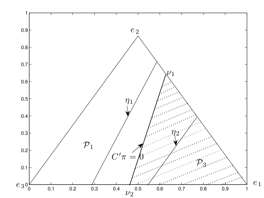
Numerical Example: To illustrate Theorem 4, consider the geometric change time model in (44) except that . Even though the sufficient condition (C1) does not hold, the optimal policy is characterized by a single threshold given by (48). This is shown in Fig.6. As can be seen in Fig.6, the value function is non-concave and discontinuous.


V-B Case 2: Existence of a single threshold switching curve
In this subsection, we consider another special case of the social learning based quickest detection model (22). Theorem 5 below shows that the stopping set is characterized by a single threshold curve on the belief space. The threshold coincides with the classical quickest time detection problem with non-informative observations. For PH-distributed change times, unlike the previous subsection, the threshold curve is not necessarily linear. We give a stochastic gradient algorithm to estimate this threshold curve in Sec.V-D.
V-B1 Structural Result
We make the following assumptions. Recall the global decision maker’s cost vector is defined in (24). Let , denote the vertices of the intersection of hyperplane (defined in (35)) with . These vertices are computed as (45) with replaced by .
- (C2)
for .
- (C3)
The linear hyperplane lies in polytope .
The following is the main result. The proof is in Appendix A-F.
Theorem 5.
Consider the social learning based quickest detection model in (22).
Assume (A1), (A2), (S) and (PH) hold. The optimal policy has the following structure
(i) Under (C3), for .
(ii) Under (C2) and (C3), the stopping set is as convex subset of polytope . Therefore the boundary of is differentiable almost everywhere.
(iii) For geometric-distributed change time (), under (C3), the optimal policy is identical to that of the Kolmogorov–Shiryaev criterion
(21) with uniformly distributed observation probabilities.
(iv) Under (A3), (C2), (C3).
on the polytope , has the following structure:
| (49) |
(The MLR order is defined in (61) in Appendix A-A). Hence the boundary of the stopping set within intersects any line segment or at most once (see geometric interpretation below).
V-B2 Discussion of Theorem 5 and assumptions
Assumption (C3) localizes the decision threshold to polytope . As a consequence of (C3), on all polytopes except . Therefore on these polytopes, . Thus statement (i) is obvious.
Assumption (C2) together with (A1), (A2), (S) and (PH) ensures that the polytope is closed under the belief state mapping . That is, implies for all . Note that Assumption (C2) holds trivially for as shown in the footnote.88 8 For , the second element of is which is always smaller than , So applying to any belief state keeps it within the interval . (C2) is similar in spirit to (C1) of the Sec.V-A–the key difference is that (C1) deals with the global cost vector whereas (C2) deals with local costs .
Assumptions (C2) and (C3) allow us to show that the value function is concave on . Then Statement (ii), namely convexity of the stopping set , follows from arguments in [32].
Statement (iii) is straightforward to show. The local decision likelihood probabilities on are uniform since the local decision yields no information about the state. Thus under (C3) the threshold is identical to the classical quickest detection threshold for the Kolmogorov–Shiryaev criterion (21) with uniformly distributed observation probabilities.
V-B3 Geometric Interpretation of Statement (iv)
Since Statement (iv) is non-trivial, let us explain what it says from a geometric point of view. For PH-distributed change times with , Statement (iv) says a lot more than convexity of the stopping region . On the unit simplex define as the line segment constructed from to any point on the opposite facet of the simplex . Similarly denote as any line segment from to any point on the opposite facet . Statement (iv) implies that the boundary of the stopping set within intersects any such line or at most once. Fig.7 shows examples of convex sets that violate this condition. Also Statement (iv) leads to the following nice geometrical interpretation. If a belief state lies on a line , then all belief states on this line closer to also lie in . Similarly if a belief state lies outside the stopping set , then all belief states on the line further away from also lie outside the stopping set.
Numerical examples are given in Sec.VII.

V-C Extensions of Theorem 5 and Multi-threshold Policies
V-C1 Local and Global Costs in Global Decision Making
Theorem 5 can be extended to consider a more general global decision maker’s cost function (instead of only false alarm and delay) which takes into account the cost of local decisions in social learning. For example, suppose that the global decision maker’s cost for picking decision (continue) is the delay cost plus an “operating cost”. That is,
| (50) |
Here is a user defined constant and with , , defined in (7), (1),
| (51) |
is the expected operating cost since it is incurred at each agent when it makes its local decision via social learning. Note is the expected local cost from choosing decision , receiving signal , picking recommendation and broadcasting the information to the network: the probability of the event is and the cost is . The last equality in (51) follows since is a non-negative scalar independent of . Actually, the above choice of is very similar to that used in constrained social learning in [12, Chapter 4].
Then using the same transformation as in (24), the optimal policy is given by the Bellman’s equation (25) with . Assumption (C3), namely, is then equivalent to the linear hyperplane lying in polytope . This is because on polytope the optimal local decision , see (34), and so . Suppose Assumption (A3) is augmented with the condition that is decreasing with . Then Theorem 5 continues to hold.
V-C2 Multiple Thresholds
Using a similar proof to Theorem 5, sufficient conditions can be given for the optimal global policy in social learning-based quickest detection to have multiple thresholds. We describe this below.
Suppose the hyperplane lies in polytope for some . Assume (C2) holds. Also assume the following generalization of (C2) holds.
- (C2’)
The social learning filter maps belief states in polytope to polytope for . That is, implies .
Then similar to the proof of Theorem 5, the following result can be established (proof omitted).
Theorem 6.
Under (A1), (A2), (A3), (S), (PH), (C2), (C2’), the value function is MLR decreasing and therefore optimal policy is MLR increasing on each polytope , .
As a result, is characterized by up to threshold curves, one on each of these polytopes. The reason is that even though is decreasing in each polytope, there is no guarantee that is decreasing between polytopes. Theorem 5 is a special case of the above result when and therefore is characterized by a single threshold curve.
As an example, consider and suppose lies in , i.e., . Since (geometric change time), conditions (A2), (A3), (PH) and (C2) hold trivially. (C2’) holds if the social learning filter maps the belief states in to . A sufficient condition for this is , i.e., the transition matrix satisfies
| (52) |
If (A1) and (52) hold, then according to the Theorem 6, the optimal policy is monotone decreasing on each interval and . So is characterized by up to 2 thresholds, one in each of these intervals.
V-D Optimal Linear Decision Threshold and Algorithms
Theorem 5 showed that under conditions (A1), (A2), (A3), (S), (PH), (C2), (C3), the optimal decision policy was MLR increasing in belief state . In this section, we characterize linear threshold hyperplanes that preserve this MLR structure. Such linear thresholds can then be computed via a stochastic approximation algorithm. For geometric distributed change time , since the thresholds are points, estimation is an obvious special case.
Throughout this section we assume that the conditions of Theorem 5 hold.
V-D1 Characterization of MLR increasing linear threshold
For , define the -dimensional parameter vector . Since , a linear hyperplane on is parametrized by coefficients. Define the linear threshold policy parametrized by the vector as
| (53) |
Assume conditions (A1), (A2), (A3), (S), (PH), (C2), (C3) hold for the quickest detection problem (20) so that from Theorem 5, the optimal policy is MLR increasing on lines and . These are defined in Appendix A-A. The requirement that state 1 lies in the stopping set, means which implies .
Theorem 7.
For belief states ,
the
linear threshold policy defined
in (53) is
(i) MLR increasing
on lines iff and for .
(ii) MLR increasing
on lines iff ,
for .
The proof of Theorem 7 is in Appendix A-G. The constraints in the above theorem are necessary and sufficient for the linear threshold policy (53) to be MLR increasing on lines and . Under these constraints, (53) defines the set of all MLR increasing linear threshold policies on and – it does not leave out any MLR increasing polices; nor does it include any non MLR increasing policies. In this sense, optimizing over the space of MLR increasing linear threshold policies yields the optimal linear approximation to threshold curve.
The conditions imposed on the linear threshold parameters in Theorem 7 have a nice interpretation when . Recall in this case is an equilateral triangle. Let denote Cartesian coordinates in the equilateral triangle. So , . Then the linear threshold satisfies
So the conditions of Theorem 7 require that , i.e., the threshold has slope of or larger. When , slope becomes negative, i.e., more than .
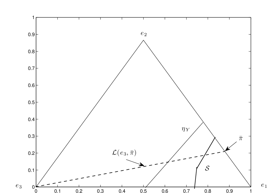
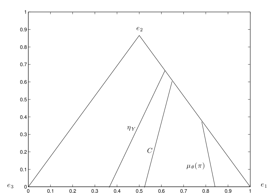
Fig.8 shows examples of a valid and invalid linear threshold. Fig.8(a) illustrates a valid MLR increasing linear threshold policy. Fig.8(b) is invalid since the threshold is less than meaning that the resulting policy is not MLR increasing on lines. Also shown is the hyperplane which by Assumption (C3) lies in polytope .

V-D2 Computation of Optimal Linear Threshold
As a consequence of Theorem 7, the optimal linear threshold approximation to threshold curve of Theorem 5 is the solution of the following constrained optimization problem:
| (54) |
where the cost is obtained as in (20) by applying threshold policy in (53).
Because the cost in (54) cannot be computed in closed form, we resort to simulation based stochastic optimization. Let denote iterations of the algorithm. The aim is to solve the following linearly constrained stochastic optimization problem:
| (55) |
Here, for each initial condition , the sample path cost is evaluated as
| (56) | ||||
A convenient way of sampling uniformly from is to use the Dirichlet distribution (i.e., , where unit exponential distribution).
The above stochastic optimization problem is solved by stochastic approximation algorithms such as the Simultaneous Perturbation Stochastic Approximation (SPSA) algorithm [47] which converges to a local minimum; see [26] for a novel parametrization that deals with the hypersphere constraints. The stochastic gradient algorithm converges to local optima, so it is necessary to try several initial conditions. The computational cost at each iteration is linear in the dimension of and is independent of the observation alphabet size . Convergence (w.p.1) can be established using techniques in [29, 30]. More sophisticated methods than SPSA can also be used. For example, [7] uses the score function method to perform gradient-based reinforcement learning. These algorithms are applicable to solve the constrained stochastic optimization problem (55). Also, if the change time distribution (specified by ) and the observation likelihoods (specified by ) are not completely specified, as long as the assumptions Theorem 5 hold, then the reinforcement learning algorithms [7] can be used to solve (55).
VI Multi-agent Quickest Time Detection with Adaptive Sensing
As mentioned in Sec.I, the social learning protocol is very similar to multi-agent quickest time detection with a sensor manager (controller). Motivated by sensor network applications, this section describes the formulation and the main results. The information patterns are similar to social learning and so the results developed in previous sections apply. The observations now can also belong to a continuum.
Consider a countable number of agents indexed by . Each agent acts once in a predetermined sequential order indexed by as follows: Based on the current belief state , agent acts as follows:
- •
Agent first chooses decision . If the agent decides to stop, then as in earlier sections, a false alarm penalty is paid, and the problem terminates.
- •
If agent chooses , then it chooses its operating mode according to a built-in micro-manager. Agent then views the world according to this mode – that is, it obtains observation from a distribution that depends on mode . It then communicates its belief state to the next agent.
Remark: An equivalent formulation is as follows: A single smart sensor adapts its operating mode at each time based on the posterior distribution of the underlying state at the previous time instant. How can quickest detection be achieved with this sensor?
How can such a network of agents, where each agent makes autonomous micro-management decisions on its mode, achieve quickest time detection? The quickest time detector can be viewed as a macro-manager that operates on the belief states and micro-manager decisions. Clearly the micro and macro-managers interact – the local decisions taken by the micro-manager determines which determines and hence determines decision of the quickest time macro-manager.
VI-A Micro-manager for Agent Mode Selection
VI-A1 Costs and mode selection
As in (8), let denote the local cost of deploying sensor mode . To avoid trivial solutions, as in Sec.IV-A, we make the submodular assumption (S).
Similar to the social learning formulation, the micro-manager picks local decision myopically as follows: Based on the belief state of the previous agent, each agent picks its mode of which sensor to deploy by minimizing its expected predicted cost:
| (57) |
where denotes the filtration . Define the convex polytopes and that partition as
| (58) |
Then from (57) it follows that for , and for , .
VI-A2 Mode dependent observations
The agent then makes an observation depending on its choice of mode . Based on its mode in (57), agent then obtains an observation from conditional probability distribution
| (59) |
Here denotes integration with respect to the Lebesgue measure (in which case and is the conditional probability density function) or counting measure (in which case is a subset of the integers and is the conditional probability mass function ). The key point is that unlike classical quickest detection, each agent now views the world based on its selected mode .
Let denote the belief state update if mode is chosen and measurement obtained. It is given by the HMM filter (7) with mode dependent probabilities . That is,
| (60) |

VI-B Macro-Manager for Quickest Time Detection
Below we present the assumptions and main result. Based on the above micro-manager protocol, the aim is to perform quickest time change detection. So the quickest detection problem can be viewed as optimizing the cost function (24) subject to the constraint that the belief state evolves according to (60). The setup is identical to that in Sec.II-B and Sec.III-A. For , agents choose and at , agent picks . The optimal policy of the macro-manager satisfies Bellman’s equation (25).
The following theorems mimic the results for the social learning based quickest detection problem, and their proofs are identical.
VI-B1 Blackwell Dominance
Suppose the mode dependent observation matrices are of the form where and , are stochastic kernels. Then an identical proof to Theorem 1 shows that classical quickest detection with observation matrix always yields a lower cost than mode dependent quickest detection with observation matrices , where the mode is chosen according to any arbitrary strategy.
VI-B2 Threshold Policies
Consider the following assumptions that are similar to (C1) in Sec.V-A and (C2) in Sec.V-B. Recall vertices are defined in (45) and denote vertices of hyperplane .
- (C1)
If lies in one of the polytopes , then , for all .
- (C2)
, , .
We have the following result regarding the structure of for quickest time detection.
Theorem 8.
(C1) and (C2) are relatively easy to check even if is continuum as shown below. For all , let denote the maximum support of the distribution , i.e., .
Lemma 4.
(C1), (C2) hold if their inequalities hold for .
Thus only a finite number of inequalities need to be verified. In particular for a Gaussian distribution, since , the filter becomes the Bayesian predictor . So it suffices to check that for (C1) to hold.
Proof.
Consider (C1). is equivalent to verifying since is non-negative for all . So we need to check that for all . But since and are TP2 according to Assumptions (A1), (A2), from Theorem 10(4) in Appendix A-F, the belief state update is MLR increasing in . Moreover by (A3) has decreasing elements. Therefore from Result 1 in Appendix A-A, is decreasing in . So it suffices to check that .
VII Numerical Results
In addition to the numerical examples presented earlier, this section presents two numerical examples. The first example illustrates the multiple threshold policies inherent in social learning (this example was mentioned in Sec.I). The second example illustrates the optimal threshold curve for a PH-type distributed change time that was proved in Theorem 5.
Example 1. Geometric Distributed Change Time: This examples illustrates the existence of a triple threshold policy for quickest time change detection when the change time is geometrically distributed. We chose the social learning model with parameters (so is a one dimensional simplex), , ,
For the global quickest time detection parameters we chose , delay , false alarm vector (i.e., ). It is easily checked that (A1), (A2) and (S) hold.
The optimal policy is shown in Fig.1(a) and comprises of a triple threshold policy. It was computed by constructing a uniform grid of 500 points for and then implementing the value iteration algorithm (27) for a horizon of . The ‘x’ in Fig.1(a) and (b) are the values of , and , respectively.
Example 2. Phase Distributed Change Time: This examples illustrates Theorem 5 which proved the existence of a single threshold curve for social learning based quickest time change detection with PH-distributed change time. We model the PH-distribution via a 3-state Markov chain. So the belief space is a two dimensional simplex (equilateral triangle) and can be visualized easily.
We chose the social learning model with parameters , . The observation probabilities and local decision costs were chosen as
The PH-distributed change times were modelled by the 3 state Markov chain with transition probability . To illustrate the quickest time detection, we chose 4 candidate transition probability matrices, namely,
Note models the geometric distribution since states 2 and 3 are indistinguishable – in fact it is exactly lumpable [24] into the 2 state Markov chain with transition matrix .
Fig.10 plots the probability mass function (see (4)) of the PH-distributed change time for these four transition matrices for . Fig.10 shows these PH-distributions are quite different in behavior to a geometric distribution – they are non-monotone and have heavier tails.

It is easily checked that (A1), (A2), (A3), (S), (PH), (C2) and (C3) of Theorem 5 hold. Fig.11 shows the optimal decision policies for these four cases with the stopping set shaded. The optimal policy was computed as follows. A grid of values was formed within the 2-dimensional unit simplex .Then the value iteration algorithm (27) was solved for horizon (in all cases implying that the value iteration algorithm converged). In all 4 cases, the optimal decision policy is characterized by a single threshold curve in polytope . This is consistent with Theorem 5.
In each plot of Fig.11 also shows the hyperplanes (defined in (24)) and (defined in (35). The polytope is to the right of hyperplane . The remaining line segments from left to right are . Note that hyperplane lies in , thereby satisfying Assumption (PH) and (C3).
Actually cases and satisfy Assumptions (C1), and (PH) and so Theorem 4 holds. Therefore, for these two cases, the optimal threshold curve is the linear hyperplane as can be seen in Fig.11.


VIII Conclusions
Motivated by understanding how local and global decision making interact, this paper has presented structural results for quickest time detection when agents perform social learning. Also a related model incorporating multi-agent sensor scheduling and quickest time detection was considered. Unlike classical quickest detection, the optimal policy can have multiple thresholds. Four main results were presented. First, Theorem 1 showed using Blackwell dominance of measures that social learning based quickest detection always results in more expensive cost compared to classical quickest detection. Second, for symmetric observation probabilities and geometric change times, the explicit multi-threshold behavior of social learning based quickest detection was characterized in Theorem 3 by approximating with a simpler detection problem. Third, quickest time change detection for more general PH-type distributed change times was considered. Theorem 4 gave sufficient conditions for the optimal policy to be characterized by a single linear hyperplane in the multi-dimensional simplex of posterior distributions. Finally, using lattice programming and likelihood ratio dominance Theorem 5 gave sufficient conditions for the optimal policy to be characterized by a single switching curve. The optimal linear approximation to this curve (that preserves the MLR monotone nature of the policy) was characterized in Theorem 7.
The results of this paper are straightforwardly extended to more general stopping problems where the underlying Markov state does not have an absorbing state, as long as the transition matrix satisfies assumption (A2). In current work, we are using similar social learning models for “order-book” trades in agent based models for algorithmic market making, see also [38].
Appendix A Proofs of Theorems
A-A Preliminaries: Stochastic Dominance, Submodularity
Excellent background references for stochastic dominance and lattice programming are [49, 25, 35, 23]. The proofs of Theorem 2 and Theorem 5 require concepts in stochastic dominance. In particular, Statement (iv) of Theorem 5 states that the optimal social policy is monotonically increasing in belief state . In order to compare belief states and , we will use the monotone likelihood ratio (MLR) stochastic ordering and a specialized version of the MLR order restricted to lines in the simplex . The MLR order is useful for social learning since it is preserved after conditioning [40, 23, 35].
Definition 1 (MLR ordering, [35, pp.12–15]).
Let be any two belief state vectors. Then is greater than with respect to the MLR ordering – denoted as , if
| (61) |
Definition 2 (First order stochastic dominance).
Let . Then first order stochastically dominates – denoted as – if for .
Result 1 ([35]).
(i) implies . (For , and are equivalent)
(ii) Let denote the set of all dimensional vectors
with
nondecreasing components, i.e., .
Then iff for all ,
.
(iii) Suppose , and are increasing in . Then implies .
(This follows since from (ii) and since ).
For state-space dimension , MLR is a complete order and coincides with first order stochastic dominance. For state-space dimension , MLR is a partial order, i.e., is a partially ordered set (poset) since it is not always possible to order any two belief states .
Finally, we define a modification of the MLR order on certain line segments in the simplex which yields a total ordering.
Define the set of belief states . For each belief state , denote the line segment that connects to . Thus
| (62) |
Definition 3 (MLR ordering and on lines).
is greater than with respect to the MLR ordering on the line – denoted as if for some and . Similarly, , if ) for some , and .
Note that is a chain, i.e., all elements are comparable, i.e., either or . Similarly is a chain. In Lemma 5, we summarize useful properties of that will be used in our proofs.
Lemma 5.
Consider
, .
(i) On , is the least and is the greatest element.
On , is the least and is the greatest.
(ii) Convex combinations of MLR comparable belief states form a chain.
For any ,
.
(iii) All points on a line
are MLR comparable. Consider any two points
(62) where
.
Then
, implies . A similar result holds for .
Definition 4 (Submodular function [49]).
is submodular (antitone differences) if , for , .
The following result says that for a submodular function , is increasing in its argument . This implies is MLR increasing on the line segments , which in turn will be used to prove the existence of as threshold decision curve.
Theorem 9 ([49]).
If is submodular, then
there exists a
, that is increasing on
,
i.e., .
Definition 5 (Single Crossing Condition [49, 4]).
satisfies a single crossing condition in if implies for and . Then is increasing in .
Definition 6 (TP2 ordering and Reflexive TP2 distributions).
Let and
denote any two multivariate probability mass functions.
Then:
(i) if .
If and are univariate, then this definition is equivalent to
the MLR ordering defined above.
(ii) A multivariate
distribution is said to be multivariate TP2 if holds,
i.e., .
(iii) If
are scalar indices,
Statement (ii) is equivalent to saying that a matrix is TP2 if all
second order minors are non-negative. if , then the -th row of MLR dominates the
-th row.
A-B Proof of Theorem 1
Let denote the value function at iteration of the value iteration algorithm (27) associated with the classical quickest detection Bellman equation (29). Recall is the value function associated with the social learning based quickest detection problem (25).
We start with the following lemma which is proved at the end of Appendix A-B
Lemma 6.
.
The proof of Theorem 1 then follows by mathematical induction using the value iteration algorithm (27). Assume for . Then
where the second inequality follows from Lemma 6. Thus . This completes the induction step. Since value iteration converges pointwise, thus proving the theorem.
Proof of Lemma 6.
Step 1: First, let us show that is concave over for any by induction.
Recall from (27) that which is linear in .
Assume is concave at iteration . Note that is positively homogeneous, i.e.,
for any , . So the value iteration algorithm (27) associated with Bellman’s
equation (29) is
Since the composition of concave function with a linear function preserves concavity, therefore is concave and so is concave.
A-C Proof of Theorem 2
Theorem 2 (Detailed version).
Under (A1), (A2), (S),
(i) The local decision (see (9)) is increasing in .
(ii) is
MLR increasing in , i.e., .
(iii) The linear hyperplanes , do not intersect
within the interior of the belief space . Thus, out of the polytopes in (30),
there are a maximum of non-empty polytopes in , namely (31).
(iv) Let . Then
each of the hyperplanes , partitions
such that the vertices lie in the convex polytope
and the vertices lie in the convex polytope
.
(v)
decreases with .
(vi) defined in (13) has the following structure:
| (63) |
Proof: (i) From [33, Lemma1.2(1)] if and are TP2 (i.e., (A1), (A2) hold) then . Next MLR dominance implies first order stochastic dominance. Then since from (S), is increasing in , it follows that . Since the denominators are non-negative, this implies that . That is, the single crossing condition (36) holds, see Definition 5. So .
(ii) To prove wrt , we use a similar approach to Part (i). From [33, Lemma 1.2(2)], assuming (A3), implies . As in the proof above, using (S) this implies . Since the denominators are non-negative, this implies that
| (64) |
That is a single crossing condition (see Definition 5) holds wrt and the partial order . So .
(iii) follows immediately from (36).
(iv) Since , clearly . Next since , the single crossing condition (64) yields .
(v) Start with the single crossing condition (36) repeated below for clarity:
(vi) follows by enumerating all matrices that satisfy (i) and (ii); see (33) for an example.
A-D Proof of Theorem 3
Similar to the example given below Theorem 2, it can be verified from (13) that there are only 3 possible values for , namely,
| (65) |
Thus Bellman’s equation (25), reads
| (66) |
Claim (i): For , . This can be solved explicitly as
Since is MLR decreasing in , the optimal policy for is a threshold policy
with threshold at . This proves the first claim of the theorem.
Claim (ii) Since for , the private belief state update
(7)
freezes in these regions,
i.e., implies
that , .
Therefore all agents take the same local decision according to (9) implying an information cascade.
Claim (iii) The proof of this is more involved.
We need the following property of the social learning Bayesian filter which is a detailed version of Lemma 2 in Sec.IV-B. Since we are going to partition into four intervals, namely , , and , it is convenient to introduce the following notation: Denote these intervals as , respectively. Note , , .
Lemma 2 (Detailed version).
Consider the social learning Bayesian filter (11).
Then
, . Furthermore if is symmetric TP2, then
, and .
So
(i) implies and
.
(ii) implies and
.
The proof of Lemma 2 is as follows. Recall from (65) that on interval , . Then it is straightforwardly verified from (11) that . Next, using (11) it follows that is a sufficient condition for and . Also, since by (A1) is TP2, applying Theorem 10(2), implies . So symmetric TP2 is sufficient for the claims of the lemma to hold. Statements (i) and (ii) then follow straightforwardly. In particular, from Theorem 10(1), implies , which implies Statement (i) of the lemma. Statement (ii) follows similarly.
Returning to the proof of Theorem 3, we use mathematical induction on the value iteration algorithm (27). Clearly is linear. Assume now that is piecewise linear and concave on each of the four intervals . That is, for two dimensional vectors in the set ,
Consider . From (65), since , , Lemma 2 (i) together with the value iteration algorithm (66) yields
Note the crucial point in the above equation: as a result of Lemma 2 (i) – the social learning filter maps to only (for ) and (for ). Since each of the terms in the above equation are piecewise linear and concave, it follows that is piecewise linear and concave on . A similar proof holds for and this involves using Lemma 2(ii). As a result the stopping set on each interval , is a convex region, i.e., an interval. This proves claim (ii).
A-E Proof of Lemma 3 and Theorem 4
Proof of Lemma 3
Let us introduce the following notation. Define
| (67) |
The proof comprises of three parts.
Statement (i): Under (PH), for every , there exists a such that
.
Proof:
Consider any belief state .
Construct a line segment from through the belief state and let this line segment intersect the hyperplane .
Denote as this point of intersection.
Clearly where . It is straightforwardly established
that if which is clearly true since and for .
Statement (ii): Under (A1), (A2), (A3), if , then
.
Proof:
Under (A1), (A2), (A3), it follows from Theorem 10(2) in Appendix A-F that is MLR increasing, that is, implies .
Under (A3), the elements of are decreasing.
So from Result 1 in Appendix A-A, it follows that
.
So
implies
.
Statements (i) and (ii) imply that if the social learning filter (11) maps belief states in to , then all belief states in are also mapped to .
Since the hyperplane has infinite points, how can we formulate a sufficient
condition for belief states to be mapped to the polytope ?
(C1) serves as a sufficient condition as proved in Statement (iii) below.
Statement (iii): A sufficient condition for to hold for all is that
for all vertices of (45).
Proof: Clearly every belief state is a convex combination of the vertices, i.e.,
, for some and . Now
is equivalent to since the normalization term in is
non-negative.
This implies , and this is equivalent
to .
Proof of Theorem 4
Define .
Step 1: We first prove that for . This is equivalent to saying
that for , the optimal policy .
The proof of Step 1 is by induction on the value iteration algorithm (27). Suppose . Then it trivially satisfies for . Next suppose for . Then for , Assumption (C1) implies that belongs to implying that . So from (27), it follows that since for . Since converges pointwise to , Step 1 follows. For initial condition (see (27)), obtained as the limit of the value iteration algorithm is identical to that with initial condition .
Step 2: From Bellman’s equation it follows trivially that for , .
From Steps 1 and 2, we have iff .
A-F Proof of Theorem 5
This section is in two parts. We start with several preliminary results that are similar to the results in [33]. Then the proof of Theorem 5 is presented.
A-F1 Structural Properties of Social Learning Filter
Theorem 10.
The following structural properties hold for the public belief update evaluated by the social learning Bayesian filter defined in (11):
- 1.
Under (S), is TP2 for , see Definition 6.
- 2.
Under (A1), (A2), (S) if , then implies
- 3.
Under (A1), (A2), (S), if , then .
- 4.
Under (A1), (A2), if , then implies .
Proof.
1). We need to show that for fixed ,
| (68) |
Recall from (13) that is a matrix with a single 1 in each row at and all other elements zero. So the only non trivial case to prove is when both terms on the LHS are 1, i.e., and . Assuming (A2), (S), Theorem 2(i) says that . This means that and . In either case (68) holds with equality since the RHS is identical to the LHS.
2). Since is TP2 (A2), we have for , see [23]. So it suffices to show that for . Moreover, since belong to the same polytope , (say), see (30). From [23], a sufficient condition for is that is TP2. Of course we need this to hold on each of the polytopes, i..e, for .
So under what conditions is TP2 in each of the polytopes? Note (A2) says is TP2. Since (see (13)) and the product of TP2 matrices is TP2 [23, pp.471], it only remains to prove that is TP2. This follows from (S) as proved in (i) above.
3). Since is TP2 (A2), it suffices to prove that implies , i.e., . From Statement 1, and are TP2 and from (A2) is TP2. So and are TP2. Therefore, from Definition 6(iii), the rows of and are MLR increasing. Since MLR dominance implies first order stochastic dominance, this means that both and are increasing with . Since , Result 1(i),(ii) and (iii), imply that a sufficient condition for is that or equivalently, . A sufficient condition for this is . But this condition holds from the structure of in (63) and the fact that is MLR increasing wrt (Statement (ii) of Theorem 2 in Appendix A-C).
4). Since is TP2 (A2), it suffices to prove that for . Since is TP2 (A1), this result follows straightforwardly from [51, Theorem 4].
A-F2 Proof of Theorem 5
Here we prove Theorem 5. The update of belief state in is simple, since (uniformly distributed) for each , see (34) for example. In comparison, the sensor management case of Theorem 8 on with update given by (60) requires an arbitrary TP2 matrix . To allow for this generality, in the proof below, we assume is an arbitrary TP2 matrix on .
Part 1: Under (A1), (A2), (A3), (S), (C3), (C2), (PH), is MLR decreasing on polytope :
The proof of Part 1 is by mathematical induction on the value iteration algorithm (27). Start
with
in (27). Clearly this is MLR decreasing on and therefore on polytope since
is chosen with increasing elements, see (17).
Now for the inductive step: Assume at iteration , is MLR decreasing on polytope .
Then since is MLR increasing in (Theorem 10(4)) and by (C2), it follows that
.
Consider any . Since (see Theorem 10(3)),
| (69) |
Next since (Theorem 10(2)), so MLR decreasing in implies . So from (69), implies
| (70) |
From (A3), is MLR decreasing. So implies . Therefore implies . Thus , i.e., . This completes the induction step. Finally, since as pointwise (see discussion below (27)), is MLR decreasing on polytope .
Part 2: Under the above conditions, is MLR increasing on polytope . It suffices to show that is submodular (see Definition 4) on wrt the MLR ordering since then Theorem 9 applies implying that is MLR decreasing in . To show that in (25) is submodular, we need to show that is MLR decreasing in . But this follows from (A3) and Part 1. Thus from Theorem 9, (49) holds.
A-G Proof of Theorem 7
Given any with , we need to prove: iff , for . But from the structure of (53), obviously is equivalent to , or equivalently, .
Now from Lemma 5(iii), implies that , and . Substituting these into the above expression, we need to prove
iff , , . This is obviously true.
A similar proof shows that on lines the linear threshold policy satisfies iff for .
References
- [1] D. Acemoglu and A. Ozdaglar. Opinion dynamics and learning in social networks. Dynamic Games and Applications, pages 1–47, 2010.
- [2] D. Acemoglu, A. Ozdaglar, and A. Tahbaz-Salehi. Cascades in networks and aggregate volatility. Technical report, National Bureau of Economic Research, 2010.
- [3] I. F. Akyildiz, W. Su, Y. Sankarasubramaniam, and E. Cayirci. Wireless sensor networks: A survey. Computer Networks, 38(4):393–422, 2002.
- [4] R. Amir. Supermodularity and complementarity in economics: An elementary survey. Southern Economic Journal, 71(3):636–660, 2005.
- [5] M.S. Andersland and D. Teneketzis. Measurement scheduling for recursive team estimation. Journal of Optimization Theory and Applications, 89(3):615–636, June 1996.
- [6] A. Banerjee. A simple model of herd behavior. Quaterly Journal of Economics, 107:797–817, 1992.
- [7] P. Bartlett and J. Baxter. Estimation and approximation bounds for gradient-based reinforcement learning. J. Comput. Syst. Sci., 64(1):133–150, 2002.
- [8] M. Basseville and I.V. Nikiforov. Detection of Abrupt Changes — Theory and Applications. Information and System Sciences Series. Prentice Hall, New Jersey, USA, 1993.
- [9] D.P. Bertsekas. Dynamic Programming and Optimal Control, volume 1 and 2. Athena Scientific, Belmont, Massachusetts, 2000.
- [10] S. Bikchandani, D. Hirshleifer, and I. Welch. A theory of fads, fashion, custom, and cultural change as information cascades. Journal of Political Economy, 100:992–1026, 1992.
- [11] L. Bru and X. Vives. Informational externalities, herding, and incentives. Journal of Institutional and Theoretical Economics JITE, 158(1):91–105, 2002.
- [12] C. Chamley. Rational herds: Economic models of social learning. Cambridge, 2004.
- [13] C. Chamley and D. Gale. Information revelation and strategic delay in a model of investment. Econometrica, 62(5):1065–1085, 1994.
- [14] Y. Chen, Q. Zhao, V. Krishnamurthy, and D. Djonin. Transmission scheduling for optimizing sensor network lifetime: A stochastic shortest path approach. IEEE Trans. Signal Proc., 55(5):2294–2309, May 2007.
- [15] T. Cover and M. Hellman. The two-armed-bandit problem with time-invariant finite memory. Information Theory, IEEE Transactions on, 16(2):185–195, 1970.
- [16] F.R. Gantmacher. Matrix Theory, volume 2. Chelsea Publishing Company, New York, 1960.
- [17] S. Hart. Adaptive heuristics. Econometrica, 73(5):1401–1430, 2005.
- [18] S. Hart and A. Mas-Colell. A simple adaptive procedure leading to correlated equilibrium. Econometrica, 68(5):1127–1150, 2000.
- [19] M.E. Hellman and T.M. Cover. Learning with finite memory. The Annals of Mathematical Statistics, pages 765–782, 1970.
- [20] O. Hernández-Lerma and J. Bernard Laserre. Discrete-Time Markov Control Processes: Basic Optimality Criteria. Springer-Verlag, New York, 1996.
- [21] D.P. Heyman and M.J. Sobel. Stochastic Models in Operations Research, volume 2. McGraw-Hill, 1984.
- [22] S. Karlin. Total Positivity, volume 1. Stanford Univ., 1968.
- [23] S. Karlin and Y. Rinott. Classes of orderings of measures and related correlation inequalities. I. Multivariate totally positive distributions. Journal of Multivariate Analysis, 10:467–498, 1980.
- [24] J.G. Kemeny and J.L. Snell. Finite Markov Chains. Van Nostrand, New York, 1960.
- [25] M. Kijima. Markov Processes for Stochastic Modelling. Chapman and Hall, 1997.
- [26] V. Krishnamurthy. Bayesian sequential detection with phase-distributed change time and nonlinear penalty – a lattice programming pomdp approach. IEEE Trans. Inform. Theory, 57(3), Oct. 2011. http://arxiv.org/abs/1011.5298.
- [27] V. Krishnamurthy, M. Maskery, and G. Yin. Decentralized activation in a ZigBee-enabled unattended ground sensor network: A correlated equilibrium game theoretic analysis. IEEE Trans. Signal Proc., 56(12):6086–6101, December 2008.
- [28] V. Krishnamurthy and B. Wahlberg. POMDP multiarmed bandits – structural results. Mathematics of Operations Research, 34(2):287–302, May 2009.
- [29] V. Krishnamurthy and G. Yin. Recursive algorithms for estimation of hidden Markov models and autoregressive models with Markov regime. IEEE Trans. Inform. Theory, 48(2):458–476, February 2002.
- [30] H.J. Kushner and G. Yin. Stochastic Approximation Algorithms and Recursive Algorithms and Applications. Springer-Verlag, 2nd edition, 2003.
- [31] I. Lobel, D. Acemoglu, M. Dahleh, and A.E. Ozdaglar. Preliminary results on social learning with partial observations. In Proceedings of the 2nd International Conference on Performance Evaluation Methodolgies and Tools, Nantes, France, 2007. ACM.
- [32] W.S. Lovejoy. On the convexity of policy regions in partially observed systems. Operations Research, 35(4):619–621, July-August 1987.
- [33] W.S. Lovejoy. Some monotonicity results for partially observed Markov decision processes. Operations Research, 35(5):736–743, Sept.-Oct. 1987.
- [34] G.B. Moustakides. Optimal stopping times for detecting changes in distributions. Annals of Statistics, 14:1379–1387, 1986.
- [35] A. Muller and D. Stoyan. Comparison Methods for Stochastic Models and Risk. Wiley, 2002.
- [36] M.F. Neuts. Structured stochastic matrices of M/G/1 type and their applications. Marcel Dekker, N.Y., 1989.
- [37] J. Papastravrou, J. Pothiawala, and M. Athans. Designing an organization in a hypothesis testing framework. Technical report, Laboratory for Information and Decision Systems, MIT, 1989.
- [38] A. Park and H. Sabourian. Herding and contrarian behavior in financial markets. Econometrica, 79(4):973–1026, 2011.
- [39] H.V. Poor and O. Hadjiliadis. Quickest Detection. Cambridge, 2008.
- [40] U. Rieder. Structural results for partially observed control models. Methods and Models of Operations Research, 35:473–490, 1991.
- [41] S. Ross. Introduction to Stochastic Dynamic Programming. Academic Press, San Diego, California., 1983.
- [42] S. Ross, M. Izadi, M. Mercer, and D. Buckeridge. Sensitivity analysis of POMDP value functions. In IEEE International Conference on Machine Learning and Applications ICMLA’09, 2009.
- [43] AN Shiryaev. On optimum methods in quickest detection problems. Theory of Probability and its Applications, 8:22, 1963.
- [44] A.N. Shiryayev. Optimal stopping rules. Springer-Verlag, 1978.
- [45] L. Smith and P. Sorensen. Informational herding and optimal experimentation. Economics Papers 139, Economics Group, Nuffield College, University of Oxford, 1997.
- [46] L. Smith and P. Sorenson. Pathological outcomes of observational learning. Econometrica, 68(2):371–398, 2000.
- [47] J. Spall. Introduction to Stochastic Search and Optimization. Wiley, 2003.
- [48] A.G. Tartakovsky and V.V. Veeravalli. General asymptotic Bayesian theory of quickest change detection. Theory of Probability and its Applications, 49(3):458–497, 2005.
- [49] D.M. Topkis. Supermodularity and Complementarity. Princeton University Press, 1998.
- [50] CC White and DP Harrington. Application of Jensen’s inequality to adaptive suboptimal design. Journal of Optimization Theory and Applications, 32(1):89–99, 1980.
- [51] W. Whitt. A note on the influence of the sample on the posterior distribution. Journal American Statistical Association, 74:424–426, 1979.
- [52] B. Yakir. A note on optimal detection of a change point in distribution. Annals of Statistics, 25:2117–2126, 1997.
- [53] B. Yakir, A.M. Krieger, and M. Pollak. Detecting a change in regression: First-order optimality. Annals of Statistics, 27(6):1896–1913, 1999.
| Vikram Krishnamurthy (S’90-M’91-SM’99-F’05) was born in 1966. He received his bachelor’s degree from the University of Auckland, New Zealand in 1988, and Ph.D. from the Australian National University in 1992. He currently is a professor and Canada Research Chair at the Department of Electrical Engineering, University of British Columbia, Vancouver, Canada. Dr Krishnamurthy’s current research interests include computational game theory, stochastic control in sensor networks, and stochastic dynamical systems for modeling of biological ion channels and biosensors. Dr. Krishnamurthy currently serves as Editor in Chief of IEEE Journal Selected Topics in Signal Processing. He has served as associate editor for several journals including IEEE Transactions Automatic Control and IEEE Transactions on Signal Processing. In 2009-2010, he served as Distinguished lecturer for the IEEE signal processing society. |