跳到论文正文
W Papers独立论文阅读器 arXiv:1007.0398 论文正文 计算阅读时间 · 0%
引用这篇论文根据当前论文元数据生成,正式投稿前建议核对。


License: arXiv.org perpetual non-exclusive license
arXiv:1007.0398v1 [math.SP] 02 Jul 2010

On δ′\delta^{\prime}-like potential scattering on star graphs

S S Man’ko Affiliation: Department of Mechanics and Mathematics, Ivan Franko National University of Lviv, 1 Universytetska str., 79000 Lviv, Ukraine Email: s_ manko@franko.lviv.ua
Abstract

We discuss the potential scattering on the noncompact star graph. The Schrödinger operator with the short-range potential localizing in a neighborhood of the graph vertex is considered. We study the asymptotic behavior the corresponding scattering matrix in the zero-range limit. It has been known for a long time that in dimension 1 there is no non-trivial Hamiltonian with the distributional potential δ′\delta^{\prime}, i.e., the δ′\delta^{\prime} potential acts as a totally reflecting wall. Several authors have, in recent years, studied the scattering properties of the regularizing potentials α​ε−2​Q​(x/ε)\alpha\varepsilon^{-2}Q(x/\varepsilon) approximating the first derivative of the Dirac delta function. A non-zero transmission through the regularized potential has been shown to exist as ε→0\varepsilon\to 0. We extend these results to star graphs with the point interaction, which is an analogue of δ′\delta^{\prime} potential on the line. We prove that generically such a potential on the graph is opaque. We also show that there exists a countable set of resonant intensities for which a partial transmission through the potential occurs. This set of resonances is referred to as the resonant set and is determined as the spectrum of an auxiliary Sturm-Liouville problem associated with QQ on the graph.

pacs
02.30.Tb, 03.65.Nk, 02.30.Hq

1 Introduction

Schrödinger operators with potentials supported on a discrete set of points (such potentials are usually termed “point interactions”) have attracted considerable attention both in the physical and mathematical literature over several past decades. One of the reasons for this is that such singular Hamiltonians are widely used in various application to atomic, nuclear, and solid state physics. Applications also arise in optics, for instance, in dielectric media where electromagnetic waves scatter at boundaries or thin layers. Another reason is that Schrödinger operators with point interactions often form “solvable” models in the sense that the resolvents of such operators can explicitly be calculated. Consequently the spectrum, the eigenfunctions, as well as resonances and scattering quantities, can also be determined explicitly (see [2, 3] and references therein). In the physically oriented literature point interactions are often understood as sharply localized potentials, exhibiting a number of interesting features and unusual effects not seen for regular potentials.

Currently, there is increasing interest in solvable models on graphs in particular, as a reaction to a great deal of progress in fabricating graph-like structures of a semiconductor material, for which graph Hamiltonians represent a natural model (see the survey [20] for details). The idea to investigate quantum mechanics of particles confined to a graph originated with the study of free electron models of organic molecules [24, 25, 26]. Among the systems that were successfully modeled by quantum graphs we mention e.g., single-mode acoustic and electro-magnetic waveguide networks [14], Anderson transition [4] and quantum Hall systems with long range potential [6], fracton excitations in fractal structures [5], and mesoscopic quantum systems [19]. The essential component of such graph models is the wavefunction coupling in the vertices. The interface conditions have to be chosen to make the Hamiltonian self-adjoint, or in physical terms, to ensure conservation of the probability current at the vertex.

One of the most natural way to define a graph Hamiltonian corresponding to a point interaction supported by the branching point is to choose an appropriate self-adjoint extension of the corresponding free Hamiltonian with the interactions points removed. This approach has been realized in [13], where the authors found that a vertex joining nn graph edges can be described by n2n^{2} real parameters defining the interface condition at the vertex. A general form of such a coupling was described in [18] by a pair of n×nn\times n matrices A\mathrm{A}, B\mathrm{B} such that rank(A,B)=n\mathop{\rm rank}{(\mathrm{A},\mathrm{B})}=n and AB∗\mathrm{AB}^{*} is self-adjoint; the boundary values have to satisfy the conditions

A​Ψ​(a)+B​Ψ′​(a)=0.\mathrm{A}\Psi(a)+\mathrm{B}\Psi^{\prime}(a)=0. (1)

Here the symbol Ψ⁡(a)\Psi(a) is used for the column vector of the boundary values at the vertex aa, and analogously Ψ′​(a)\Psi^{\prime}(a) stands for the vector of the first derivatives, taken all in the outgoing direction.

Another possible approach to define the vertex coupling is to approximate a quantum graph with a thin quantum waveguide (see [1, 23, 8, 12] and references therein). Different vertex couplings were also discovered in [10, 11, 13, 7].

The Schrödinger operators with the Dirac delta-function and its derivatives in potentials have been studying intensively since the eighties of last century (see [2, 3, 9] and the references given there). One of the first well-studied Hamiltonian was the operator with Dirac’s delta-function potential δ\delta. A case of special interest arises when the δ\delta-potential is replaced by the derivative δ′\delta^{\prime} of the Dirac delta-function. Šeba [27] appears to have been among the first to consider such a Hamiltonian. To define the Hamiltonian −d2d​x2+δ′​(x)-\frac{d^{2}}{dx^{2}}+\delta^{\prime}(x) he approximated δ′\delta^{\prime} by regular potentials ε−2​Q​(x/ε)\varepsilon^{-2}Q(x/\varepsilon) and then investigated the convergence of the corresponding family of regular Schrödinger operators

Sε=−d2d​x2+1ε2​Q​(xε).\mathrm{S}_{\varepsilon}=-\frac{d^{2}}{dx^{2}}+\frac{1}{\varepsilon^{2}}Q\Bigl(\frac{x}{\varepsilon}\Bigr).

Here QQ is an integrable function. If QQ has zero mean and the integral ∫ℝt​Q​(t)​𝑑t\int_{\mathbb{R}}t\,Q(t)\,dt is equal to −1-1, then the sequence ε−2​Q​(x/ε)\varepsilon^{-2}Q(x/\varepsilon) converges in the sense of distributions as ε→0\varepsilon\to 0 to δ′\delta^{\prime}, which served as motivation for such an approximation. Šeba claimed that the operators Sε\mathrm{S}_{\varepsilon} converge in the uniform resolvent sense to the direct sum of the unperturbed half-line Schrödinger operators subject to the Dirichlet boundary conditions at x=0x=0. From the viewpoint of scattering theory it means that the δ′\delta^{\prime}-barrier is completely opaque, i.e., in the limit ε→0\varepsilon\to 0 the potential ε−2​Q​(x/ε)\varepsilon^{-2}Q(x/\varepsilon) becomes a totally reflecting wall at x=0x=0 splitting the system into two independent subsystems lying on the half-lines (−∞,0)(-\infty,0) and (0,∞)(0,\infty).

But this result is in conflict with conclusions reached in [28], where the resonances in the transmission probability for δ′\delta^{\prime}-like potential have been observed. In that paper an exactly solvable model with a step function α​Q\alpha Q was considered. The authors found a discrete set of intensities αn\alpha_{n}, for which partial transmission through the limiting δ′\delta^{\prime}-potential occurs. The values αn\alpha_{n} are roots of a transcendent equation depending on the regularization QQ. Exactly solvable models with other piecewise constant potentials as well as nonrectangular regularizations of δ′\delta^{\prime} have later been studied in [29, 30, 31, 32] and the same conclusion has been drawn.

In [15, 16] the authors approximated the formal Hamiltonian −d2d​x2+q⁡(x)+α​δ′​(x)-\frac{d^{2}}{dx^{2}}+q(x)+\alpha\delta^{\prime}(x) on the line by regular Schrödinger operators

Sε​(α,Q)=−d2d​x2+q⁡(x)+αε2​Q​(xε)\mathrm{S}_{\varepsilon}(\alpha,Q)=-\frac{d^{2}}{dx^{2}}+q(x)+\frac{\alpha}{\varepsilon^{2}}Q\Bigl(\frac{x}{\varepsilon}\Bigr)

and the similar resonant effect was discovered. Here the function Q∈C0∞​(−1,1)Q\in C_{0}^{\infty}(-1,1) has zero mean, α\alpha is a real coupling constant, and qq is a real valued fixed potential tending to +∞+\infty as |x|→∞|x|\to\infty, which ensures that the spectrum of Sε​(α,Q)\mathrm{S}_{\varepsilon}(\alpha,Q) is discrete. The map assigning a selfadjoint operator S⁡(α,Q)\mathrm{S}(\alpha,Q) to each pair (α,Q)(\alpha,Q) was constructed there. The choice of S⁡(α,Q)\mathrm{S}(\alpha,Q) was determined by proximity of its energy levels and pure states to those for the Hamiltonian with regularized potentials for small ε\varepsilon. It was established that for almost all coupling constants the operator S⁡(α,Q)\mathrm{S}(\alpha,Q) is just the direct sum of the Schrödinger operators with potential qq on half-axes subject to the Dirichlet boundary conditions at the origin. But in the exceptional case the nontrivial coupling at the origin arises. The notion of the resonant set ΣQ\Sigma_{Q}, which is the spectrum of the problem

−g′′+α​Q​(t)​g=0,t∈(−1,1),g′​(−1)=g′​(1)=0,-g^{\prime\prime}+\alpha Q(t)g=0,\quad t\in(-1,1),\qquad g^{\prime}(-1)=g^{\prime}(1)=0,

with respect to the spectral parameter α\alpha was introduced in [15, 16]. It was also constructed the coupling function θQ:ΣQ→ℝ\theta_{Q}:\,\Sigma_{Q}\to\mathbb{R} defined via θQ​(α)=gα​(1)/gα​(−1)\theta_{Q}(\alpha)=g_{\alpha}(1)/g_{\alpha}(-1), where gαg_{\alpha} is an eigenfunction corresponding to the eigenvalue α∈ΣQ\alpha\in\Sigma_{Q}. In the case when the coupling constant α\alpha belongs to the resonance set, the δ′\delta^{\prime}-barrier admits a partial transmission of a particle, and an appropriate wave function obeys the interface conditions

ψ⁡(+0)=θQ​(α)​ψ​(−0),θQ​(α)​ψ′​(+0)=ψ′​(−0).\psi(+0)=\theta_{Q}(\alpha)\psi(-0),\qquad\theta_{Q}(\alpha)\psi^{\prime}(+0)=\psi^{\prime}(-0).

Studies of [15, 16] have been continued in [17, 21]. First the findings of [28, 29, 30, 31, 32] were generalized in [21], where the scattering on an arbitrary potential of the form α​ε−2​Q​(x/ε)\alpha\varepsilon^{-2}Q(x/\varepsilon) has been considered. It was proved that such a potential is asymptotically transparent only if a coupling constant belongs to the resonant set. Moreover, the scattering amplitude for the Hamiltonians Sε​(α,Q)\mathrm{S}_{\varepsilon}(\alpha,Q) and −d2d​x2-\frac{d^{2}}{dx^{2}} converges as ε→0\varepsilon\to 0 to that for the limiting Hamiltonian S⁡(α,Q)\mathrm{S}(\alpha,Q). In [17] the authors have not only pointed out a mistake in [27], but also have showed that the operators Sε​(α,Q)\mathrm{S}_{\varepsilon}(\alpha,Q) converge in the uniform resolvent sense as ε→0\varepsilon\to 0 to S⁡(α,Q)\mathrm{S}(\alpha,Q). The results of [17, 21] were obtained for the special case q=0q=0; generally, the same can be derived without difficulty.

Many of point interactions on the line were extended to deal with graphs. One of the best known is the δ\delta coupling at nn edge vertex:

ψ1​(a)=…=ψn​(a),∑l=1nψl′​(a)=α​ψ​(a)\psi_{1}(a)=\ldots=\psi_{n}(a),\qquad\sum\limits_{l=1}^{n}\psi^{\prime}_{l}(a)=\alpha\psi(a)

(see, e.g., [10, 11]). Such a model is a generalization of the Hamiltonian

−d2d​x2+α​δ​(x),-\frac{d^{2}}{dx^{2}}+\alpha\delta(x),

given by Sα,δ​f=−f′′S_{\alpha,\delta}f=-f^{\prime\prime} on the domain

𝒟(Sα,δ)={f∈H2(ℝ∖{0})∣f(+0)=f(−0),f′(+0)−f′(−0)=αf(0)}.\mathcal{D}(S_{\alpha,\delta})=\big\{f\in H^{2}(\mathbb{R}\setminus\{0\})\mid f(+0)=f(-0),\quad f^{\prime}(+0)-f^{\prime}(-0)=\alpha f(0)\}.

A similar generalization is possible for the model for Scrödinger operators with δ′\delta^{\prime}-interactions, defined by Sβ,δ′​f=−f′′S_{\beta,\delta^{\prime}}f=-f^{\prime\prime} on the set of functinctions

𝒟(Sβ,δ′)={f∈H2(ℝ∖{0})∣f′(+0)=f′(−0),f(+0)−f(−0)=βf′(0)}.\mathcal{D}(S_{\beta,\delta^{\prime}})=\big\{f\in H^{2}(\mathbb{R}\setminus\{0\})\mid f^{\prime}(+0)=f^{\prime}(-0),\quad f(+0)-f(-0)=\beta f^{\prime}(0)\}.

This generalization was described in [10, 11]:

ψ1′​(a)=…=ψn′​(a),∑l=1nψl​(a)=β​ψ′​(a),\psi^{\prime}_{1}(a)=\ldots=\psi^{\prime}_{n}(a),\qquad\sum\limits_{l=1}^{n}\psi_{l}(a)=\beta\psi^{\prime}(a),

and was called δs′\delta^{\prime}_{s} coupling. In the following section we briefly sketch the findings of [22], where an analogue for the Hamiltonian Sε​(α,Q)\mathrm{S}_{\varepsilon}(\alpha,Q) was considered on the metric graph.

1.1 Graph Hamiltonian with the δ′\delta^{\prime}-like potential

It will be convenient to recall basic notions of the theory of differential equations on graphs. By a metric graph G=(V,E)G=(V,E) we mean a finite set VV of points in ℝ3\mathbb{R}^{3} (whose elements are called vertices) together with a set EE of smooth regular curves connecting the vertices (the elements of EE are called edges). The sets of vertices and edges of the graph GG are sometimes denoted by V⁡(G)V(G) and E⁡(G)E(G) respectively. A map f:G→ℝf:\,G\to\mathbb{R} is said to be a function on the graph, and the restriction of ff on the edge g∈E⁡(G)g\in E(G) will be denoted by fgf_{g}. Let us introduce the space of functions on the graph C∞​(G)={f∣fg∈C∞​(g¯)​for all​g∈E⁡(G)}C^{\infty}(G)=\{f\mid f_{g}\in C^{\infty}(\overline{g})\;\hbox{for all}\;g\in E(G)\}. Each edge is equipped with a natural parametrization; the differentiation is performing with respect to the natural parameter. We denote by d​f/d​g​(a)df/dg(a) the limit value of the derivative at the point a∈V⁡(G)a\in V(G) taken in the direction away from the vertex. The integral of ff over GG is the sum of integrals over all edges

∫Gf​𝑑G=∑g∈E⁡(G)∫gf​𝑑g.\int_{G}f\,dG=\sum_{g\in E(G)}\int_{g}f\,dg.

Let L2​(G)L_{2}(G) be a Hilbert space with the inner product (u,v)=∫Gu​v¯​𝑑G(u,v)=\int_{G}u\overline{v}\,dG and with the norm ∥⋅∥L2​(G)\|\cdot\|_{L_{2}(G)}. We also introduce the Sobolev spaces Hk​(G)={f∈L2​(G)∣fg∈Hk​(g)​for all​g∈E⁡(G)}H^{k}(G)=\{f\in L_{2}(G)\mid f_{g}\in H^{k}(g)\;\hbox{for all}\;g\in E(G)\} and the space of absolutely continuous functions A​C​(G)={f∣fg∈A​C​(g)​for all​g∈E⁡(G)}AC(G)=\{f\mid f_{g}\in AC(g)\;\hbox{for all}\;g\in E(G)\}.

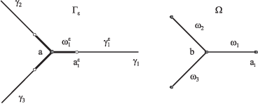
Let us consider a noncompact star graph Γ\Gamma consisting of three edges γ1\gamma_{1}, γ2\gamma_{2} and γ3\gamma_{3}. All edges are connected at the vertex aa. Then E⁡(Γ)={γ1,γ2,γ3}E(\Gamma)=\{\gamma_{1},\gamma_{2},\gamma_{3}\} and suppose that all edges are half-lines. We write ajεa_{j}^{\varepsilon} for the point of intersection of the ε\varepsilon-sphere, centered at aa, with the edge γj∈E⁡(Γ)\gamma_{j}\in E(\Gamma) and denote by Γε\Gamma_{\varepsilon} a sub-partition of Γ\Gamma containing new vertices a1εa_{1}^{\varepsilon}, a2εa_{2}^{\varepsilon} and a3εa_{3}^{\varepsilon}. Each ajεa_{j}^{\varepsilon} divides the edge γj\gamma_{j} of the graph Γ\Gamma into two edges ωjε\omega_{j}^{\varepsilon} and γjε\gamma_{j}^{\varepsilon} of the graph Γε\Gamma_{\varepsilon} (see figure 1). Let Ωε\Omega_{\varepsilon} be a star subgraph of Γε\Gamma_{\varepsilon} such that V⁡(Ωε)={a,a1ε,a2ε,a3ε}V(\Omega_{\varepsilon})=\{a,a_{1}^{\varepsilon},a_{2}^{\varepsilon},a_{3}^{\varepsilon}\} and E⁡(Ωε)={ω1ε,ω2ε,ω3ε}E(\Omega_{\varepsilon})=\{\omega_{1}^{\varepsilon},\omega_{2}^{\varepsilon},\omega_{3}^{\varepsilon}\}.

Refer to caption
Figure 1: Graphs Γε\Gamma_{\varepsilon} and Ω\Omega

By Ω⊂ℝξ3\Omega\subset\mathbb{R}^{3}_{\xi} we denote the ε−1\varepsilon^{-1}-homothety of the graph Ωε\Omega_{\varepsilon}, centered at aa. Obviously, the resulting graph does not depend on the small parameter ε\varepsilon. The graph Ω\Omega is a star with a center at the origin bb of the auxiliary space ℝξ3\mathbb{R}^{3}_{\xi} and with the vertexes aja_{j}, which are the images of the points ajεa_{j}^{\varepsilon}. The edge of Ω\Omega connecting bb to aja_{j} will be denoted by ωj\omega_{j}.

We introduce the set 𝒬={Q∈C∞​(Ω)∣∫ΩQ​𝑑Ω=0}\mathcal{Q}=\big\{Q\in C^{\infty}(\Omega)\mid\int_{\Omega}Q\,d\Omega=0\big\}. For each nonzero element Q∈𝒬Q\in\mathcal{Q} let us define the sequence

Qε​(x)={ε−2​Q​((x−a)/ε)for x∈Ωε,0for x∈Γε∖Ωε.Q_{\varepsilon}(x)=\left\{\begin{array}[]{ll}\varepsilon^{-2}Q((x-a)/\varepsilon)&\hbox{for $x\in\Omega_{\varepsilon}$,}\\ \phantom{\varepsilon^{-2}V((x-a)/}0&\hbox{for $x\in\Gamma_{\varepsilon}\setminus\Omega_{\varepsilon}$.}\end{array}\right.

The potential QεQ_{\varepsilon} is referred to as the δ′\delta^{\prime}-like potential.

In [22], it was discovered the family of Schrödinger operators on the star graph

Hε​(α,Q)​f=−f′′+(q+α​Qε)​f,\displaystyle\mathrm{H}_{\varepsilon}(\alpha,Q)f=-f^{\prime\prime}+(q+\alpha Q_{\varepsilon})f,
𝒟(Hε(α,Q))={f∈L2(Γ)∣f,f′∈AC(Γ),−f′′+(q+αQε)f∈L2(Γ),\displaystyle\mathcal{D}(\mathrm{H}_{\varepsilon}(\alpha,Q))=\Big\{f\in L_{2}(\Gamma)\mid f,\,f^{\prime}\in AC(\Gamma),\quad-f^{\prime\prime}+(q+\alpha Q_{\varepsilon})f\in L_{2}(\Gamma),
fω1ε(a)=fω2ε(a)=fω3ε(a),∑j=13d​fd​ωjε(a)=0},\displaystyle\qquad\qquad\qquad\qquad\qquad f_{\omega_{1}^{\varepsilon}}(a)=f_{\omega_{2}^{\varepsilon}}(a)=f_{\omega_{3}^{\varepsilon}}(a),\quad\sum\limits_{j=1}^{3}\frac{df}{d\omega^{\varepsilon}_{j}}(a)=0\Big\},

where Q∈𝒬Q\in\mathcal{Q}, α\alpha is a real coupling constant, and qq is a smooth real-valued potential such that qγ​(x)→+∞q_{\gamma}(x)\to+\infty as |x|→+∞\left|x\right|\to+\infty for all γ∈E⁡(Γ)\gamma\in E(\Gamma). Such behavior of qq ensures the discreteness of the spectrum of Hε​(α,Q)\mathrm{H}_{\varepsilon}(\alpha,Q). A self-adjoint operator H⁡(α,Q)\mathrm{H}(\alpha,Q) has been assigned to each pair (α,Q)(\alpha,Q). The choice of an operator is argued by the close proximity of the energy levels and the pure states for the Hamiltonians Hε​(α,Q)\mathrm{H}_{\varepsilon}(\alpha,Q) and H⁡(α,Q)\mathrm{H}(\alpha,Q) respectively. Two spectral characteristics of the function QQ are introduced in [22]: the resonant set Σ\Sigma, which is the spectrum of the eigenvalue problem

−g′′+α​Q​g=0onΩ∖V⁡(Ω),\displaystyle-g^{\prime\prime}+\alpha Qg=0\quad\hbox{on$\quad\Omega\setminus V(\Omega)$,} (2)
gω1​(b)=gω2​(b)=gω3​(b),∑j=13d​gd​ωj​(b)=0,\displaystyle\phantom{-}g_{\omega_{1}}(b)=g_{\omega_{2}}(b)=g_{\omega_{3}}(b),\quad\sum\limits_{j=1}^{3}\frac{dg}{d\omega_{j}}(b)=0, (3)
d​gd​ω1​(a1)=d​gd​ω2​(a2)=d​gd​ω3​(a3)=0,\displaystyle\phantom{-}\frac{dg}{d\omega_{1}}(a_{1})=\frac{dg}{d\omega_{2}}(a_{2})=\frac{dg}{d\omega_{3}}(a_{3})=0, (4)

and the coupling function θ:Σ→ℂ​ℙ2\theta:\,\Sigma\to\mathbb{CP}^{2}, where ℂ​ℙ2\mathbb{CP}^{2} is the complex projective plane. The spectrum of the problem (2) is real, discrete and has two accumulation points ±∞\pm\infty. It consists of simple and double eigenvalues. Write Σ1\Sigma_{1} for the subset of simple eigenvalues of the problem (2) and by Σ2\Sigma_{2} we denote the subset of double eigenvalues. The resonant set can be represented as the union of Σ1\Sigma_{1} and Σ2\Sigma_{2}.

Let α\alpha be a simple eigenvalue of the problem (2) with an eigenfunction uαu_{\alpha} such that uα2​(a1)+uα2​(a2)+uα2​(a3)=1u_{\alpha}^{2}(a_{1})+u_{\alpha}^{2}(a_{2})+u_{\alpha}^{2}(a_{3})=1, then introduce

θ1​(α)=uα​(a1),θ2​(α)=uα​(a2),θ3​(α)=uα​(a3).\theta_{1}(\alpha)=u_{\alpha}(a_{1}),\qquad\theta_{2}(\alpha)=u_{\alpha}(a_{2}),\qquad\theta_{3}(\alpha)=u_{\alpha}(a_{3}).

For α∈Σ2\alpha\in\Sigma_{2} we consider

θ1​(α)=vα​(a2)​wα​(a3)−vα​(a3)​wα​(a2),\displaystyle\theta_{1}(\alpha)=v_{\alpha}(a_{2})w_{\alpha}(a_{3})-v_{\alpha}(a_{3})w_{\alpha}(a_{2}),
θ2​(α)=vα​(a3)​wα​(a1)−vα​(a1)​wα​(a3),\displaystyle\theta_{2}(\alpha)=v_{\alpha}(a_{3})w_{\alpha}(a_{1})-v_{\alpha}(a_{1})w_{\alpha}(a_{3}),
θ3​(α)=vα​(a1)​wα​(a2)−vα​(a2)​wα​(a1),\displaystyle\theta_{3}(\alpha)=v_{\alpha}(a_{1})w_{\alpha}(a_{2})-v_{\alpha}(a_{2})w_{\alpha}(a_{1}),

where vαv_{\alpha} and wαw_{\alpha} form a base in the corresponding eigenspace such that θ12​(α)+θ22​(α)+θ32​(α)=1\theta_{1}^{2}(\alpha)+\theta_{2}^{2}(\alpha)+\theta_{3}^{2}(\alpha)=1. The coupling function is defined via θ⁡(α)=(θ1​(α),θ2​(α),θ3​(α))\theta(\alpha)=(\theta_{1}(\alpha),\theta_{2}(\alpha),\theta_{3}(\alpha)). It if easy to check that if we change a base in the eigenspace the point (θ1​(α),θ2​(α),θ3​(α))∈ℂ3(\theta_{1}(\alpha),\theta_{2}(\alpha),\theta_{3}(\alpha))\in\mathbb{C}^{3} should be replaced by (λ​θ1​(α),λ​θ2​(α),λ​θ3​(α))(\lambda\theta_{1}(\alpha),\lambda\theta_{2}(\alpha),\lambda\theta_{3}(\alpha)) with some complex λ\lambda, hence we shall find it convenient to consider θ\theta as a function from the resonant set into ℂ​ℙ2\mathbb{CP}^{2}. In the non-resonant case, when the coupling constant α\alpha does not belong to the resonant set, H⁡(α,Q)\mathrm{H}(\alpha,Q) is the direct sum of the Schrödinger operators with the potential qq on edges, subject to the Dirichlet boundary conditions at the vertex aa. If α∈Σ1\alpha\in\Sigma_{1} (the case of simple resonance), then the operator H⁡(α,Q)\mathrm{H}(\alpha,Q) acts via H⁡(α,Q)​ψ=−ψ′′+q​ψ\mathrm{H}(\alpha,Q)\psi=-\psi^{\prime\prime}+q\psi on an appropriate set of functions obeying the interface conditions

θ2​(α)​θ3​(α)​ψγ1​(a)=θ1​(α)​θ3​(α)​ψγ2​(a)=θ1​(α)​θ2​(α)​ψγ3​(a),θ1​(α)​d​ψd​γ1​(a)+θ2​(α)​d​ψd​γ2​(a)+θ3​(α)​d​ψd​γ3​(a)=0\left.\begin{array}[]{l}\theta_{2}(\alpha)\theta_{3}(\alpha)\psi_{\gamma_{1}}(a)=\theta_{1}(\alpha)\theta_{3}(\alpha)\psi_{\gamma_{2}}(a)=\theta_{1}(\alpha)\theta_{2}(\alpha)\psi_{\gamma_{3}}(a),\\ \,\qquad\theta_{1}(\alpha)\frac{d\psi}{d\gamma_{1}}(a)+\theta_{2}(\alpha)\frac{d\psi}{d\gamma_{2}}(a)+\theta_{3}(\alpha)\frac{d\psi}{d\gamma_{3}}(a)=0\end{array}\right. (5)

that can be expressed by (1) with

A=(θ3​(α)0−θ1​(α)0θ3​(α)−θ2​(α)000),B=(000000θ1​(α)θ2​(α)θ3​(α)).\mathrm{A}=\left(\begin{array}[]{ccc}\theta_{3}(\alpha)&0&-\theta_{1}(\alpha)\\ 0&\theta_{3}(\alpha)&-\theta_{2}(\alpha)\\ 0&0&0\end{array}\right),\qquad\mathrm{B}=\left(\begin{array}[]{ccc}0&0&0\\ 0&0&0\\ \theta_{1}(\alpha)&\theta_{2}(\alpha)&\theta_{3}(\alpha)\end{array}\right).

In the case of double resonance (α∈Σ2\alpha\in\Sigma_{2}), the interface conditions may be written as

θ2​(α)​θ3​(α)​d​ψd​γ1​(a)=θ1​(α)​θ3​(α)​d​ψd​γ2​(a)=θ1​(α)​θ2​(α)​d​ψd​γ3​(a),θ1​(α)​ψγ1​(a)+θ2​(α)​ψγ2​(a)+θ3​(α)​ψγ3​(a)=0\left.\begin{array}[]{l}\theta_{2}(\alpha)\theta_{3}(\alpha)\frac{d\psi}{d\gamma_{1}}(a)=\theta_{1}(\alpha)\theta_{3}(\alpha)\frac{d\psi}{d\gamma_{2}}(a)=\theta_{1}(\alpha)\theta_{2}(\alpha)\frac{d\psi}{d\gamma_{3}}(a),\\ \,\qquad\theta_{1}(\alpha)\psi_{\gamma_{1}}(a)+\theta_{2}(\alpha)\psi_{\gamma_{2}}(a)+\theta_{3}(\alpha)\psi_{\gamma_{3}}(a)=0\end{array}\right. (6)

To derive these conditions in the form (1) we need only interchange the roles of the above matrixes A\mathrm{A} and B\mathrm{B}.

If λ\lambda is an eigenvalue of the operator H⁡(α,Q)\mathrm{H}(\alpha,Q), we will denote by Pλ\mathrm{P}_{\lambda} the orthogonal projector onto the corresponding eigenspace. Let Pλ​(ε)\mathrm{P}_{\lambda}(\varepsilon) stand for the orthogonal projector onto the finite dimensional space spanned by all eigenfunctions corresponding to those eigenvalues λε\lambda_{\varepsilon} of Hε​(α,Q)\mathrm{H}_{\varepsilon}(\alpha,Q) that λε→λ\lambda_{\varepsilon}\to\lambda as ε→0\varepsilon\to 0. The results of [22] may be summed up in the following theorem.

Theorem 1.1

All eigenvalues of Hε​(α,Q)\mathrm{H}_{\varepsilon}(\alpha,Q) (except at most a finite number) are bounded as ε→0\varepsilon\to 0. Let λε\lambda_{\varepsilon} be an eigenvalue of Hε​(α,Q)\mathrm{H}_{\varepsilon}(\alpha,Q) bounded as ε→0\varepsilon\to 0, then λε\lambda_{\varepsilon} has a finite limit λ\lambda that is a point of the spectrum of H⁡(α,Q)\mathrm{H}(\alpha,Q). Moreover, ‖Pλ​(ε)−Pλ‖→0\|\mathrm{P}_{\lambda}(\varepsilon)-\mathrm{P}_{\lambda}\|\to 0 as ε→0\varepsilon\to 0. Conversely, if λ\lambda is an eigenvalue of H⁡(α,Q)\mathrm{H}(\alpha,Q), then there exists an eigenvalue λε\lambda_{\varepsilon} of Hε​(α,Q)\mathrm{H}_{\varepsilon}(\alpha,Q) such that λε→λ\lambda_{\varepsilon}\to\lambda as ε→0\varepsilon\to 0.

Although it has been showed the close proximity of the energy levels and pure states for the limiting and regularized Hamiltonians, we are still in the dark about convergence as ε→0\varepsilon\to 0 of the operators Hε​(α,Q)\mathrm{H}_{\varepsilon}(\alpha,Q) in any topology. As a result, we do not know anything about convergence of the scattering quantities or other physical characteristics. Our objective in this paper is to give one further motivation for the choice of the Hamiltonian H⁡(α,Q)\mathrm{H}(\alpha,Q). We shall study the scattering properties of the finite-range potentials α​Qε\alpha Q_{\varepsilon} on the graph Γε\Gamma_{\varepsilon} in the limit ε→0\varepsilon\to 0. We prove that the scattering coefficients depend on the intensity α\alpha and the function QQ in such a way that for all values of α\alpha the barrier α​Qε\alpha Q_{\varepsilon} is completely opaque except for the set Σ\Sigma of resonant values, at which a partial transmission through the potential occurs. It will also be shown that the scattering amplitude for the Hamiltonians Hε​(α,Q)\mathrm{H}_{\varepsilon}(\alpha,Q) and H0\mathrm{H}_{0} converges as ε→0\varepsilon\to 0 to that for the limiting Hamiltonian H⁡(α,Q)\mathrm{H}(\alpha,Q). Here the Hamiltonian H0\mathrm{H}_{0} of a free particle on Γ\Gamma acts via H0​f=−f′′\mathrm{H}_{0}f=-f^{\prime\prime} on its domain consisting of those functions from H2​(Γ)H^{2}(\Gamma) that are continuous on Γ\Gamma and satisfy the Kirchhoff boundary conditions at the vertex.

2 Scattering problem for the δ′\delta^{\prime}-like potential on the graph

Let us state the main result of this paper.

Theorem 2.1

For each k>0k>0 and α∈ℝ\alpha\in\mathbb{R} the scattering matrix for the operators Hε​(α,Q)\mathrm{H}_{\varepsilon}(\alpha,Q) and H0\mathrm{H}_{0} converge as ε→0\varepsilon\to 0 to the scattering matrix for H⁡(α,Q)\mathrm{H}(\alpha,Q) and H0\mathrm{H}_{0}.

To start with, we briefly treat stationary scattering on the graph Γ\Gamma associated with the Hamiltonians H⁡(α,Q)\mathrm{H}(\alpha,Q) and H0\mathrm{H}_{0}. From now on we assume that qq is a zero function, i.e., the operator H⁡(α,Q)\mathrm{H}(\alpha,Q) involves no potential and Hε​(α,Q)\mathrm{H}_{\varepsilon}(\alpha,Q) has only perturbed potential α​Qε\alpha Q_{\varepsilon}. It is sufficient for us to look at the nontrivial case when the coupling constant α\alpha belongs to the resonant set Σ=Σ1∪Σ2\Sigma=\Sigma_{1}\cup\Sigma_{2}, since in the opposite case the particle is always reflected. Let us introduce a natural parametrization s∈(0,+∞)s\in(0,+\infty) on each edge of Γ\Gamma and Γε\Gamma_{\varepsilon}, where s=0s=0 corresponds to the vertex aa. Consider the incoming monochromatic wave e−i​k​se^{-iks} with k>0k>0 coming from infinity along the edge γn\gamma_{n}. The corresponding wavefunction has the form

ψn​(s,k)={Tn​m​ei​k​son γm, m≠n,e−i​k​s+Tn​n​ei​k​son γn.\psi_{n}(s,k)=\left\{\begin{array}[]{ll}\phantom{e^{-iks}+}\;\;T_{nm}e^{iks}&\hbox{on $\gamma_{m}$, $\,m\neq n$,}\\ e^{-iks}+T_{nn}\,e^{iks}&\hbox{on $\gamma_{n}$.}\end{array}\right. (7)

Here Tn​nT_{nn} are the reflection coefficients, and Tn​mT_{nm} are the transmission coefficients. Substituting ψn\psi_{n} into the matching conditions (5) or (6) we derive the scattering matrix that can be expressed via the coupling function

S⁡(α)=(−1)j−1​2​(θ12​(α)−12θ1​(α)​θ2​(α)θ1​(α)​θ3​(α)θ1​(α)​θ2​(α)θ22​(α)−12θ2​(α)​θ3​(α)θ1​(α)​θ3​(α)θ2​(α)​θ3​(α)θ32​(α)−12)S(\alpha)=(-1)^{j-1}2\left(\begin{array}[]{ccc}\theta_{1}^{2}(\alpha)-\frac{1}{2}&\theta_{1}(\alpha)\theta_{2}(\alpha)&\theta_{1}(\alpha)\theta_{3}(\alpha)\\ \theta_{1}(\alpha)\theta_{2}(\alpha)&\theta_{2}^{2}(\alpha)-\frac{1}{2}&\theta_{2}(\alpha)\theta_{3}(\alpha)\\ \theta_{1}(\alpha)\theta_{3}(\alpha)&\theta_{2}(\alpha)\theta_{3}(\alpha)&\theta_{3}^{2}(\alpha)-\frac{1}{2}\end{array}\right)

if α∈Σj\alpha\in\Sigma_{j} for j=1,2j=1,2. Note that the scattering matrix does not depend on kk.

Next let us look in detail at stationary scattering for the Hamiltonians Hε​(α,Q)\mathrm{H}_{\varepsilon}(\alpha,Q) and H0\mathrm{H}_{0} and find the limit as ε→0\varepsilon\to 0 of the scattering amplitude. Consider the incoming monochromatic wave e−i​k​se^{-iks} coming from infinity along the edge γ3\gamma_{3}.

We shall seek a positive-energy solution of the problem

−y′′+α​Qε​y=k2​yon Γ∖{a},yω1​(a)=yω2​(a)=yω3​(a),∑j=13d​yd​ωj​(a)=0\displaystyle-y^{\prime\prime}+\alpha Q_{\varepsilon}y=k^{2}y\quad\hbox{on $\Gamma\setminus\{a\}$},\quad\phantom{-}y_{\omega_{1}}(a)=y_{\omega_{2}}(a)=y_{\omega_{3}}(a),\quad\sum_{j=1}^{3}\frac{dy}{d\omega_{j}}(a)=0 (8)

that coincides on Γε∖Ωε\Gamma_{\varepsilon}\setminus\Omega_{\varepsilon} with ψ3\psi_{3} given by (7). Let uα=uα​(ξ,ϰ)u_{\alpha}=u_{\alpha}(\xi,\varkappa), vα=vα​(ξ,ϰ)v_{\alpha}=v_{\alpha}(\xi,\varkappa) and wα=wα​(ξ,ϰ)w_{\alpha}=w_{\alpha}(\xi,\varkappa) be a linearly independent system of solutions of the problem

−g′′+α​Q​g=ϰ2​gon Ω∖{b},gω1​(b)=gω2​(b)=gω3​(b),∑j=13d​gd​ωj​(b)=0-g^{\prime\prime}+\alpha Qg=\varkappa^{2}g\quad\hbox{on $\Omega\setminus\{b\}$},\qquad g_{\omega_{1}}(b)=g_{\omega_{2}}(b)=g_{\omega_{3}}(b),\qquad\sum_{j=1}^{3}\frac{dg}{d\omega_{j}}(b)=0 (9)

on the graph Ω\Omega. Clearly, the functions uα​((x−a)/ε,ε​k)u_{\alpha}((x-a)/\varepsilon,\varepsilon k), vα=vα​((x−a)/ε,ε​k)v_{\alpha}=v_{\alpha}((x-a)/\varepsilon,\varepsilon k) and wα=wα​((x−a)/ε,ε​k)w_{\alpha}=w_{\alpha}((x-a)/\varepsilon,\varepsilon k) form a linearly independent system of solutions of the problem (8) on Ωε\Omega_{\varepsilon}. Hence the desired solution on Ωε\Omega_{\varepsilon} can be represented as a linear combination of this functions with the coefficients AA, BB and CC respectively. Write ϰ=ε​k\varkappa=\varepsilon k. Since the potential α​Qε\alpha Q_{\varepsilon} has discontinuities at the points a1εa_{1}^{\varepsilon}, a2εa_{2}^{\varepsilon} and a3εa_{3}^{\varepsilon}, we demand that the conditions

yγjε(ajε)=yωjε(ajε),d​yd​γjε(ajε)+d​yd​ωjε(ajε)=0,j=1,2,3\phantom{-}y_{\gamma_{j}^{\varepsilon}}(a_{j}^{\varepsilon})=y_{\omega_{j}^{\varepsilon}}(a_{j}^{\varepsilon}),\qquad\frac{dy}{d\gamma_{j}^{\varepsilon}}(a_{j}^{\varepsilon})+\frac{dy}{d\omega_{j}^{\varepsilon}}(a_{j}^{\varepsilon})=0,\quad j=1,2,3 (10)

hold. On substituting our solution into (10) we obtain the linear system M​c=r\mathrm{M}c=r for the vector of unknown coefficients c⁡(α,ϰ)=(T31,T32,T33,A,B,C)⊤c(\alpha,\varkappa)=(T_{31},T_{32},T_{33},A,B,C)^{\top}. Here r⁡(ϰ)=(0,0,0,0,e−i​ϰ,−i​ϰ​e−i​ϰ)⊤r(\varkappa)=(0,0,0,0,e^{-i\varkappa},-i\varkappa e^{-i\varkappa})^{\top} and

M⁡(α,ϰ)=(−ei​ϰ00uα​(a1,ϰ)vα​(a1,ϰ)wα​(a1,ϰ)−i​ϰ​ei​ϰ00d​uαd​ω1​(a1,ϰ)d​vαd​ω1​(a1,ϰ)d​wαd​ω1​(a1,ϰ)0−ei​ϰ0uα​(a2,ϰ)vα​(a2,ϰ)wα​(a2,ϰ)0−i​ϰ​ei​ϰ0d​uαd​ω2​(a2,ϰ)d​vαd​ω2​(a2,ϰ)d​wαd​ω2​(a2,ϰ)00−ei​ϰuα​(a3,ϰ)vα​(a3,ϰ)wα​(a3,ϰ)00−i​ϰ​ei​ϰd​uαd​ω3​(a3,ϰ)d​vαd​ω3​(a3,ϰ)d​wαd​ω3​(a3,ϰ)).\qquad\mathrm{M}(\alpha,\varkappa)=\left(\begin{array}[]{cccccc}-e^{i\varkappa}&0&0&u_{\alpha}(a_{1},\varkappa)&v_{\alpha}(a_{1},\varkappa)&w_{\alpha}(a_{1},\varkappa)\\ -i\varkappa e^{i\varkappa}&0&0&\frac{du_{\alpha}}{d\omega_{1}}(a_{1},\varkappa)&\frac{dv_{\alpha}}{d\omega_{1}}(a_{1},\varkappa)&\frac{dw_{\alpha}}{d\omega_{1}}(a_{1},\varkappa)\\ 0&-e^{i\varkappa}&0&u_{\alpha}(a_{2},\varkappa)&v_{\alpha}(a_{2},\varkappa)&w_{\alpha}(a_{2},\varkappa)\\ 0&-i\varkappa e^{i\varkappa}&0&\frac{du_{\alpha}}{d\omega_{2}}(a_{2},\varkappa)&\frac{dv_{\alpha}}{d\omega_{2}}(a_{2},\varkappa)&\frac{dw_{\alpha}}{d\omega_{2}}(a_{2},\varkappa)\\ 0&0&-e^{i\varkappa}&u_{\alpha}(a_{3},\varkappa)&v_{\alpha}(a_{3},\varkappa)&w_{\alpha}(a_{3},\varkappa)\\ 0&0&-i\varkappa e^{i\varkappa}&\frac{du_{\alpha}}{d\omega_{3}}(a_{3},\varkappa)&\frac{dv_{\alpha}}{d\omega_{3}}(a_{3},\varkappa)&\frac{dw_{\alpha}}{d\omega_{3}}(a_{3},\varkappa)\end{array}\right).

Clearly, the functions uα​(⋅,0)u_{\alpha}(\cdot,0), vα​(⋅,0)v_{\alpha}(\cdot,0) and wα​(⋅,0)w_{\alpha}(\cdot,0) form a linearly independent system of solutions of the problem (2), (3). In what follows we shall omit the second argument of these functions and keep in mind that it equals zero. We introduce the determinants

h0​(α)=|uα​(a1)vα​(a1)wα​(a1)uα​(a2)vα​(a2)wα​(a2)uα​(a3)vα​(a3)wα​(a3)|,h1​(α)=|d​uαd​ω1​(a1)d​vαd​ω1​(a1)d​wαd​ω1​(a1)d​uαd​ω2​(a2)d​vαd​ω2​(a2)d​wαd​ω2​(a2)d​uαd​ω3​(a3)d​vαd​ω3​(a3)d​wαd​ω3​(a3)|.h_{0}(\alpha)=\left|\begin{array}[]{ccc}u_{\alpha}(a_{1})&v_{\alpha}(a_{1})&w_{\alpha}(a_{1})\\ u_{\alpha}(a_{2})&v_{\alpha}(a_{2})&w_{\alpha}(a_{2})\\ u_{\alpha}(a_{3})&v_{\alpha}(a_{3})&w_{\alpha}(a_{3})\end{array}\right|,\qquad h_{1}(\alpha)=\left|\begin{array}[]{ccc}\frac{du_{\alpha}}{d\omega_{1}}(a_{1})&\frac{dv_{\alpha}}{d\omega_{1}}(a_{1})&\frac{dw_{\alpha}}{d\omega_{1}}(a_{1})\\ \frac{du_{\alpha}}{d\omega_{2}}(a_{2})&\frac{dv_{\alpha}}{d\omega_{2}}(a_{2})&\frac{dw_{\alpha}}{d\omega_{2}}(a_{2})\\ \frac{du_{\alpha}}{d\omega_{3}}(a_{3})&\frac{dv_{\alpha}}{d\omega_{3}}(a_{3})&\frac{dw_{\alpha}}{d\omega_{3}}(a_{3})\end{array}\right|.

Let us also consider the function hn​mh_{nm}, which is just the determinant h1−nh_{1-n} with the mt​hm^{th}-row replaced by the mt​hm^{th}-row of hnh_{n} for n=0,1n=0,1; m=1,2,3m=1,2,3.

Let us denote by Δ⁡(ϰ,α)\Delta(\varkappa,\alpha) the determinant of the matrix M⁡(ϰ,α)\mathrm{M}(\varkappa,\alpha). It admits the asymptotic expansion

Δ(ϰ,α)=h1(α)+iϰ{3h1(α)−H0(α)}+ϰ2{−9/2h1(α)+3H0(α)−H1(α)}+O(ϰ3)\displaystyle\Delta(\varkappa,\alpha)=h_{1}(\alpha)+i\varkappa\{3h_{1}(\alpha)-H_{0}(\alpha)\}+\varkappa^{2}\{-9/2\,h_{1}(\alpha)+3H_{0}(\alpha)-H_{1}(\alpha)\}+O(\varkappa^{3})

as ϰ→0\varkappa\to 0, where Hn​(α)=∑m=13hn​m​(α)H_{n}(\alpha)=\sum_{m=1}^{3}h_{nm}(\alpha) for n=0,1n=0,1. Employing Cramer’s rule, we derive

T31​(ϰ,α)=−2​i​ϰ​(1+i​ϰ)Δ⁡(ϰ,α)|uα​(a1)vα​(a1)wα​(a1)d​uαd​ω1​(a1)d​vαd​ω1​(a1)d​wαd​ω1​(a1)d​uαd​ω2​(a2)d​vαd​ω2​(a2)d​wαd​ω2​(a2)|−2​ϰ2Δ⁡(ϰ,α)​|uα​(a1)vα​(a1)wα​(a1)d​uαd​ω1​(a1)d​vαd​ω1​(a1)d​wαd​ω1​(a1)uα​(a2)vα​(a2)wα​(a2)|+O⁡(ϰ3),\displaystyle\left.\begin{array}[]{ll}T_{31}(\varkappa,\alpha)=\frac{-2i\varkappa(1+i\varkappa)}{\Delta(\varkappa,\alpha)}&\left|\begin{array}[]{ccc}u_{\alpha}(a_{1})&v_{\alpha}(a_{1})&w_{\alpha}(a_{1})\\ \frac{du_{\alpha}}{d\omega_{1}}(a_{1})&\frac{dv_{\alpha}}{d\omega_{1}}(a_{1})&\frac{dw_{\alpha}}{d\omega_{1}}(a_{1})\\ \frac{du_{\alpha}}{d\omega_{2}}(a_{2})&\frac{dv_{\alpha}}{d\omega_{2}}(a_{2})&\frac{dw_{\alpha}}{d\omega_{2}}(a_{2})\end{array}\right|\\ &\qquad\qquad-\frac{2\varkappa^{2}}{\Delta(\varkappa,\alpha)}\left|\begin{array}[]{ccc}u_{\alpha}(a_{1})&v_{\alpha}(a_{1})&w_{\alpha}(a_{1})\\ \frac{du_{\alpha}}{d\omega_{1}}(a_{1})&\frac{dv_{\alpha}}{d\omega_{1}}(a_{1})&\frac{dw_{\alpha}}{d\omega_{1}}(a_{1})\\ u_{\alpha}(a_{2})&v_{\alpha}(a_{2})&w_{\alpha}(a_{2})\end{array}\right|+O(\varkappa^{3}),\end{array}\right.
T32​(ϰ,α)=2​i​ϰ​(1+i​ϰ)Δ⁡(ϰ,α)|d​uαd​ω1​(a1)d​vαd​ω1​(a1)d​wαd​ω1​(a1)uα​(a2)vα​(a2)wα​(a2)d​uαd​ω2​(a2)d​vαd​ω2​(a2)d​wαd​ω2​(a2)|+2​ϰ2Δ⁡(ϰ,α)​|uα​(a1)vα​(a1)wα​(a1)uα​(a2)vα​(a2)wα​(a2)d​uαd​ω2​(a2)d​vαd​ω2​(a2)d​wαd​ω2​(a2)|+O⁡(ϰ3),\displaystyle\left.\begin{array}[]{ll}T_{32}(\varkappa,\alpha)=\frac{2i\varkappa(1+i\varkappa)}{\Delta(\varkappa,\alpha)}&\left|\begin{array}[]{ccc}\frac{du_{\alpha}}{d\omega_{1}}(a_{1})&\frac{dv_{\alpha}}{d\omega_{1}}(a_{1})&\frac{dw_{\alpha}}{d\omega_{1}}(a_{1})\\ u_{\alpha}(a_{2})&v_{\alpha}(a_{2})&w_{\alpha}(a_{2})\\ \frac{du_{\alpha}}{d\omega_{2}}(a_{2})&\frac{dv_{\alpha}}{d\omega_{2}}(a_{2})&\frac{dw_{\alpha}}{d\omega_{2}}(a_{2})\end{array}\right|\\ &\qquad\qquad+\frac{2\varkappa^{2}}{\Delta(\varkappa,\alpha)}\left|\begin{array}[]{ccc}u_{\alpha}(a_{1})&v_{\alpha}(a_{1})&w_{\alpha}(a_{1})\\ u_{\alpha}(a_{2})&v_{\alpha}(a_{2})&w_{\alpha}(a_{2})\\ \frac{du_{\alpha}}{d\omega_{2}}(a_{2})&\frac{dv_{\alpha}}{d\omega_{2}}(a_{2})&\frac{dw_{\alpha}}{d\omega_{2}}(a_{2})\end{array}\right|+O(\varkappa^{3}),\end{array}\right.
T33​(ϰ,α)=(Δ(ϰ,α))−1[−h1(α)+iϰ{H0(α)−2h03(α)−h1(α)}−ϰ2{H1(α)+H0(α)−2(h13(α)+h03(α))−1/2h1(α)}]+O(ϰ3)\displaystyle\left.\begin{array}[]{ll}T_{33}(\varkappa,\alpha)=&\big(\Delta(\varkappa,\alpha)\big)^{-1}\Big[-h_{1}(\alpha)+i\varkappa\big\{H_{0}(\alpha)-2h_{03}(\alpha)-h_{1}(\alpha)\big\}\\ &-\varkappa^{2}\big\{H_{1}(\alpha)+H_{0}(\alpha)-2(h_{13}(\alpha)+h_{03}(\alpha))-1/2h_{1}(\alpha)\big\}\Big]+O(\varkappa^{3})\end{array}\right.

as ϰ→0\varkappa\to 0. Similar asymptotics can be derived without difficulty in the case, when the wave package comes from infinity along γ1\gamma_{1} or γ2\gamma_{2}. We shall study the asymptotic behavior as ϰ→0\varkappa\to 0 of the scattering coefficients. Three cases are to be distinguished: Δ⁡(ϰ,α)=O⁡(1)\Delta(\varkappa,\alpha)=O(1), Δ⁡(ϰ,α)=O⁡(ϰ)\Delta(\varkappa,\alpha)=O(\varkappa) and Δ⁡(ϰ,α)=O⁡(ϰ2)\Delta(\varkappa,\alpha)=O(\varkappa^{2}) as ϰ→0\varkappa\to 0.

Lemma 2.2

The set of roots of the equation h1​(z)=0h_{1}(z)=0 coincides with the resonant set, i.e., h1h_{1} is a characteristic determinant of the eigenvalue problem (2)–(4).

Proof. It is easily seen that the system uαu_{\alpha}, vαv_{\alpha} and wαw_{\alpha} of solutions of the problem (9) may be chosen so that

uα​(b)=0,d​uαd​ω1​(b)=0,d​uαd​ω2​(b)=1,\displaystyle u_{\alpha}(b)=0,\qquad\frac{du_{\alpha}}{d\omega_{1}}(b)=0,\qquad\frac{du_{\alpha}}{d\omega_{2}}(b)=1,
vα​(b)=0,d​vαd​ω2​(b)=0,d​vαd​ω1​(b)=1.\displaystyle v_{\alpha}(b)=0,\qquad\frac{dv_{\alpha}}{d\omega_{2}}(b)=0,\qquad\frac{dv_{\alpha}}{d\omega_{1}}(b)=1.

Clearly, uαu_{\alpha} vanishes on ω1\omega_{1}, and vαv_{\alpha} vanishes on ω2\omega_{2}. Let us consider the linear combination

g=d​vαd​ω1​(a1)​d​wαd​ω2​(a2)​uα+d​uαd​ω2​(a2)​d​wαd​ω1​(a1)​vα−d​uαd​ω2​(a2)​d​vαd​ω1​(a1)​wα.g=\frac{dv_{\alpha}}{d\omega_{1}}(a_{1})\frac{dw_{\alpha}}{d\omega_{2}}(a_{2})u_{\alpha}+\frac{du_{\alpha}}{d\omega_{2}}(a_{2})\frac{dw_{\alpha}}{d\omega_{1}}(a_{1})v_{\alpha}-\frac{du_{\alpha}}{d\omega_{2}}(a_{2})\frac{dv_{\alpha}}{d\omega_{1}}(a_{1})w_{\alpha}. (32)

By construction d​gd​ω1​(a1)=d​gd​ω2​(a2)=0\frac{dg}{d\omega_{1}}(a_{1})=\frac{dg}{d\omega_{2}}(a_{2})=0 and d​gd​ω3​(a3)=h1​(α)\frac{dg}{d\omega_{3}}(a_{3})=h_{1}(\alpha). Hence if h1​(α)=0h_{1}(\alpha)=0 and gg is nontrivial on Ω\Omega, then gg is an eigenfunction of the problem (2), corresponding to α\alpha, and therefore α∈Σ\alpha\in\Sigma.

Note that at least one of the values d​uαd​ωj​(aj)\frac{du_{\alpha}}{d\omega_{j}}(a_{j}), d​vαd​ωj​(aj)\frac{dv_{\alpha}}{d\omega_{j}}(a_{j}) or d​wαd​ωj​(aj)\frac{dw_{\alpha}}{d\omega_{j}}(a_{j}) is different from zero for j=1,2,3j=1,2,3. Now consider the exceptional case, when gg is trivial, i.e., all coefficients in (32) equal zero. We show then that both values d​uαd​ω2​(a2)\frac{du_{\alpha}}{d\omega_{2}}(a_{2}) and d​vαd​ω1​(a1)\frac{dv_{\alpha}}{d\omega_{1}}(a_{1}) are zero. Conversely, suppose that d​vαd​ω1​(a1)≠0\frac{dv_{\alpha}}{d\omega_{1}}(a_{1})\neq 0. Since d​vαd​ω1​(a1)​d​wαd​ω2​(a2)=0\frac{dv_{\alpha}}{d\omega_{1}}(a_{1})\frac{dw_{\alpha}}{d\omega_{2}}(a_{2})=0, one obtains d​uαd​ω2​(a2)=d​vαd​ω2​(a2)=d​wαd​ω2​(a2)=0\frac{du_{\alpha}}{d\omega_{2}}(a_{2})=\frac{dv_{\alpha}}{d\omega_{2}}(a_{2})=\frac{dw_{\alpha}}{d\omega_{2}}(a_{2})=0, a contradiction. Similarly, d​uαd​ω2​(a2)=0\frac{du_{\alpha}}{d\omega_{2}}(a_{2})=0. It follows that d​uαd​ω1​(a1)=d​uαd​ω2​(a2)=0\frac{du_{\alpha}}{d\omega_{1}}(a_{1})=\frac{du_{\alpha}}{d\omega_{2}}(a_{2})=0 and d​vαd​ω1​(a1)=d​vαd​ω2​(a2)=0\frac{dv_{\alpha}}{d\omega_{1}}(a_{1})=\frac{dv_{\alpha}}{d\omega_{2}}(a_{2})=0. Thus the function g1=d​vαd​ω3​(a3)​uα−d​uαd​ω3​(a3)​vαg_{1}=\frac{dv_{\alpha}}{d\omega_{3}}(a_{3})u_{\alpha}-\frac{du_{\alpha}}{d\omega_{3}}(a_{3})v_{\alpha} satisfies d​g1d​ω1​(a1)=d​g1d​ω2​(a2)=d​g1d​ω3​(a3)=0\frac{dg_{1}}{d\omega_{1}}(a_{1})=\frac{dg_{1}}{d\omega_{2}}(a_{2})=\frac{dg_{1}}{d\omega_{3}}(a_{3})=0. If g1g_{1} is nontrivial on Ω\Omega, then it is an eigenfunction of the problem (2), corresponding to α\alpha. If not, then uαu_{\alpha} would be a desired eigenfunction.

What is left is to show that α∈Σ\alpha\in\Sigma implies h1​(α)=0h_{1}(\alpha)=0. If we choose the new base uαu_{\alpha}, vαv_{\alpha} and wαw_{\alpha} such that uαu_{\alpha} is an eigenfunction of the problem (2)–(4) corresponding to α\alpha, then the first column of the determinant is zero and the assertion follows. □\square

Lemma 2.3

The set of roots of the equation H0​(z)=0H_{0}(z)=0 that belongs to the resonant set coincides with Σ2\Sigma_{2}.

Proof. Suppose, contrary to our claim, that there exists α∈Σ1\alpha\in\Sigma_{1} such that H0​(α)=0H_{0}(\alpha)=0. We choose the new linearly independent system uαu_{\alpha}, vαv_{\alpha} and wαw_{\alpha} such that uαu_{\alpha} is an eigenfunction of the problem (2)–(4) corresponding to α\alpha. Write V=(d​vαd​ω1​(a1),d​vαd​ω2​(a2),d​vαd​ω3​(a3))V=(\frac{dv_{\alpha}}{d\omega_{1}}(a_{1}),\frac{dv_{\alpha}}{d\omega_{2}}(a_{2}),\frac{dv_{\alpha}}{d\omega_{3}}(a_{3})) and W=(d​wαd​ω1​(a1),d​wαd​ω2​(a2),d​wαd​ω3​(a3))W=(\frac{dw_{\alpha}}{d\omega_{1}}(a_{1}),\frac{dw_{\alpha}}{d\omega_{2}}(a_{2}),\frac{dw_{\alpha}}{d\omega_{3}}(a_{3})). These vectors are linearly independent. Indeed, in the opposite case there exists a nonzero number λ\lambda such that V=λ​WV=\lambda W. Therefore vα−λ​wαv_{\alpha}-\lambda w_{\alpha} is an eigenfunction of the problem (2)–(4) corresponding to α\alpha that is linearly independent with uαu_{\alpha}, a contradiction.

In view of the Lagrange identities

uα​(a1)​d​vαd​ω1​(a1)+uα​(a2)​d​vαd​ω2​(a2)+uα​(a3)​d​vαd​ω3​(a3)=0,\displaystyle u_{\alpha}(a_{1})\frac{dv_{\alpha}}{d\omega_{1}}(a_{1})+u_{\alpha}(a_{2})\frac{dv_{\alpha}}{d\omega_{2}}(a_{2})+u_{\alpha}(a_{3})\frac{dv_{\alpha}}{d\omega_{3}}(a_{3})=0,
uα​(a1)​d​wαd​ω1​(a1)+uα​(a2)​d​wαd​ω2​(a2)+uα​(a3)​d​wαd​ω3​(a3)=0\displaystyle u_{\alpha}(a_{1})\frac{dw_{\alpha}}{d\omega_{1}}(a_{1})+u_{\alpha}(a_{2})\frac{dw_{\alpha}}{d\omega_{2}}(a_{2})+u_{\alpha}(a_{3})\frac{dw_{\alpha}}{d\omega_{3}}(a_{3})=0

the vector U=(uα​(a1),uα​(a2),uα​(a3))U=(u_{\alpha}(a_{1}),u_{\alpha}(a_{2}),u_{\alpha}(a_{3})) is orthogonal to both vectors VV and WW. The identity H0​(α)=0H_{0}(\alpha)=0 can be written as

uα​(a1)​|d​vαd​ω2​(a2)d​vαd​ω3​(a3)d​wαd​ω2​(a2)d​wαd​ω3​(a3)|+uα​(a2)​|d​vαd​ω3​(a3)d​vαd​ω1​(a1)d​wαd​ω3​(a3)d​wαd​ω1​(a1)|+uα​(a3)​|d​vαd​ω1​(a1)d​vαd​ω2​(a2)d​wαd​ω1​(a1)d​wαd​ω2​(a2)|=0.\displaystyle\left.\begin{array}[]{l}u_{\alpha}(a_{1})\left|\begin{array}[]{cc}\frac{dv_{\alpha}}{d\omega_{2}}(a_{2})&\frac{dv_{\alpha}}{d\omega_{3}}(a_{3})\\ \frac{dw_{\alpha}}{d\omega_{2}}(a_{2})&\frac{dw_{\alpha}}{d\omega_{3}}(a_{3})\end{array}\right|+u_{\alpha}(a_{2})\left|\begin{array}[]{cc}\frac{dv_{\alpha}}{d\omega_{3}}(a_{3})&\frac{dv_{\alpha}}{d\omega_{1}}(a_{1})\\ \frac{dw_{\alpha}}{d\omega_{3}}(a_{3})&\frac{dw_{\alpha}}{d\omega_{1}}(a_{1})\end{array}\right|\\ \qquad\qquad\qquad\qquad\qquad\qquad\qquad\qquad\qquad+u_{\alpha}(a_{3})\left|\begin{array}[]{cc}\frac{dv_{\alpha}}{d\omega_{1}}(a_{1})&\frac{dv_{\alpha}}{d\omega_{2}}(a_{2})\\ \frac{dw_{\alpha}}{d\omega_{1}}(a_{1})&\frac{dw_{\alpha}}{d\omega_{2}}(a_{2})\end{array}\right|=0.\end{array}\right.

It follows that UU is orthogonal to the vector product V×WV\times W, hence that UU is a zero vector, i.e., uα​(a1)=uα​(a2)=uα​(a3)=0u_{\alpha}(a_{1})=u_{\alpha}(a_{2})=u_{\alpha}(a_{3})=0, and finally that uαu_{\alpha} is a zero function, which is impossible.

Let α\alpha belong to Σ2\Sigma_{2}. We select a linearly independent system uαu_{\alpha}, vαv_{\alpha} and wαw_{\alpha} such that uαu_{\alpha} and vαv_{\alpha} form a base in the corresponding eigenspace. Obviously, the determinant H0​(α)H_{0}(\alpha) vanishes, and the proof is complete. □\square

Remark 2.4

The roots of the equation h1​(z)=0h_{1}(z)=0 as well as H0​(z)=0H_{0}(z)=0 do not depend on the choice of the linearly independent system of solutions of the problem (9).

Lemma 2.5

The function H1H_{1} is different from zero on Σ2\Sigma_{2}.

Proof. On the contrary, suppose that there exists α∈Σ2\alpha\in\Sigma_{2} such that H1​(α)=0H_{1}(\alpha)=0. Let us select the system uαu_{\alpha}, vαv_{\alpha} and wαw_{\alpha} of linearly independent solutions of the problem (9) such that uαu_{\alpha} and vαv_{\alpha} are eigenfunctions of the problem (2)–(4) corresponding to α\alpha. Set U=(uα​(a1),uα​(a2),uα​(a3))U=(u_{\alpha}(a_{1}),u_{\alpha}(a_{2}),u_{\alpha}(a_{3})) and V=(vα​(a1),vα​(a2),vα​(a3))V=(v_{\alpha}(a_{1}),v_{\alpha}(a_{2}),v_{\alpha}(a_{3})). Note that the vectors UU and VV are linearly independent, since in the opposite case the functions uαu_{\alpha} and vαv_{\alpha} would be linearly dependent.

From the Lagrange identities

uα​(a1)​d​wαd​ω1​(a1)+uα​(a2)​d​wαd​ω2​(a2)+uα​(a3)​d​wαd​ω3​(a3)=0\displaystyle u_{\alpha}(a_{1})\frac{dw_{\alpha}}{d\omega_{1}}(a_{1})+u_{\alpha}(a_{2})\frac{dw_{\alpha}}{d\omega_{2}}(a_{2})+u_{\alpha}(a_{3})\frac{dw_{\alpha}}{d\omega_{3}}(a_{3})=0
vα​(a1)​d​wαd​ω1​(a1)+vα​(a2)​d​wαd​ω2​(a2)+vα​(a3)​d​wαd​ω3​(a3)=0\displaystyle v_{\alpha}(a_{1})\frac{dw_{\alpha}}{d\omega_{1}}(a_{1})+v_{\alpha}(a_{2})\frac{dw_{\alpha}}{d\omega_{2}}(a_{2})+v_{\alpha}(a_{3})\frac{dw_{\alpha}}{d\omega_{3}}(a_{3})=0

it follows that the vector W=(d​wαd​ω1​(a1),d​wαd​ω2​(a2),d​wαd​ω3​(a3))W=(\frac{dw_{\alpha}}{d\omega_{1}}(a_{1}),\frac{dw_{\alpha}}{d\omega_{2}}(a_{2}),\frac{dw_{\alpha}}{d\omega_{3}}(a_{3})) is orthogonal to UU and VV. The identity H1​(α)=0H_{1}(\alpha)=0 can be written in the form

d​wαd​ω1​(a1)​|uα​(a2)uα​(a3)vα​(a2)vα​(a3)|+d​wαd​ω2​(a2)​|uα​(a3)uα​(a1)vα​(a3)vα​(a1)|\displaystyle\frac{dw_{\alpha}}{d\omega_{1}}(a_{1})\left|\begin{array}[]{cc}u_{\alpha}(a_{2})&u_{\alpha}(a_{3})\\ v_{\alpha}(a_{2})&v_{\alpha}(a_{3})\end{array}\right|+\frac{dw_{\alpha}}{d\omega_{2}}(a_{2})\left|\begin{array}[]{cc}u_{\alpha}(a_{3})&u_{\alpha}(a_{1})\\ v_{\alpha}(a_{3})&v_{\alpha}(a_{1})\end{array}\right|
+d​wαd​ω3​(a3)​|uα​(a1)uα​(a2)vα​(a1)vα​(a2)|=0.\displaystyle\qquad\qquad\qquad\qquad\qquad\qquad\qquad+\frac{dw_{\alpha}}{d\omega_{3}}(a_{3})\left|\begin{array}[]{cc}u_{\alpha}(a_{1})&u_{\alpha}(a_{2})\\ v_{\alpha}(a_{1})&v_{\alpha}(a_{2})\end{array}\right|=0.

Consequently, WW is orthogonal to the vector product U×VU\times V. Analysis similar to that in the proof of the previous lemma gives the assertion of the lemma. □\square

We are now in a position to prove the main result. Without loss of generality we establish the convergence of the transmission coefficient T31​(ε​k,α)T_{31}(\varepsilon k,\alpha) as ε→0\varepsilon\to 0. Other coefficients may be handled in much the same way.

Proof of Theorem 2.1. The non-resonant case. Since α\alpha is not a resonant coupling constant, h1​(α)≠0h_{1}(\alpha)\neq 0. From (2) it immediately follows that T31​(ε​k,α)=O⁡(ε​k)T_{31}(\varepsilon k,\alpha)=O(\varepsilon k) as ε→0\varepsilon\to 0.

The case of simple resonance. If α∈Σ1\alpha\in\Sigma_{1}, then h1​(α)=0h_{1}(\alpha)=0 and H0​(α)≠0H_{0}(\alpha)\neq 0 in light of Lemmas 2.2, 2.3. By (2)

T31​(ε​k,α)=2H0​(α)​|uα​(a1)vα​(a1)wα​(a1)d​uαd​ω1​(a1)d​vαd​ω1​(a1)d​wαd​ω1​(a1)d​uαd​ω2​(a2)d​vαd​ω2​(a2)d​wαd​ω2​(a2)|+O⁡(ε​k),ε→0.T_{31}(\varepsilon k,\alpha)=\frac{2}{H_{0}(\alpha)}\left|\begin{array}[]{ccc}u_{\alpha}(a_{1})&v_{\alpha}(a_{1})&w_{\alpha}(a_{1})\\ \frac{du_{\alpha}}{d\omega_{1}}(a_{1})&\frac{dv_{\alpha}}{d\omega_{1}}(a_{1})&\frac{dw_{\alpha}}{d\omega_{1}}(a_{1})\\ \frac{du_{\alpha}}{d\omega_{2}}(a_{2})&\frac{dv_{\alpha}}{d\omega_{2}}(a_{2})&\frac{dw_{\alpha}}{d\omega_{2}}(a_{2})\end{array}\right|+O(\varepsilon k),\qquad\varepsilon\to 0.

We continue by choosing the new linearly independent system uαu_{\alpha}, vαv_{\alpha} and wαw_{\alpha} such that uαu_{\alpha} is an eigenfunction of the problem (2)–(4) corresponding to α\alpha satisfying the condition uα2​(a1)+uα2​(a2)+uα2​(a3)=1u_{\alpha}^{2}(a_{1})+u_{\alpha}^{2}(a_{2})+u_{\alpha}^{2}(a_{3})=1 and d​vαd​ω2​(a2)=0\frac{dv_{\alpha}}{d\omega_{2}}(a_{2})=0. Observe that

T31​(0,α)=2​θ1​(α)​d​vαd​ω1​(a1)​d​wαd​ω2​(a2)​H0−1​(α).T_{31}(0,\alpha)=2\theta_{1}(\alpha)\frac{dv_{\alpha}}{d\omega_{1}}(a_{1})\frac{dw_{\alpha}}{d\omega_{2}}(a_{2})H^{-1}_{0}(\alpha). (38)

Now let us express T31​(0,α)T_{31}(0,\alpha) via the coupling function. Taking into account the Lagrange identities we see that

uα​(a1)uα​(a3)=−d​vαd​ω3​(a3)d​vαd​ω1​(a1),uα​(a2)uα​(a3)=d​vαd​ω3​(a3)​d​wαd​ω1​(a1)−d​vαd​ω1​(a1)​d​wαd​ω3​(a3)d​vαd​ω1​(a1)​d​wαd​ω2​(a2).\frac{u_{\alpha}(a_{1})}{u_{\alpha}(a_{3})}=-\frac{\frac{dv_{\alpha}}{d\omega_{3}}(a_{3})}{\frac{dv_{\alpha}}{d\omega_{1}}(a_{1})},\qquad\frac{u_{\alpha}(a_{2})}{u_{\alpha}(a_{3})}=\frac{\frac{dv_{\alpha}}{d\omega_{3}}(a_{3})\frac{dw_{\alpha}}{d\omega_{1}}(a_{1})-\frac{dv_{\alpha}}{d\omega_{1}}(a_{1})\frac{dw_{\alpha}}{d\omega_{3}}(a_{3})}{\frac{dv_{\alpha}}{d\omega_{1}}(a_{1})\frac{dw_{\alpha}}{d\omega_{2}}(a_{2})}.

Therefore

h01​(α)=−uα​(a1)​d​vαd​ω3​(a3)​d​wαd​ω2​(a2)=uα2​(a1)​d​vαd​ω1​(a1)​d​wαd​ω2​(a2)θ3​(α),\displaystyle h_{01}(\alpha)=-u_{\alpha}(a_{1})\frac{dv_{\alpha}}{d\omega_{3}}(a_{3})\frac{dw_{\alpha}}{d\omega_{2}}(a_{2})=\frac{u^{2}_{\alpha}(a_{1})\frac{dv_{\alpha}}{d\omega_{1}}(a_{1})\frac{dw_{\alpha}}{d\omega_{2}}(a_{2})}{\theta_{3}(\alpha)}, (39)
h02​(α)=uα​(a2)​{d​vαd​ω3​(a3)​d​wαd​ω1​(a1)−d​vαd​ω1​(a1)​d​wαd​ω3​(a3)}=uα2​(a2)​d​vαd​ω1​(a1)​d​wαd​ω2​(a2)θ3​(α).\displaystyle h_{02}(\alpha)=u_{\alpha}(a_{2})\Big\{\frac{dv_{\alpha}}{d\omega_{3}}(a_{3})\frac{dw_{\alpha}}{d\omega_{1}}(a_{1})-\frac{dv_{\alpha}}{d\omega_{1}}(a_{1})\frac{dw_{\alpha}}{d\omega_{3}}(a_{3})\Big\}=\frac{u^{2}_{\alpha}(a_{2})\frac{dv_{\alpha}}{d\omega_{1}}(a_{1})\frac{dw_{\alpha}}{d\omega_{2}}(a_{2})}{\theta_{3}(\alpha)}. (40)

By construction h03​(α)=uα2​(a3)​d​vαd​ω1​(a1)​d​wαd​ω2​(a2)/θ3​(α)h_{03}(\alpha)=u^{2}_{\alpha}(a_{3})\frac{dv_{\alpha}}{d\omega_{1}}(a_{1})\frac{dw_{\alpha}}{d\omega_{2}}(a_{2})/\theta_{3}(\alpha). Recall that H0​(α)=h01​(α)+h02​(α)+h03​(α)H_{0}(\alpha)=h_{01}(\alpha)+h_{02}(\alpha)+h_{03}(\alpha). Combining (39) and (40) yields

H0=d​vαd​ω1​(a1)​d​wαd​ω2​(a2)θ3​(α)​{uα2​(a1)+uα2​(a2)+uα2​(a3)}=d​vαd​ω1​(a1)​d​wαd​ω2​(a2)θ3​(α).H_{0}=\frac{\frac{dv_{\alpha}}{d\omega_{1}}(a_{1})\frac{dw_{\alpha}}{d\omega_{2}}(a_{2})}{\theta_{3}(\alpha)}\{u^{2}_{\alpha}(a_{1})+u^{2}_{\alpha}(a_{2})+u^{2}_{\alpha}(a_{3})\}=\frac{\frac{dv_{\alpha}}{d\omega_{1}}(a_{1})\frac{dw_{\alpha}}{d\omega_{2}}(a_{2})}{\theta_{3}(\alpha)}.

Then by (38)

T31​(0,α)=2​θ1​(α)​θ3​(α)=T31​(α).T_{31}(0,\alpha)=2\theta_{1}(\alpha)\theta_{3}(\alpha)=T_{31}(\alpha).

The case of double resonance. Finally suppose that α∈Σ2\alpha\in\Sigma_{2}. By Lemmas 2.2, 2.3 and 2.5 we have h1​(α)=H0​(α)=0h_{1}(\alpha)=H_{0}(\alpha)=0 and H1​(α)≠0H_{1}(\alpha)\neq 0, thus

T31​(ε​k,α)=2H1​(α)​|uα​(a1)vα​(a1)wα​(a1)d​uαd​ω1​(a1)d​vαd​ω1​(a1)d​wαd​ω1​(a1)uα​(a2)vα​(a2)wα​(a2)|+O⁡(ε​k),ε→0T_{31}(\varepsilon k,\alpha)=\frac{2}{H_{1}(\alpha)}\left|\begin{array}[]{ccc}u_{\alpha}(a_{1})&v_{\alpha}(a_{1})&w_{\alpha}(a_{1})\\ \frac{du_{\alpha}}{d\omega_{1}}(a_{1})&\frac{dv_{\alpha}}{d\omega_{1}}(a_{1})&\frac{dw_{\alpha}}{d\omega_{1}}(a_{1})\\ u_{\alpha}(a_{2})&v_{\alpha}(a_{2})&w_{\alpha}(a_{2})\end{array}\right|+O(\varepsilon k),\qquad\varepsilon\to 0

by (2). Let us choose the new base uαu_{\alpha}, vαv_{\alpha} and wαw_{\alpha} such that uαu_{\alpha} and vαv_{\alpha} are eigenfunctions of the problem (2) corresponding to α\alpha satisfying θ12​(α)+θ22​(α)+θ32​(α)=1\theta_{1}^{2}(\alpha)+\theta_{2}^{2}(\alpha)+\theta_{3}^{2}(\alpha)=1. Consequently,

T31​(0,α)=−2​θ3​(α)​d​wαd​ω1​(a1)​H1−1​(α).T_{31}(0,\alpha)=-2\theta_{3}(\alpha)\frac{dw_{\alpha}}{d\omega_{1}}(a_{1})H_{1}^{-1}(\alpha).

Since the Lagrange identities hold it follows that

d​wαd​ω1​(a1)θ1​(α)=d​wαd​ω2​(a2)θ2​(α)=d​wαd​ω3​(a3)θ3​(α).\frac{\frac{dw_{\alpha}}{d\omega_{1}}(a_{1})}{\theta_{1}(\alpha)}=\frac{\frac{dw_{\alpha}}{d\omega_{2}}(a_{2})}{\theta_{2}(\alpha)}=\frac{\frac{dw_{\alpha}}{d\omega_{3}}(a_{3})}{\theta_{3}(\alpha)}.

We thus get

h11​(α)=θ1​(α)​d​wαd​ω1​(a1),h12​(α)=θ2​(α)​d​wαd​ω2​(a2)=θ22​(α)θ1​(α)​d​wαd​ω1​(a1),\displaystyle\qquad\qquad h_{11}(\alpha)=\theta_{1}(\alpha)\frac{dw_{\alpha}}{d\omega_{1}}(a_{1}),\qquad h_{12}(\alpha)=\theta_{2}(\alpha)\frac{dw_{\alpha}}{d\omega_{2}}(a_{2})=\frac{\theta_{2}^{2}(\alpha)}{\theta_{1}(\alpha)}\frac{dw_{\alpha}}{d\omega_{1}}(a_{1}),
h13​(α)=θ3​(α)​d​wαd​ω3​(a3)=θ32​(α)θ1​(α)​d​wαd​ω1​(a1).\displaystyle\qquad\qquad\qquad h_{13}(\alpha)=\theta_{3}(\alpha)\frac{dw_{\alpha}}{d\omega_{3}}(a_{3})=\frac{\theta_{3}^{2}(\alpha)}{\theta_{1}(\alpha)}\frac{dw_{\alpha}}{d\omega_{1}}(a_{1}).

By recalling H1​(α)=h11​(α)+h12​(α)+h13​(α)H_{1}(\alpha)=h_{11}(\alpha)+h_{12}(\alpha)+h_{13}(\alpha), one obtains

H1​(α)=d​wαd​ω1​(a1)θ1​(α)​{θ12​(α)+θ22​(α)+θ32​(α)}=d​wαd​ω1​(a1)θ1​(α),H_{1}(\alpha)=\frac{\frac{dw_{\alpha}}{d\omega_{1}}(a_{1})}{\theta_{1}(\alpha)}\{\theta_{1}^{2}(\alpha)+\theta_{2}^{2}(\alpha)+\theta_{3}^{2}(\alpha)\}=\frac{\frac{dw_{\alpha}}{d\omega_{1}}(a_{1})}{\theta_{1}(\alpha)},

hence

T31​(0,α)=−2​θ1​(α)​θ3​(α)=T31​(α),T_{31}(0,\alpha)=-2\theta_{1}(\alpha)\theta_{3}(\alpha)=T_{31}(\alpha),

and the proof is complete. □\square

3 An example

We suppose that the shape of a short-range potential in an actual model can be approximately described as follows

Q={7 on ω1, s∈[0,0.5),−7 on ω1, s∈(0.5,1],0 otherwise.Q=\left\{\begin{array}[]{ll}\phantom{-}7&\hbox{ on $\omega_{1}$, $s\in[0,0.5)$,}\\ -7&\hbox{ on $\omega_{1}$, $s\in(0.5,1]$,}\\ \phantom{-}0&\hbox{ otherwise.}\end{array}\right.

We study the scattering properties of the potentials α​ε−2​Q​((x−a)/ε)\alpha\varepsilon^{-2}Q((x-a)/\varepsilon) on Γε\Gamma_{\varepsilon} as ε→0\varepsilon\to 0 for these models. As shown before, the scattering amplitude for the Hamiltonians Hε​(α,Q)\mathrm{H}_{\varepsilon}(\alpha,Q) and H0\mathrm{H}_{0} converges as ε→0\varepsilon\to 0 to that for the limiting Hamiltonian H⁡(α,Q)\mathrm{H}(\alpha,Q). Certainly, the resonant set and the coupling function to be found are specific to the given shape QQ.

Refer to caption
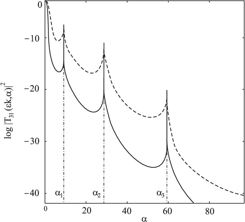
Figure 2: Logarithm of the transmission probability |T31​(ε​k,α)|2|T_{31}(\varepsilon k,\alpha)|^{2} against α\alpha at ε​k=0.0001\varepsilon k=0.0001 (solid curve) and 0.01 (dash curve)
Table 1: Resonant intensities and coupling function
α\alpha θ1​(α)\theta_{1}(\alpha) θ2​(α)=θ3​(α)\theta_{2}(\alpha)=\theta_{3}(\alpha)
8.8104 −0.9992-0.9992 0.02790.0279
28.5513 0.99990.9999 0.00120.0012
59.5701 −0.9999-0.9999 0.997×10−40.997\times 10^{-4}
Table 2: Scattering matrix for α=8.8104\alpha=8.8104
0.9968 −0.0558-0.0558 −0.0558-0.0558
−0.0558-0.0558 −0.9984-0.9984 0.0016
−0.0558-0.0558 0.0016 −0.9984-0.9984
Table 3: Scattering matrix for α=28.5513\alpha=28.5513
0.9996 0.00240.0024 0.00240.0024
0.00240.0024 −0.9999-0.9999 0.288×10−50.288\times 10^{-5}
0.00240.0024 0.288×10−50.288\times 10^{-5} −0.9999-0.9999
Table 4: Scattering matrix for α=59.5701\alpha=59.5701
0.9996 −0.0002-0.0002 −0.0002-0.0002
−0.0002-0.0002 −0.9999-0.9999 0.199×10−70.199\times 10^{-7}
−0.0002-0.0002 0.199×10−70.199\times 10^{-7} −0.9999-0.9999

Since the function QQ vanishes outside the edge ω1\omega_{1}, the resonant set Σ\Sigma coincides with the set Σ1\Sigma_{1} of the simple eigenvalues of (2)–(4). In fact, all eigenfunctions are constant outside the edge ω1\omega_{1} and the resonant set is the spectrum of the problem

−g′′+α​Q​g=0onω1,d​gd​ω1​(a1)=d​gd​ω1​(b)=0.-g^{\prime\prime}+\alpha Qg=0\quad\hbox{on$\quad\omega_{1}$,}\qquad\phantom{-}\frac{dg}{d\omega_{1}}(a_{1})=\frac{dg}{d\omega_{1}}(b)=0.

Table 1 lists the first three positive resonant values of α\alpha (numerically computed using Maple) and the corresponding values of the coupling function θ⁡(α)\theta(\alpha). Tables 2, 3 and 4 list the scattering matrixes for different resonant intensities. We note that the transmission coefficients decay very fast.

The similar effects were observed, when the asymptotic behavior of the scattering coefficients for Hε​(α,Q)\mathrm{H}_{\varepsilon}(\alpha,Q) was discovered directly to the given shape QQ. Figure 2 shows the logarithm of the transmission probability |T31​(ε​k,α)|2|T_{31}(\varepsilon k,\alpha)|^{2} versus α\alpha for ε​k=0.0001\varepsilon k=0.0001 and ε​k=0.01\varepsilon k=0.01. From this figure we see that |T31​(ε​k,α)|2|T_{31}(\varepsilon k,\alpha)|^{2} vanishes as ε→0\varepsilon\to 0 except when α\alpha takes resonant values which correspond to the spikes of |T31​(ε​k,α)|2|T_{31}(\varepsilon k,\alpha)|^{2}. Observe also that the transmission coefficient T31​(ε​k,α)T_{31}(\varepsilon k,\alpha) decays as α→∞\alpha\to\infty.

The author expresses his gratitude to Prof Yu Golovaty for stimulating and helpful discussions.

References

References

  • [1] Albeverio S, Cacciapuoti C and Finco D 2007 J. Math. Phys. 48 032103
  • [2] Albeverio S, Gesztesy F, Høegh-Krohn R and Holden H 2005 Solvable Models in Quantum Mechanics. With an Appendix by Pavel Exner. 2nd revised ed (Providence, RI: AMS Chelsea Publishing) p 488
  • [3] Albeverio S and Kurasov P 1999 Singular perturbations of differential operators: solvable Schrödinger-type operators (Cambridge: Cambridge University Press) p 429
  • [4] Anderson P W 1981 Phys. Rev. B 23 4828
  • [5] Avishai Y and Luck J 1992 Phys. Rev. B 45 1074
  • [6] Chalker J T and Coddington P D 1988 J. Phys. C: Solid State Phys.21 2665
  • [7] Cheon T, Exner P and Turek O 2010 Ann. Phys. 325 548
  • [8] Dell’Antonio G F and Tenuta L 2006 J. Math. Phys. 47 072102
  • [9] Demkov Yu N and Ostrovskii V N 1988 Zero-range potentials and their applications in atomic physics (New York: Plenum) p 240
  • [10] Exner P 1995 Phys. Rev. Lett. 74 3503
  • [11] Exner P 1996 J. Phys. A: Math. Gen.29 87
  • [12] Exner P and Post O 2005 J. Geom. Phys. 54 77
  • [13] Exner P and Šeba P 1989 Rep. Math. Phys. 28 7
  • [14] Flesia C, Johnston R and Kunz H 1987 Europhys. Lett. 3 497
  • [15] Golovaty Yu D and Man’ko S S 2009 Ukr. Math. Bulletin 6 179 (arXiv:0909.1034v1 [math.SP])
  • [16] Golovaty Yu D and Man’ko S S 2009 Dopov. Nats. Akad. Nauk Ukr., Mat. Pryr. Tekh. Nauky 2009, 16
  • [17] Golovaty Yu D and Hryniv R O 2010 J. Phys. A: Math. Gen.43 155204 (arXiv:0911.1046v1 [math.SP])
  • [18] Kostrykin V and Schrader R 1999 J. Phys. A: Math. Gen.32 595
  • [19] Kowal D, Sivan U, Entin-Wohlman O and Imry Y 1990 Phys. Rev. B 42 9009
  • [20] Kuchment P 2002 Waves Random Media 12 R1
  • [21] Man’ko S 2009 Visnyk Lviv Univ.: Mech. Math. 71 142
  • [22] Man’ko S 2010 Visnyk Chernivtsi Univ.: Math. (submitted)
  • [23] Molchanov S and Vainberg B 2007 Comm. Math. Phys. 273 533
  • [24] Pauling L 1936 J. Chem. Phys. 4 673
  • [25] Platt J R 1949 J. Chem. Phys. 17 484
  • [26] Richardson M J and Balazs N L 1972 Ann. Phys. 73 308
  • [27] Šeba P 1986 Rep. Math. Phys. 24 111
  • [28] Christiansen P L, Arnbak H C, Zolotaryuk A V, Ermakov V N and Gaididei Y B 2003 J. Phys. A: Math. Gen.36 7589
  • [29] Zolotaryuk A V, Christiansen P L and Iermakova S V 2006 J. Phys. A: Math. Gen.39 9329
  • [30] Toyama F and Nogami Y 2007 J. Phys. A: Math. Gen.40 F685
  • [31] Zolotaryuk A V 2008 Adv. Sci. Lett. 1 187
  • [32] Zolotaryuk A V 2010 J. Phys. A: Math. Gen.43 105302