Boson stars and oscillatons in an inflationary universe
Abstract
Spherically symmetric gravitationally bound, oscillating scalar lumps (boson stars and oscillatons) are considered in Einstein’s gravity coupled to massive scalar fields in dimensional de Sitter-type inflationary space-times. We show that due to inflation bosons stars and oscillatons lose mass through scalar radiation, but at a rate that is exponentially small when the expansion rate is slow.
I Introduction
Current physical field theories explaining the presently known fundamental interactions are remarkably successful to account for phenomena both on particle physics (i.e. m ) and on cosmological (m) scales, usually incorporate various fundamental scalar fields (Higgs bosons, axion, supersymmetric partners of fermions, inflaton, waterfall fields etc.). It has been observed since a long time ago that self-interacting scalar fields admit at least up to spatial dimensions spatially localized, oscillating lumps, nowadays called oscillons[1, 2, 3]. Oscillons are reminiscent of spatially localized, time-periodic breathers known in one dimensional Sine-Gordon theory. There is, however, a fundamental difference, in that oscillons are only approximatively time-periodic since they radiate, thereby losing continuously their energy, albeit very slowly [4, 5, 6]. Moreover oscillon-type objects exist in a broad class of field theories containing in addition to scalar, vector and possibly other fields [7, 8]. A prominent theory admitting classical oscillons is the bosonic sector of the Standard Model [9, 10, 11]. Einstein’s gravity coupled to a free, massive real Klein-Gordon field, also possesses oscillon-type solutions, which go under the name of oscillatons [12, 13, 14, 15, 16, 17].
An important problem is to investigate the possible pertinence of oscillatons for cosmology where according to current theories some scalars fields are necessarily involved. In recent investigations the evolution of oscillons in an inflating background has been investigated [18, 19, 20, 21, 22, 23]. It has been found that an inflating background also induces a radiative tail in oscillons, distinct from the one present in flat space-times, leading to an additional leakage of energy. However this decay rate is also exponentially suppressed, so inflating oscillons may survive for an exponentially long time provided that the horizon is far larger than the width of an oscillon. As recently shown, due to quantum effects, the decay rate of oscillons becomes power law-like and in many (but not in all) cases dominates over the classical decay rate [24]. There are indications that oscillons can be copiously produced from thermal initial conditions and a substantial fraction of the energy of the system will be stored by them [18, 25, 23]. Therefore it is important to investigate the physical rôle of such long living localized objects. In a cosmological setting it is necessary to take into account the influence of gravity, i.e. instead of simply considering oscillons in a background metric, to investigate solutions of the coupled Einstein-scalar system – oscillatons – with an expanding, asymptotically homogeneous metric.
In this paper we undertake a thorough investigation of localized, oscillaton-type solutions in Einstein’s gravity coupled to a massive Klein-Gordon field, when space-time undergoes inflation, driven by a negative pressure cosmological fluid – i.e. including a cosmological constant, . (For recent reviews on inflation theory see e.g. [26, 27, 28].)
Our results show that once admitting massive scalar fields, both in present day cosmology and in the early Universe, spatially localized, very long living oscillatons exist. The inflaton field generates an energy density of the order of and negative pressure which can be described by an effective (and slowly varying) cosmological parameter. Using the standard slow roll approximation for the inflaton, the metric during the inflationary era can be approximated very well with a de Sitter one. The order of magnitude of the cosmological constant during the inflationary epoch is (in Planck units). If other massive scalar fields are present during inflation such as the waterfall-field in hybrid inflationary scenarios [29, 30], oscillaton production is expected to be significant. We find that oscillatons may survive on cosmological time-scales only if the mass of the scalar field is larger than . The mass loss of an oscillaton during Hubble time is completely determined by the ratio , where is the energy density due to and is that of the oscillaton in its center. For example when the mass loss of such a “waterfall” oscillaton is of the order of during Hubble time. This mass loss is exponentially decreasing for increasing values of the ratio .
Another interesting scenario for oscillaton production is during reheating, assuming that the inflaton field undergoes oscillations near the minimum of its potential. These oscillatons store a considerable amount of energy and due to parametric resonances induced by quantum effects (for oscillons this has been shown in Ref. [24]) they may influence the fluctuation spectrum.
The present value of (in Planck units) being extremely small, its effect on the mass loss of generic oscillatons is completely negligible on a cosmological time scale. For example if the mass of the scalar field is of the order of eV and the amplitude of the oscillaton is approximatively , the effect of the cosmological constant results in a roughly mass loss during the lifetime of the Universe.
We also consider (spherically symmetric) boson stars [31, 32, 33, 34] in this setting, i.e. when a complex scalar field is coupled to gravity with a nonzero cosmological constant. Adopting our small amplitude expansion techniques developed for oscillons and oscillatons we obtain boson star solutions in a systematic way. Remarkably, this method yields very good results even for near maximal mass boson stars. Spatially well localized boson star-type solutions with a static metric, familiar in the case no longer exist when . There exist, however, radiating boson stars with a time dependent metric loosing continually their mass due to emission of scalar waves. We obtain their mass loss using our methods developed for oscillons resp. oscillatons, with the result that this mass loss is exponentially small and it is negligible for sufficiently small values of .
II Field equations
We consider a real or complex scalar field coupled to gravity. The total Lagrangian density is
| (1) |
where the Einstein Lagrangian density in case of a cosmological constant is
| (2) |
We work in a dimensional curved space-time with metric and assume metric signature . Unless explicitly noted, we use Planck units . In some cases it is advantageous to use natural units, where (but ) and all quantities are measured in various powers of electron volts. Because of the different notation in the potential term we consider the real and the complex field case separately. Variation of the action (1) with respect to yields Einstein equations,
| (3) |
II.1 Boson stars
We consider a complex scalar field with a self-interaction potential . For a free field with mass the potential is . The Lagrangian density belonging to the scalar field is
| (4) |
Variation of the action (1) with respect to yields the wave equation
| (5) |
where the prime denotes derivative with respect to . The stress-energy tensor in this case is
| (6) |
We shall assume that the self-interaction potential, , has a minimum at , and expand its derivative as
| (7) |
where is the scalar field mass and are constants.
In order to get rid of the factors in the equations we introduce a rescaled scalar field and potential by
| (8) |
Then
| (9) |
with
| (10) |
II.2 Oscillatons
In this case we consider a real scalar field with a self-interaction potential . For a free field with mass the potential is . The Lagrangian density belonging to the scalar field is
| (11) |
Variation of the action (1) with respect to yields the wave equation
| (12) |
where the prime now denotes derivative with respect to . The stress-energy tensor is
| (13) |
We shall assume that has a minimum at , and expand its derivative as
| (14) |
where is the scalar field mass and are constants.
In order to get rid of the factors in the equations we introduce a rescaled scalar field and potential by
| (15) |
Then
| (16) |
with
| (17) |
II.3 Scaling properties
In both the real and the complex case, if the pair and solves the field equations with a potential and cosmological constant , then
| (18) |
for any positive constant , is a solution with a rescaled potential and rescaled cosmological constant . This scaling property may be used to set the scalar field mass to any prescribed value, for example to make .
If then, by definition, the Einstein tensor is traceless, and from the trace of the Einstein equations it follows that the potential is constant. Hence we assume that .
II.4 Spherically symmetric dimensional space-time
We consider a spherically symmetric dimensional space-time using isotropic coordinates . In this coordinate system the metric is diagonal and its spatial part is in conformally flat form, with components
| (19) |
where and are functions of temporal coordinate and radial coordinate . In case of oscillatons, the periodic change in the acceleration of the constant radius observers is much smaller in isotropic coordinates than in the more commonly used Schwarzschild coordinate system [16, 35]. It is also more convenient to study the Newtonian limit of boson stars using isotropic coordinates [36]. The components of the Einstein tensor are
| (20) | ||||
| (21) | ||||
| (22) | ||||
| (23) |
The potential independent term in the wave equation (5) and (12) is
| (24) |
II.5 de Sitter space-time
If the cosmological constant is positive, far from the central boson star or oscillaton the space-time should approach the de Sitter metric. In static Schwarzschild coordinates on a dimensional space-time this metric can be written as
| (25) |
where is the metric on the unit sphere . The Hubble constant is related to the cosmological constant by
| (26) |
In isotropic coordinates the de Sitter metric takes the form
| (27) |
where the two radial coordinates are related by
| (28) |
The cosmological horizon, which is at in the Schwarzschild coordinate system, is at in isotropic coordinates.
III Small-amplitude expansion
The small-amplitude expansion procedure has been applied successfully to describe the core region of flat background oscillons [1, 4, 37, 38]. The method was generalized in [35] to the case when the scalar field is coupled to Einstein gravity, and in [39] to a very similarly behaving scalar-dilaton system. In this section we expand oscillatons in the case when the cosmological constant is positive.
Newtonian boson stars have already been investigated in the paper of Ruffini and S. Bonazzola [32], obtaining a system of two coupled differential equations, which nowadays are generally called Schrödinger-Newton equations in the literature[40, 41, 42, 43]. The same system was obtained as weak gravity limit of general relativistic boson stars in [44] and [45]. The leading order results of the small-amplitude expansion of boson stars, that we present in this section, when restricted for , also yield the same equations.
The repulsive effect of the cosmological constant is taken into account in a similar way as in [20, 21, 22]. Since we intend to investigate localized objects, where at large distances the scalar field is negligible, by the generalized Birkhoff’s theorem [46, 48, 47], the metric should approach the Schwarzschild-de Sitter metric. This also means that in the asymptotic de Sitter region the expansion rate (Hubble parameter) is constant.
III.1 Choice of coordinates
We are looking for spatially localized bounded solutions of the field equations for which is small and the metric is close to de Sitter. The smaller the amplitude of a boson star or an oscillaton is, the larger its spatial extent becomes. Therefore, we introduce a new radial coordinate by
| (29) |
where denotes the small-amplitude parameter. Motivated by the scaling property (18) we have also included a factor into the definition of .
Long-living localized solutions are expected to exist only if their size is considerably smaller than the distance to the cosmological horizon. We introduce a rescaled Hubble constant by
| (30) |
and assume that even is reasonably small. This way we ensure that the typical size of boson stars or oscillatons, which is of the order using the coordinates, remains smaller than the radius of the cosmological horizon, .
We will see in Section III.5 that the energy density of the scalar field at the central region of small amplitude oscillons or boson stars is proportional to . On the other hand, the cosmological constant can be interpreted as a fluid with energy density,
| (31) |
and pressure . Using (26) and (30) can be written as
| (32) |
The smallness of guaranties that remains smaller than energy density of the scalar field even in the small-amplitude limit.
We expand and the metric functions in powers of as
| (33) | ||||
| (34) | ||||
| (35) |
The first terms in and represent the de Sitter background, according to (27). Since we intend to use asymptotically de Sitter coordinates, we look for functions , and that tend to zero when is large. One could initially include odd powers of into the expansions (33)-(35). However, for oscillatons it can be shown by the method presented below, that the coefficients of those terms necessarily vanish when we are looking for configurations that remain bounded in time. It can also be verified directly, that the small-amplitude expansion of boson stars do not include odd powers of . This is in contrast to flat background oscillons, where the leading order behavior of the amplitude is proportional to .
The frequency of boson stars and oscillatons also depends on their amplitude. The smaller the amplitude is, the closer the frequency becomes to the threshold . Hence we introduce a rescaled time coordinate by
| (36) |
and expand the square of the dependent factor as
| (37) |
It is possible to allow odd powers of into the expansion of , but the coefficients of those terms turn out to be zero when solving the equations arising from the small-amplitude expansion. There is a considerable freedom in choosing different parametrizations of the small-amplitude states, changing the actual form of the function . The physical parameter is not but the frequency of the periodic states that will be given by . Similarly to the asymptotically flat case in [35] and to the dilaton model in [39], it turns out that for spatial dimensions the parametrization of the small-amplitude states can be fixed by setting .
The field equations we intend to solve using the and coordinates are the Einstein equations (3), substituting the Einstein tensor components from (20)-(23), together with the wave equation (5) or (12). We note that these equations are not independent. The component of the Einstein equations is a constraint, and the wave equation is a consequence of the contracted Bianchi identity.
III.2 Boson stars
In case of boson stars the metric is static, hence and are time independent. The complex scalar field oscillates with frequency ,
| (38) |
where is real and depends only on the radial coordinate . The small-amplitude expansion coefficients of satisfy
| (39) |
where are real functions of . Substituting the expansion (33)-(35) into the field equations, if , then to leading order the component gives
| (40) |
Since for there is no solution representing a localized object we assume . Then the component and the wave equation yield to leading order a coupled system of differential equations for and ,
| (41) | ||||
| (42) |
Introducing the functions and by
| (43) |
equations (41) and (42) can be written into the form
| (44) | ||||
| (45) |
Since the same equations will be obtained for small-amplitude oscillatons in the next subsection, we postpone the discussion of this system to Subsection III.4.
Proceeding to higher orders, the components give a system of lengthy differential equations linear in , , and their derivatives. These equations have nonlinear source terms containing , and . They will also involve the first coefficient from the series expansion of the potential . To leading order, the structure of small-amplitude boson stars only depends on the mass parameter .
III.3 Oscillatons
In this case the scalar field is real, and the metric components are also oscillating. We are looking for solutions that remain bounded as time passes. It turns out, that these configurations are necessarily periodically oscillating in time.
From the components of the field equations follows that only depends on and that
| (46) |
where two new functions, and are introduced, depending only on . From the part of the component of the Einstein equations it follows that can remain bounded as time passes only if is a constant. Then by a shift in the time coordinate we set
| (47) |
This shows that the scalar field oscillates simultaneously, with the same phase at all radii.
From the component of the difference of the and Einstein equations follows that also depends only on the radial coordinate , showing that the metric is static to order . This is the main advantage of using isotropic coordinates over Schwarzschild coordinates. But even in this system the coefficients and will already contain terms. From the component of the Einstein equations follows that
| (48) |
where is a function of . The component shows that if then
| (49) |
If then , and there are no nontrivial localized regular solutions for and , so we assume from now. The component yields
| (50) |
The wave equation provides an equation that determines the time dependence of . In order to keep bounded, the resonance terms proportional to must vanish, yielding
| (51) |
III.4 Schrödinger-Newton equations
The equations describing both small-amplitude boson stars and oscillatons on an expanding background has been written into a form, which for reduces to the time-independent Schrödinger-Newton (SN) equations [40, 41, 42, 43]
| (53) | ||||
| (54) |
If and are solutions of (53) and (54), then the transformed functions
| (55) |
solve the equations
| (56) | ||||
| (57) |
which are obtained from the SN equations by replacing the constant by .
If the scalar field, and consequently , tends to zero for then (54) gives the following approximation for ,
| (58) |
Since we are looking for solutions for which also approaches zero for large , necessarily . In order to make the solution of the SN equations (53)-(54) unique we demand
| (59) |
Setting for this also fixes the connection between the frequency and the small-amplitude parameter , giving
| (60) |
III.5 Energy density
The energy density of the scalar field is , where the unit timelike vector has the components . In terms of the rescaled scalar field , the energy density of oscillatons can be written as
| (62) |
and for boson stars
| (63) |
In case of boson stars, using (33), (39) and (43), to leading order in we get
| (64) |
For oscillatons we obtain the same expression for using (33), (46) and (52). Measuring the scalar field mass in units, the energy density at the symmetry center for can be written as
| (65) |
(We use Roman for meters in order to distinguish from the scalar field mass .) Here we have used the numerically obtained central value of , which is for .
The effective energy density corresponding to the present value of the cosmological constant is given in ordinary units by (180) in Appendix D. Comparing to (65), one can see that the energy density of the scalar field is much higher than unless or is extremely small. Using (32), the ratio of to the central density can be written as
| (66) |
providing an important physical interpretation for the rescaled Hubble constant . In Table 1 we give the value of and the coefficient of in for the relevant dimensions.
We will see in the following sections that turns out to be the essential parameter determining the energy loss rate of boson stars and oscillatons.
III.6 Outer core region
If , and the cosmological constant is zero, i.e. , then assuming that the SN equations have a unique localized nodeless solution. Solutions with nodes have higher energy and are unstable. For large the function satisfies the equation
| (67) |
which has exponentially decaying solutions
| (68) | ||||||
| (69) |
The numerically determined values of the constants and for the case are given in Table 2.
Even if is nonzero, we assume that it is small enough such that there is a region of which is well outside the core region, but where the influence of the cosmological constant is still negligible. In this region satisfies (67), and consequently (68) and (69) are good approximations together with the values of the constants belonging to the case given in Table 2.
III.7 Oscillating tail region
If is nonzero, at very large distances , and the behavior of is determined by the equation
| (70) |
The function has an oscillating standing wave tail in this domain,
| (71) |
where and are constants, describing the amplitude and phase. We can interpret this standing wave as the superposition of an outgoing wave carrying energy out from the central object and an artificial ingoing wave component that is added to keep the solution exactly periodic. We will relate the amplitude of the tail to the energy loss rate of dynamical boson stars or oscillatons.
When solving the SN equations (53) and (54) by a numerical method, the amplitude depends on the central values of and given at . We intend to determine the minimal tail amplitude, , assuming that tends to for . We are interested in solutions which has no nodes in the central region where the influence of is negligible. If then is nonzero. In order to show the influence of on the form of the function , on Fig. 1 we plot the radial dependence of for and for .

Assuming that is small, we calculate the amplitude by WKB analysis. Our aim is to continue the function given by (68) and (69) into the very large distances where the cosmological term dominates. We will express the amplitude in terms of the constant . To the function which is exponentially decaying when going outwards at the outer core region belongs an oscillating tail with a certain amplitude and phase. Adding the mode which exponentially grows when going outwards does not change the function noticeably in the outer core region but adds an oscillating tail with a phase shift . The resulting tail amplitude is minimal if this second mode is not present. Hence the WKB method will give the minimum amplitude . In Sec. IV.6 we will compare the WKB amplitude to results obtained by direct numerical integration of the SN equations. Besides indicating the correctness of the WKB results, this will also give information on how large can be chosen such that the WKB result can be still considered a valid approximation.
IV WKB formalism
IV.1 Schrödinger form
Introducing a new radial coordinate
| (72) |
we transform (61) into a form corresponding to a Schrödinger equation with playing the role of the Planck’s constant ,
| (73) |
Introducing
| (74) |
we can transform this into a one-dimensional form,
| (75) |
where
| (76) |
The outer domain of the core region is represented now by , where
| (77) | ||||||
| (78) |
IV.2 WKB approximation
Introducing a new function by
| (79) |
and substituting into (75) we get
| (80) |
We write f as a power series in ,
| (81) |
Differently from the standard WKB approach, now also has to be expanded in ,
| (82) |
where the nonvanishing coefficients are
| (83) | ||||
| (84) | ||||
| (85) |
Substituting into (80), to leading order we get
| (86) |
The order components yield
| (87) |
IV.3 WKB for
If then ,
| (88) |
and we get the standard WKB result,
| (89) | ||||||
| (90) |
The general solution for is a sum of two terms with proportionality constants and , and similarly for the case with constants and . For the case . Substituting (83), it is possible to perform the integral in the exponentials. For ,
| (91) |
while for ,
| (92) |
In the region , substituting the expansion of (91), to leading order (89) takes the form
| (93) |
Comparing with (78), follows that for
| (94) |
IV.4 WKB for
IV.5 Connection formulae
The next step is to relate the amplitudes in the region to the amplitudes for . The expressions (89) and (90) for are just the standard WKB solutions, so one can apply the appropriate connection formulae to express in terms of . In our case we need the one where the field is exponentially increases when going away from the turning point (see for example (34.18) of [49])
| (103) |
from to . This is equivalent to
| (104) |
The expressions (99) and (100) for differ from the standard WKB solutions by factors involving . However, since both of these factors take the value at the turning point, the formulae (104) relating the amplitudes at the two sides hold in this case too. A detailed derivation of (104) is given in Appendix A.
IV.6 Schrödinger-Newton tail amplitude
For the expression (92) can be approximated by
| (105) |
In the case to leading order (90) yields
| (106) |
Substituting from (104) gives
| (107) |
For , to leading order (100) yields
| (108) |
and substituting from (104) gives
| (109) |
Using (74) we can express the original variable in the SN equations using the coordinate , obtaining the same asymptotic formula as in (71),
| (110) |
where the amplitude is
| (111) |
for any , and the phase is
| (112) |
Substituting the value of from (94) and (102) gives our final WKB result for the minimal amplitude
| (113) |
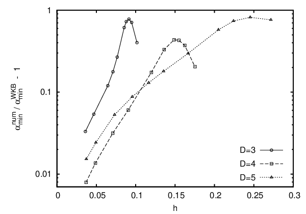
It is instructive to compare the above analytical result to the minimal amplitude obtained by the numerical solution of the SN equations (53)-(54). For a chosen one has to minimize the oscillating tail for those solutions for which the field tends to asymptotically, while has no nodes in the core region. The solutions depend very strongly on the central values and . The results for various for spatial dimensions are listed in Table 3.
The amplitudes for dimensions are plotted on Fig. 2, and the relative difference from the analytically obtained WKB value is displayed on Fig. 3.

From this figure we read off that the WKB analysis gives less than error, if in case of , and if when or .
IV.7 Scalar field tail amplitude
For oscillatons, using (33), (46), (52) and (110), the real scalar in the tail region behaves like
| (114) |
where the amplitude is
| (115) |
Applying the identity
| (116) |
it is apparent that (114) is a sum of an ingoing and outgoing wave, both with amplitude . One might be tempted to add an ingoing wave with an opposite amplitude to obtain a purely outgoing solution, and to conclude that the remaining outgoing component has the amplitude . However, an ingoing wave contains a component, which would change the amplitude of the WKB mode which is increasing when going away from the turning point. What one can do instead is adding a standing wave proportional to , corresponding to the suppressed WKB mode. If the time dependence is also phase shifted, then we obtain the minimal amplitude outgoing wave,
| (117) |
IV.8 Mass loss rate
Even if in the oscillating tail region, according to (34) and (35), for small the metric functions and are still very close to . The mass loss rate of the system can be calculated by applying the expression (165) for the time derivative of the mass function from Appendix B,
| (121) |
Substituting the stress energy tensor from (6) or (13),
| (122) |
which expression is valid for both real and complex fields. We have to evaluate this expression at large in the tail region. Substituting the outgoing wave form (117) and averaging for one oscillation period, or substituting (120), for both the oscillaton and boson star case we obtain
| (123) |
Here, since we are interested in the leading order result, we substituted , and for large we neglected the term arising when taking the derivative of the factor. For large radius agrees with the total mass of the oscillon or boson star. Using (113) and (115) for the mass loss rate and substituting , for we obtain
| (124) |
If there is an extra term involving ,
| (125) |
For small-amplitude configurations the parameter can be expressed by the mass using (168). Because of the complexity of the resulting expression we only give the result for , when
| (126) |
For specific and this can be integrated numerically in order to obtain the change of the mass as a function of time.
Using the leading order expression (168) for the total mass and dividing by we can obtain the the relative mass loss rate. The Hubble time describes the time-scale of the expansion of the universe. The value of obtained from the present value of the cosmological constant is given by (184) in Appendix D. Dividing by both and we obtain the relative mass loss extrapolated for a period corresponding to the Hubble time. For ,
| (127) |
and for ,
| (128) |
where the values of the constants , are given in Table 2. This result is independent on the units used to measure the time and mass, and it depends on , and only through the rescaled cosmological constant . According to (66) the square of the parameter is proportional to the ratio of the central density to the effective energy density corresponding to the cosmological constant . On fig. 4 and on Table 4 we give as a function of the density ratio .

V Mass loss rate of oscillatons in the case
If the cosmological constant is zero and the space-time is asymptotically flat then the metric of boson stars is static and their mass is independent of time. In contrast, oscillatons are very slowly losing mass by scalar field radiation even in the case [16]. This mass loss is nonperturbatively small in the amplitude parameter . According to [35], for this mass loss rate depends only on the amplitude parameter, and it is given by
| (129) |
where the numerical values of the constants are
| (130) |
For small this is exponentially small, while the mass loss induced by the cosmological constant, given by (125), tends to zero only polynomially when . This implies that if then for small the mass loss (125) originating from the cosmological constant dominates, while for large the expression (129) can be applied. Apart from the amplitude parameter the mass loss (125) depends only on the ratio . It can be checked numerically that for a concrete choice of there is only one value where the two type of mass loss rates are equal, which we denote by . For low values the function can be expanded as
| (131) |
with
| (132) |
| (133) |
where the newly introduced two constants are
| (134) |
On Fig. 5 we plot as a function of . To illustrate how well the above analytic approximation works we plot for relatively large values of , although the solutions for are unstable.

The quantity is originally assumed to be in Planck units, but it has the same simple form in natural units if the Hubble constant is expressed in electron volts.
VI Possible effects in the current universe
From the definition (30) of the rescaled cosmological constant we can express the square of the small-amplitude parameter . The amplitude of the scalar field is proportional to to leading order. Measuring the cosmological constant in units and the scalar field mass in units, (30) can be written as
| (135) |
According to (127) and (128), the part of the mass lost during a Hubble time period only depends on the value of the rescaled Hubble constant . For example, we can look for configurations where this mass loss is one percent. According to Table 4, for the physically interesting dimensional case this corresponds to the value of . Using the present value of the Hubble constant, which is given by (183),
| (136) |
Oscillatons or boson stars are generally stable if the amplitude parameter , which for larger amplitudes can be defined from the frequency by is smaller than . From (136) it is apparent that significant mass loss for the larger amplitude configurations with can happen only for extremely small scalar field masses. Very small values are not excluded, but since for , according to (170), the total mass of the oscillaton or boson star is proportional to , these configurations tend to have extremely small masses. Similarly, since by (176) the radius is inversely proportional to , small values belong to spatially extended configurations. It is obvious that the influence of the cosmological constant is larger for large radius objects. In Table 5 we list the values of , the total mass and the radius for various choices of the scalar field mass , assuming that the mass-loss extrapolated for a Hubble time period is .
Keeping the same scalar mass, for larger , and consequently, for larger total masses and smaller radiuses, the mass loss rate is smaller than . For all configurations listed in Table 5 the oscillaton mass loss rate given by (129) is negligible, many orders of magnitude smaller than .
To show some concrete examples, we examine three specific choices for the scalar field mass. Firstly, for an axion with the mass of the oscillaton for which is about that of a very small asteroid, and its radius is about astronomical units. Secondly, if , then the total mass is about a solar mass, , which is distributed in a region of radius of light-years. Thirdly, for the corresponding mass is about the mass of the Milky Way (including dark matter), and the radius is light-years, which is about four times the radius of the stellar disk. According to Table 4 and (180), for all the above configurations the central density is .
The maximal amplitude boson stars or oscillatons, with generally have much bigger masses and smaller sizes than the states with mass loss discussed in the previous paragraphs. For example, the oscillaton for the axion case has a mass (about four Earth masses) and radius . Only considering the mass loss (125) induced by the cosmological constant, the maximal amplitude boson stars or oscillatons have extremely long lifetime. For the axion case, using (135), we get , and the relative mass loss during a Hubble time period is of the order , certainly negligible. For boson stars formed by complex fields this is the only mechanism to lose mass, consequently, close to maximal mass boson stars have practically constant mass. However oscillatons lose mass even in the case by (129) which gives for , showing that this state is unstable on the cosmological time-scale. However, the mass loss decreases exponentially with . An initially maximal mass oscillaton created in the early universe loses mass relatively quickly, and its amplitude parameter decreases to about during a Hubble time period, where according to (129) the relative mass loss rate is . For more details and different scalar field masses see Table VIII of [35].
VII Inflationary era
The energy density of the inflaton field during the inflationary epoch can be estimated as (see e.g. [26]). This expression is valid in natural units, where (but ) and the energy is measured in electron volts. In ordinary units this corresponds to the mass density . Assuming a de Sitter geometry, the Hubble constant is
| (137) |
in ordinary and natural units. By (26) this belongs to a cosmological constant
| (138) |
in ordinary and Planck units, respectively.
If in addition to the inflaton field there is another scalar field on this de Sitter background, and it is massive, then it is likely to form localized oscillaton configurations (or boson stars in case of a complex field). This second field may be, for example, the waterfall field in a hybrid inflation theory[29, 30]. If the mass parameter of the field is , then we can apply (135) to relate the small-amplitude parameter to the rescaled Hubble constant . The parameter is the essential parameter determining the mass loss rate of the object. For example, if the mass loss extrapolated for a Hubble time period is assumed to be , then , and for the inflationary era we obtain
| (139) |
Since oscillatons and boson stars are stable only if the amplitude parameter satisfies , states with mass loss can only exist for . For objects formed from fields with , necessarily . Then from (135) it follows that , which implies that the mass loss during the Hubble time is always larger than . Oscillatons and boson stars formed from scalar fields with mass are very short living during the inflationary era. Another way to see why this lower limit is necessary is to calculate the central density by (65), and observe that for small scalar field mass , and hence long living oscillatons are not expected to exist.
For scalar field masses we list the properties of some oscillatons with mass loss in Table 6.
All these states have the central density , and the mass loss is much smaller than for them.
The mass loss rate induced by the cosmological constant decreases very quickly when considering higher amplitude configurations. The behavior of the oscillaton mass loss is just the opposite. The two kind of relative mass loss extrapolated for a Hubble time period of some maximal amplitude states belonging to are given in Table 7.
VIII Reheating
Oscillatons are likely to form after the end of inflation, in the reheating era, when the inflaton field is oscillating around the potential minimum. These oscillatons are likely to influence the efficiency of how the inflaton’s energy is transferred to other fields. Since oscillatons are concentrated energy lumps, their influence on the formation of inhomogeneities may also be important. At the reheating stage the equation of state can be well approximated by a pressureless fluid, and hence the effective cosmological constant can be taken to be zero. For the lifetime of oscillatons in this era one can apply the considerations given in [35] which are valid in the asymptotically flat case. The mass of the inflaton field when it is near the vacuum value can be estimated as (see e.g. [28]). The maximal amplitude stable oscillaton which can be formed by this field, when , has the total mass and radius . The mass and radius of smaller amplitude oscillatons formed by this field can be easily obtained by using the fact that the total mass is proportional to and the radius is proportional to .
If the cosmological constant is zero, then a natural time scale is the oscillation period, . According to (60), for small we can replace by . Taking the total mass from (169), the part of the mass lost during an oscillation period is
| (140) |
This expression is independent of the scalar field mass and on the units that we use for measuring time. Even for the maximal amplitude oscillaton with this gives a very tiny value, . This shows that oscillatons formed in the reheating period perform a large number of oscillations before the mass loss by emitting classical scalar field radiation becomes apparent. However, since their oscillation period is extremely short, , they lose about half of their mass in . On the other hand, since this mass loss depends exponentially on , even during a period corresponding to the lifetime of the universe the amplitude parameter does not decrease much below , where .
IX Conclusions
We have constructed spherically symmetric, spatially localized time dependent solutions in a large class of scalar theories coupled to Einstein’s theory of gravitation and a positive cosmological constant, . Examples include boson star-type objects (for a complex field) and oscillatons (for a real field), considered previously for vanishing cosmological constant. A positive constant has important qualitative effects on boson stars, in that due to the repulsion induced by only radiating solutions exist, leading to a mass loss. For sufficiently small values of this effect is negligible, so boson stars with almost unchanged mass may be present in our Universe. Even when oscillatons radiate slowly, and the consequent mass loss is maximal for large amplitudes. There is an additional mass loss of oscillatons induced by a nonzero , which dominates for small amplitudes (corresponding to large sizes). The mass loss of an oscillaton during a Hubble time period, is completely determined by the ratio , where is the energy density due to and is that of the oscillaton in its center. Our computations are valid in spatial dimensions , although the case has been given special attention. An important cosmological application of our results is for ”waterfall”-type oscillatons appearing in hybrid inflation models.
Appendix A Connection formulae
In this appendix we derive the formulae (104) connecting the amplitudes in the and regions. We follow the method described in [50]. Since the expressions for obtained by the WKB method are singular at , it is necessary to find a solution of (75) which is valid in a region around this point. Let us introduce a new radial coordinate by
| (141) |
We approximate for small by
| (142) |
Introducing a rescaled coordinate by
| (143) |
(75) takes the form
| (144) |
The solution can be written in terms of Airy functions
| (145) |
For this has the asymptotic form
| (146) |
and for
| (147) |
We consider two matching regions surrounding , where and at the same time . Both of these can hold simultaneously if is small enough. First we continue through the matching region with . Substituting into (91) and expanding in power series around , we obtain
| (148) |
This result can also be obtained by simply approximating by . In this region the influence of the term is subleading, so for dimensions we obtain both from (89) and (99)
| (149) |
Comparing with (146), we get
| (150) |
Appendix B Mass in spherically symmetric asymptotically de Sitter space-times
Since the scalar field tends to zero exponentially, at large distances the metric approaches the static Schwarzschild-de Sitter metric. Considering dimensional space-times, in Schwarzschild area coordinates the Schwarzschild-de Sitter metric has the form
| (155) |
where
| (156) |
and is a constant related to the mass by
| (157) |
In general spherically symmetric space-times there is a naturally defined radius function , defined in terms of the area of the symmetry spheres. In Schwarzschild coordinates , while in the isotropic coordinates (19) . In terms of this radius function one can define the Misner-Sharp energy (or local mass) function [51, 52], which can be defined for arbitrary dimensions by
| (158) |
For the Schwarzschild-de Sitter metric . At infinity the mass function agrees with the Abbott-Deser mass [53, 54], which is a Killing energy defined in static asymptotically de Sitter space-times.
The Misner-Sharp energy also agrees with a conserved energy that can be defined using the Kodama vector. The Kodama vector [55, 56] is defined by
| (159) |
where is the volume form in the plane. Choosing the orientation such that makes future pointing, with nonvanishing components
| (160) |
It can be checked that, in general, the Kodama vector is divergence free, . Since contracting with the Einstein tensor, , the current
| (161) |
is also divergence free, , it defines a conserved charge. Integrating on a constant hypersurface with a future oriented unit normal vector , the conserved charge is
| (162) | ||||
It can be checked that the derivative of the mass function can be expressed in terms of the current ,
| (163) |
For the radial derivative follows that
| (164) |
which, comparing with (162), gives .
The time derivative of the mass function is
| (165) |
This equation describes the mass loss caused by the outward energy current of the massive scalar field.
For large radii the function tends to the total mass of the oscillon or boson star. Substituting the small-amplitude expansions (34) and (35) into the definition (158) of the mass function , to leading order in we obtain
| (166) |
We have seen in Subsections III.2 and III.3 that for both the boson star and oscillaton case and , giving
| (167) |
Since the asymptotic behavior of is given by (58),
| (168) |
For dimensional space-time
| (169) |
For small the numerical value of the constant can be approximated by the value given in Table 2. Measuring the belonging to the scalar field in electron volts and the mass of the boson star or oscillaton in kilograms,
| (170) |
Appendix C Proper mass and core radius
The proper mass inside a sphere of radius is defined by the dimensional volume integral of the energy density ,
| (171) |
Substituting the leading order expression (64) for , and the leading order value from (35), using the rescaled radial coordinate ,
| (172) |
The integral can be performed using the SN equation (54),
| (173) |
To leading order in the calculated proper mass agrees with the mass function given by (167). However at higher order the proper mass is expected to be larger by an amount corresponding to the binding energy.
Oscillatons and boson stars do not have a definite outer surface. A natural definition for their size is to take the radius inside which percentage of the mass-energy can be found. It is usual to take, for example, or . The mass-energy inside a given radius can be defined either by the integral (171) or by taking the local mass function in (158). To leading order in both definitions give (173). The rescaled radius can be defined by
| (174) |
The numerical values of for various in dimensions are listed in Table 8.
The physical radius is
| (175) |
In ordinary units, measuring the scalar field in electron volts and in meters (Roman ),
| (176) |
We note that for complex field boson stars the current
| (177) |
can be used to define a conserved quantity. The conserved particle number can be defined by integrating the time component for a spacelike slice. To leading order in the function is proportional to the density given in (64). Hence, to this order, the use of the particle number instead of the mass-energy yields the same result for the radius of boson stars.
Appendix D Present value of the cosmological constant
For the present observational value of the Hubble constant we take
| (178) |
according to the combined 7-year WMAP data [57]. To this corresponds a critical density
| (179) |
The fraction of this belonging to the dark energy provided by the cosmological constant is given by , according to WMAP results [57]. Consequently, the energy density belonging to the cosmological constant is
| (180) |
According to (31), this corresponds to a cosmological constant of
| (181) |
In Planck units, since the Planck length is ,
| (182) |
Since we are interested in the effect of the cosmological constant, we neglect the ordinary and dark matter content of the universe. Then the space-time can be described by a de Sitter metric with Hubble constant given by (26). In Planck, ordinary and natural units
| (183) |
The Hubble time is then
| (184) |
Even though the ordinary and dark matter content have been neglected, this value is still not too far from the age of the universe, which according to WMAP data is assuming the model [57].
Acknowledgements.
This research has been supported by OTKA Grants No. K61636, NI68228, and by the U.S. Department of Energy (D.O.E.) under cooperative research agreement DE-FG 0205ER41360.References
- [1] R. F. Dashen, B. Hasslacher and A. Neveu, Phys. Rev. D 11, 3424 (1975).
- [2] I. L. Bogolyubskii, and V. G. Makhan’kov, JETP Letters 25, 107 (1977).
- [3] E. J. Copeland, M. Gleiser and H.-R. Müller, Phys. Rev. D 52, 1920 (1995).
- [4] H. Segur and M. D. Kruskal, Phys. Rev. Lett. 58, 747 (1987).
- [5] G. Fodor, P. Forgács, Z. Horváth and M. Mezei, Phys. Rev. D 79, 065002 (2009).
- [6] G. Fodor, P. Forgács, Z. Horváth and M. Mezei, Phys. Lett. B 674, 319-324 (2009).
- [7] M. Gleiser and J. Thorarinson, Phys. Rev. D76, 041701(R) (2007).
- [8] M. Gleiser and J. Thorarinson, Phys. Rev. D79, 025016 (2009).
- [9] E. Farhi, N. Graham, V. Khemani, R. Markov and R. Rosales, Phys. Rev. D 72, 101701(R) (2005).
- [10] N. Graham Phys. Rev. Lett. 98, 101801 (2007).
- [11] N. Graham Phys. Rev. D 76, 085017 (2007).
- [12] E. Seidel and W-M. Suen, Phys. Rev. Lett. 66, 1659 (1991).
- [13] E. Seidel and W-M. Suen, Phys. Rev. Lett. 72, 2516 (1994).
- [14] L. A. Ureña-López, T. Matos and R. Becerril, Class. Quantum Grav. 19, 6259 (2002).
- [15] M. Alcubierre, R. Becerril, F. S. Guzmán, T. Matos, D. Núñez and L. A. Ureña-López, Class. Quantum Grav. 20. 2883 (2003).
- [16] D. N. Page, Phys. Rev. D 70, 023002 (2004).
- [17] J. Balakrishna, R. Bondarescu, G. Daues and M. Bondarescu, Phys. Rev. D 77, 024028 (2008).
- [18] M. Broadhead and J. McDonald, Phys. Rev. D 72, 043519 (2005).
- [19] M. Gleiser. Int. J. Mod. Phys. D 16, 219 (2007).
- [20] N. Graham and N. Stamatopoulos, Phys. Lett. B639, 541 (2006).
- [21] E. Farhi, N. Graham, A. H. Guth, N. Iqbal, R. R. Rosales and N. Stamatopoulos, Phys. Rev. D 77, 085019 (2008).
- [22] M. A. Amin and D. Shirokoff, Phys. Rev. D 81, 085045 (2010).
- [23] M. A. Amin, arXiv:1006.3075 [astro-ph.CO] (2009).
- [24] M. P. Hertzberg, arXiv:1003.3459 [hep-th] (2010).
- [25] M. Gleiser, N. Graham and N. Stamatopoulos, arXiv:1004.4658 [astro-ph.CO] (2010).
- [26] D. H. Lyth and A. R. Liddle, The Primordial Density Perturbation, Cambridge (2009).
- [27] S. Weinberg, Cosmology, Oxford (2008).
- [28] V. Mukhanov, Physical Foundations of Cosmology, Cambridge (2005).
- [29] A. D. Linde, Phys. Lett. B 259, 38 (1991)
- [30] A. D. Linde, Phys. Rev. D 49, 748 (1994)
- [31] D. J. Kaup, Phys. Rev. 172, 1331 (1968).
- [32] R. Ruffini and S. Bonazzola, Phys. Rev. 187, 1767 (1969).
- [33] P. Jetzer, Phys. Rep. 220, 163 (1992).
- [34] F. E. Schunk and E. W. Mielke, Class. Quantum Grav. 20, R301 (2003).
- [35] G. Fodor, P. Forgács and M. Mezei, Phys. Rev. D 81, 064029 (2010).
- [36] R. Friedberg, T. D. Lee and Y. Pang, Phys. Rev. D 35, 3640 (1987).
- [37] S. Kichenassamy, Comm. Pur. Appl. Math. 44, 789 (1991).
- [38] G. Fodor, P. Forgács, Z. Horváth and Á. Lukács, Phys. Rev. D 78, 025003 (2008).
- [39] G. Fodor, P. Forgács, Z. Horváth and M. Mezei, JHEP08(2009)106, (2009).
- [40] L. Diósi, Phys. Lett. A 199. 105 (1984).
- [41] R. Penrose, Phil. Trans. R. Soc. 356. 1 (1998).
- [42] I. M. Moroz, R. Penrose and P. Tod, Class. Quantum Grav. 15, 2733 (1998).
- [43] P. Tod and I. M. Moroz, Nonlinearity 12, 201 (1999).
- [44] R. Friedberg, T. D. Lee, and Y. Pang, Phys. Rev. D 35, 3640 (1987).
- [45] R. Ferrell and M. Gleiser, Phys. Rev. D 40, 2524 (1989).
- [46] J. Eiesland, Transactions of the American Mathematical Society 27, 213 (1925).
- [47] K. Schleich and D. M. Witt, arXiv:0908.4110 [gr-qc] (2009).
- [48] J. Morrow-Jones and D. M. Witt, Phys. Rev. D 48, 2516 (1993).
- [49] L. I. Schiff, Quantum Mechanics, Third Edition, (McGraw-Hill, 1968)
- [50] D. J. Griffiths, Introduction to Quantum Mechanics, (Prentice Hall, New Jersey, 1995)
- [51] C. W. Misner and D. H. Sharp, Phys. Rev. 136, B571 (1974).
- [52] K. Nakao, arXiv:gr-qc/9507022 (1995)
- [53] L. Abbott and S. Deser, Nucl. Phys. B 195, 76 (1982).
- [54] K. Nakao, T. Shiromizu and K. Maeda, Class. Quantum Grav. 11, 2059 (1994).
- [55] H. Kodama, Prog. Theor. Phys 63, 1217 (1980).
- [56] S. A. Hayward, Phys. Rev. D 53, 1938 (1996).
- [57] E. Komatsu at al., arXiv:1001.4538 [astro-ph.CO] (2010).