跳到论文正文
W Papers独立论文阅读器 arXiv:1007.0199 论文正文 计算阅读时间 · 0%
引用这篇论文根据当前论文元数据生成,正式投稿前建议核对。


License: arXiv.org perpetual non-exclusive license
arXiv:1007.0199v5 [q-fin.TR] 24 Aug 2011

optimal execution strategy in the presence of permanent price impact and fixed transaction cost

Mauricio Junca ††thanks: Department of Industrial Engineering and Operations Research, University of California, Berkeley CA 94720-1777. Email address: mjunca@berkeley.edu
Abstract

We study a single risky financial asset model subject to price impact and transaction cost over an infinite horizon. An investor needs to execute a long position in the asset affecting the price of the asset and possibly incurring in fixed transaction cost. The objective is to maximize the discounted revenue obtained by this transaction. This problem is formulated first as an impulse control problem and we characterize the value function using the viscosity solutions framework. We also analyze the case where there is no transaction cost and how this formulation relates with a singular control problem. A viscosity solution characterization is provided in this case as well. We also establish a connection between both formulations with zero fixed transaction cost. Numerical examples with different types of price impact conclude the discussion.

Keywords: Price impact, impulse control, singular control, dynamic programming, viscosity solutions

1 Introduction

An important problem for stock traders is to unwind large block orders of shares. Market microstructure literature has shown (e.g. (Chan and Lakonishok, 1995; Holthausen et al., 1990)), both theoretically and empirically, that large trades move the price of risky securities either for informational or liquidity reasons. Several papers addressed this issue and formulated a hedging and arbitrage pricing theory for large investors under competitive markets. For example, in (Cvitanić and Ma, 1996) a forward-backward SDE is defined, with the price process being the forward component and the wealth process of the investor’s portfolio being the backward component. In both cases, the drift and volatility coefficients depend upon the price of the stocks, the wealth of the portfolio and the portfolio itself. (Frey, 1998) describes the discounted stock price using a reaction function that depends on the position of the large trader. In (Bank and Baum, 2004; Çetin et al., 2004) the authors, independently, described the price impact by assuming a given family of continuous semi-martingales indexed by the number of shares held ((Bank and Baum, 2004)) and by the number of shares traded ((Çetin et al., 2004)).

The optimal execution problem has been studied in (Bertsimas and Lo, 1998; Almgren and Chriss, 2000) in a discrete-time framework. In both cases the dynamics of the price processes are arithmetic random walks affected by the trading strategy. In (Bertsimas and Lo, 1998) the impact is proportional to the amount of shares traded. In (Almgren and Chriss, 2000) the change in the price is twofold, a temporary impact caused by temporary imbalances in supply/demand dynamics and a permanent impact in the equilibrium or unperturbed price process due to the trading itself. Also, this work takes into account the variance of the strategy with a mean-variance optimization procedure. Later on, nonlinear price impact functions were introduced in (Almgren, 2003). These ideas were adopted by more recent works under a continuous time framework. (Schied et al., 2010) propose the problem within a regular control setting. The authors consider expected-utility maximization for CARA utility functions, that is, for exponential utility functions. The dynamics of the price and the market impact function are fairly general. (Schied and Schöneborn, 2009) is the only reference that considers an infinite horizon model based on the original model in (Almgren and Chriss, 2000). Finally, (He and Mamaysky, 2005) consider only permanent price impact but they allow continuous and discrete trading (singular control setting) with a geometric Brownian motion as price process.

On the other hand, it is also well established that transaction costs in asset markets are an important factor in determining the trading behavior of market participants. Typically, two types of transaction costs are considered in the context of optimal consumption and portfolio optimization: proportional transaction costs ((Davis and Norman, 1990; Øksendal and Sulem, 2002)) using singular type controls and fixed transaction costs ((Korn, 1998; Øksendal and Sulem, 2002)) using impulse type controls. The market impact effect can be significantly reduced by splitting the order into smaller orders but this will increase the transaction cost effect. Thus, the question is to find optimal times and allocations for each individual placement such that the expected revenue after trading is maximized. (Ly Vath et al., 2007) include both permanent market price impact and fixed transaction cost and assume that the unperturbed price process is a geometric Brownian motion process. This reference only accepts discrete trading (impulse control setting) and uses the theory of (discontinuous) viscosity solutions to characterize the value function. Finally, (Subramanian and Jarrow, 2001) propose a slightly different model which does not include any fixed transaction cost but includes an execution lag associated with size of the discrete trades. It is important to remark that all papers referenced above assume a terminal date at which the investor must liquidate her position.

In this paper we study an infinite horizon price impact model that includes fixed transaction cost under the setting of impulse control, similar to (Ly Vath et al., 2007). We describe a general underlying price process and a general permanent market impact. With help of some classic results for optimal stopping problems and the discontinuous viscosity solutions theory for nonlinear partial differential equations, developed in references such as (Crandall et al., 1992; Ishii and Lions, 1990; Ishii, 1993; Fleming and Soner, 2006), we obtain a fully characterization of the value function when the price process satisfies some technical condition. Most of the processes used in financial studies satisfy this condition. This characterization is not complete when the fixed transaction cost is zero. By analyzing the HJB equation obtained in the previous case, we formulate a singular control model to include this case. For this new formulation we are able to complete the characterization. We are able to show that both formulations agree in the value function even though the formulations are completely different, when we choose the appropriate market impact functions. Finally, we describe the value function and the optimal strategy explicitly for an important special case.

The structure of the paper is as follows: The general impulse control model, growth condition and boundary properties of the value function which are useful for the characterization of the function are exposed in Section 2. This section characterizes the value function of the problem as a viscosity solution of the Hamilton-Jacobi-Bellman equation and shows uniqueness when the fixed transaction cost is strictly positive and the price process satisfies certain conditions. Section 3 proposes a singular control model to tackle the case when the transaction cost is zero. Here a viscosity solution characterization and uniqueness result are proved as well under the same conditions. We present a special case where the value function of the impulse control model coincides with the value function of the singular control model and obtain the value function explicitly for this case. Section 4 shows that, in fact, these two formulation produce the same value function even though they consider different types of control. Section 5 presents numerical results for different underlying price processes with both formulations. Finally, we state some conclusions and future work.

2 Impulse control model

Let (Ω,ℱ,(ℱt)0≤t≤∞,ℙ)(\Omega,\mathcal{F},(\mathcal{F}_{t})_{0\leq t\leq\infty},\mathbb{P}) be a probability space which satisfies the usual conditions and BtB_{t} be a one-dimensional Brownian motion adapted to the filtration. We consider a continuous time process adapted to the filtration denoting the price of a risky asset PtP_{t}. The unperturbed price dynamics, when the investor makes no action, are given by:

d​Ps\displaystyle dP_{s} =μ⁡(Ps)​d​s+σ⁡(Ps)​d​Bs,\displaystyle=\mu(P_{s})ds+\sigma(P_{s})dB_{s}, (2.1)

where μ\mu and σ\sigma satisfy regular conditions such that there is a unique strong solution of this SDE (i.e. Lipschitz continuity). We are mainly interested in price processes that are always non-negative, thus we assume that PP is absorbed as soon as it reaches 0 and that the initial price pp is non-negative.

Now, the number of shares in the asset held by the investor at time tt is denoted by XtX_{t} and it is up to the investor to decide how to unwind the shares. Different models and formulations will define the admissible strategies for the investor. At the beginning the investor has x≥0x\geq 0 number of shares and we only allow strategies such that Xt≥0X_{t}\geq 0 for all t≥0t\geq 0. Since the investor’s interest is to execute the position, we don’t allow to buy shares, that is XtX_{t} is a non-increasing process. Hence, we can see that ℝ+×ℝ+=𝒪¯\mathbb{R}_{+}\times\mathbb{R}_{+}=\bar{\mathcal{O}} (with interior 𝒪\mathcal{O}) is the state space of the problem. The goal of the investor is to maximize the expected discounted profit obtained by selling the shares. Given y=(x,p)∈𝒪¯y=(x,p)\in\bar{\mathcal{O}} we define V⁡(y)V(y), the value function, as such maximum (or supremum), taken over all admissible trading strategies such that (X0−,P0−)=Y0−=y(X_{0-},P_{0-})=Y_{0-}=y. We call β>0\beta>0 the discount factor and k≥0k\geq 0 the transaction cost. Note that we can always do nothing, in which case the expected revenue is 0. Therefore V≥0V\geq 0 for all yy.

In this formulation we assume that the investor can only trade discretely over the time horizon. This is modeled with the impulse control ν=(τn,ζn)1≤n≤M\nu=(\tau_{n},\zeta_{n})_{1\leq n\leq M}, where the random variable M<∞M<\infty is the number of trades, (τn)(\tau_{n}) are stopping times with respect to the filtration (ℱt)(\mathcal{F}_{t}) such that 0≤τ1≤⋯≤τn≤⋯≤τM≤∞0\leq\tau_{1}\leq\cdots\leq\tau_{n}\leq\cdots\leq\tau_{M}\leq\infty that represent the times of the investor’s trades, and (ζn)(\zeta_{n}) are real-valued ℱτn\mathcal{F}_{\tau_{n}}-measurable random variables that represent the number of shares sold at the intervention times. Note that any control policy ν\nu fully determines MM. Given any strategy ν\nu, the dynamics of XX are given by

Xs\displaystyle X_{s} =Xτn, for ​τn≤s<τn+1,\displaystyle=X_{\tau_{n}},\textrm{ for }\tau_{n}\leq s<\tau_{n+1}, (2.2)
Xτn+1\displaystyle X_{\tau_{n+1}} =Xτn−ζn+1.\displaystyle=X_{\tau_{n}}-\zeta_{n+1}. (2.3)

We consider price impact functions such that the price goes down when the investor sells shares. Also, the greater the volume of the trade, the grater the impact in the price process. Thus, we let α⁡(ζ,p)\alpha(\zeta,p) be the post-trade price when the investor trades ζ\zeta shares of the asset at a pre-trade price of pp. We assume that α\alpha is smooth, non-increasing in ζ\zeta, and non-decreasing in pp such that α⁡(0,p)=p\alpha(0,p)=p for all pp. These conditions imply that α⁡(ζ,p)≤p\alpha(\zeta,p)\leq p for ζ≥0\zeta\geq 0. Furthermore, we will also assume that for all ζ1,ζ2,p∈ℝ+\zeta_{1},\zeta_{2},p\in\mathbb{R_{+}}

α⁡(ζ1,α⁡(ζ2,p))=α⁡(ζ1+ζ2,p).\alpha(\zeta_{1},\alpha(\zeta_{2},p))=\alpha(\zeta_{1}+\zeta_{2},p). (2.4)

This assumption says that the impact in the price of trading twice at the same moment in time is the same as trading the total number of shares once. This assumption will prevent any price manipulation from the investor. Two possible choices for α\alpha are:

α1​(ζ,p)=p−λ​ζ\alpha_{1}(\zeta,p)=p-\lambda\zeta
α2​(ζ,p)=p​e−λ​ζ\alpha_{2}(\zeta,p)=pe^{-\lambda\zeta}

where λ>0\lambda>0. A linear impact like α1\alpha_{1} has the drawback that the post-trade price can be negative. Given a price impact α\alpha and an admissible strategy ν\nu, the price dynamics are given by:

d​Ps\displaystyle dP_{s} =μ⁡(Ps)​d​s+σ⁡(Ps)​d​Bs, for ​τn≤s<τn+1,\displaystyle=\mu(P_{s})ds+\sigma(P_{s})dB_{s},\textrm{ for }\tau_{n}\leq s<\tau_{n+1}, (2.5)
Pτn\displaystyle P_{\tau_{n}} =α⁡(ζn,Pτn−).\displaystyle=\alpha(\zeta_{n},P_{\tau_{n-}}). (2.6)

When τn=τn+1\tau_{n}=\tau_{n+1}, then we apply the impact twice, therefore

Pτn=Pτn+1=α⁡(ζn+1,α⁡(ζn,Pτn−)).P_{\tau_{n}}=P_{\tau_{n+1}}=\alpha(\zeta_{n+1},\alpha(\zeta_{n},P_{\tau_{n-}})).

If more that two actions are taken at the same time, we apply the impact accordingly. Now, given y=(x,p)∈𝒪¯y=(x,p)\in\bar{\mathcal{O}} the value function VV has the form:

V⁡(y)=supν𝔼⁡[∑n=1Me−β​τn​(ζn​Pτn−k)].V(y)=\sup_{\nu}\mathbb{E}\left[\sum\limits_{n=1}^{M}e^{-\beta\tau_{n}}(\zeta_{n}P_{\tau_{n}}-k)\right]. (2.7)

As usual, we assume that e−β​τ=0e^{-\beta\tau}=0 on {τ=∞}\{\tau=\infty\}.

2.1 Hamilton-Jacobi-Bellman equation

In order to characterize the value function we will use the dynamic programming approach. This principle has been proved for several frameworks and types of control. Some of the references that prove it in a fairly general context are (Ishikawa, 2004; Ma and Yong, 1999). We have that the following Dynamic Programming Principle (DPP) holds: For all y=(x,p)∈𝒪y=(x,p)\in\mathcal{O} we have

V⁡(y)=supν𝔼⁡[∑τn≤τe−β​τn​(ζn​Pτn−k)+e−β​τ​V​(Yτ)],V(y)=\sup_{\nu}\mathbb{E}\left[\sum_{\tau_{n}\leq\tau}e^{-\beta\tau_{n}}(\zeta_{n}P_{\tau_{n}}-k)+e^{-\beta\tau}V(Y_{\tau})\right], (2.8)

where τ\tau is any stopping time. Let’s define the impulse transaction function as

Γ⁡(y,ζ)=(x−ζ,α⁡(ζ,p))\Gamma(y,\zeta)=(x-\zeta,\alpha(\zeta,p))

for all y∈𝒪¯y\in\bar{\mathcal{O}} and ζ∈ℝ\zeta\in\mathbb{R}. This corresponds to the change in the state variables when a trade of ζ\zeta shares has taken place. We define the intervention operator as

ℳ​φ​(y)=sup0≤ζ≤xφ⁡(Γ⁡(y,ζ))+ζ​α​(ζ,p)−k,\mathcal{M}\varphi(y)=\sup_{0\leq\zeta\leq x}\varphi(\Gamma(y,\zeta))+\zeta\alpha(\zeta,p)-k,

for any measurable function φ\varphi. Also, let’s define the infinitesimal generator operator associated with the price process when no trading is done, that is

A​φ=μ⁡(p)​∂φ∂p+12​σ​(p)2​∂2φ∂p2,A\varphi=\mu(p)\frac{\partial\varphi}{\partial p}+\frac{1}{2}\sigma(p)^{2}\frac{\partial^{2}\varphi}{\partial p^{2}},

for any function φ∈C2​(𝒪)\varphi\in C^{2}(\mathcal{O}). The HJB equation that follows from the DPP is then ((Øksendal and Sulem, 2005))

min⁡{β​φ−A​φ,φ−ℳ​φ}=0​ in ​𝒪.\min\left\{\beta\varphi-A\varphi,\varphi-\mathcal{M}\varphi\right\}=0\textrm{ in }\mathcal{O}. (2.9)

We call the continuation region to

𝒞={y∈𝒪:ℳ​φ−φ<0}\mathcal{C}=\{y\in\mathcal{O}:\mathcal{M}\varphi-\varphi<0\}

and the trade region to

𝒯={y∈𝒪:ℳ​φ−φ=0}.\mathcal{T}=\{y\in\mathcal{O}:\mathcal{M}\varphi-\varphi=0\}.

2.2 Growth Condition

We will define a particular optimal stopping problem and use some of the results in (Dayanik and Karatzas, 2003) to establish an upper bound on the value function VV and therefore a growth condition. Consider the case where there is no price impact, that is, α⁡(ζ,p)=p\alpha(\zeta,p)=p for all ζ≥0\zeta\geq 0. We define

VN​I​(y)=supν𝔼⁡[∑n=1Me−β​τn​(ζn​Pτn−k)],V_{NI}(y)=\sup_{\nu}\mathbb{E}\left[\sum\limits_{n=1}^{M}e^{-\beta\tau_{n}}(\zeta_{n}P_{\tau_{n}}-k)\right], (2.10)

where PsP_{s} follows the unperturbed price process. It is clear that V≤VN​IV\leq V_{NI}. When there is no price impact, the investor would need to trade only one time.

Proposition 2.1.

For all y∈𝒪y\in\mathcal{O}

VN​I​(x,p)=U⁡(x,p):=supτ𝔼⁡[e−β​τ​(x​Pτ−k)+]V_{NI}(x,p)=U(x,p):=\sup_{\tau}\mathbb{E}[e^{-\beta\tau}(xP_{\tau}-k)^{+}] (2.11)

where the supremum is taken over all stopping times with respect to the filtration (ℱs)(\mathcal{F}_{s}).

Proof.

Since (τ,x)(\tau,x) is an admissible strategy for any stopping time τ\tau, then U≤VN​IU\leq V_{NI}. Now, let Υn\Upsilon_{n} the set of admissible strategies with at most nn interventions. The proof will continue by induction in nn to show that for all nn

supν∈Υn𝔼⁡[∑i=1ne−β​τi​(ζi​Pτi−k)]≤U⁡(y).\sup\limits_{\nu\in\Upsilon_{n}}\mathbb{E}\left[\sum\limits_{i=1}^{n}e^{-\beta\tau_{i}}(\zeta_{i}P_{\tau_{i}}-k)\right]\leq U(y). (2.12)

Clearly (2.12) is true for n=1n=1. Let ν∈Υn\nu\in\Upsilon_{n}. Note that x​p−k≤U⁡(x,p)xp-k\leq U(x,p), therefore, conditioning on ℱτ1\mathcal{F}_{\tau_{1}} we have

𝔼⁡[∑i=1ne−β​τi​(ζi​Pτi−k)]=\displaystyle\mathbb{E}\left[\sum\limits_{i=1}^{n}e^{-\beta\tau_{i}}(\zeta_{i}P_{\tau_{i}}-k)\right]= 𝔼[𝔼[[e−β​τ1(ζ1Pτ1−k)|ℱτ1]]+\displaystyle\mathbb{E}\left[\mathbb{E}\left[\left.[e^{-\beta\tau_{1}}(\zeta_{1}P_{\tau_{1}}-k)\right|\mathcal{F}_{\tau_{1}}\right]\right]+
𝔼[𝔼[e−β​τ1∑i=2ne−β⁡(τi−τ1)(ζiPτi−k)|ℱτ1]]\displaystyle\mathbb{E}\left[\mathbb{E}\left[\left.e^{-\beta\tau_{1}}\sum\limits_{i=2}^{n}e^{-\beta(\tau_{i}-\tau_{1})}(\zeta_{i}P_{\tau_{i}}-k)\right|\mathcal{F}_{\tau_{1}}\right]\right]
≤\displaystyle\leq 𝔼[𝔼[e−β​τ1U(ζ1,Pτ1)|ℱτ1]]+\displaystyle\mathbb{E}\left[\mathbb{E}\left[\left.e^{-\beta\tau_{1}}U(\zeta_{1},P_{\tau_{1}})\right|\mathcal{F}_{\tau_{1}}\right]\right]+
𝔼[𝔼[e−β​τ1U(x−ζ1,Pτ1)|ℱτ1]]\displaystyle\mathbb{E}\left[\mathbb{E}\left[\left.e^{-\beta\tau_{1}}U(x-\zeta_{1},P_{\tau_{1}})\right|\mathcal{F}_{\tau_{1}}\right]\right]
≤\displaystyle\leq 𝔼⁡[e−β​τ1​U​(x,Pτ1)]\displaystyle\mathbb{E}\left[e^{-\beta\tau_{1}}U(x,P_{\tau_{1}})\right]
≤\displaystyle\leq U⁡(x,p),\displaystyle U(x,p),

where the last inequality follows from the fact that the process e−β​s​U​(x,Ps)e^{-\beta s}U(x,P_{s}) is a supermartingale ((Øksendal and Reikvam, 1998)). This proves (2.12). By Lemma 7.1 in (Øksendal and Sulem, 2005), the left hand side of (2.12) converges to VN​IV_{NI} as n→∞n\rightarrow\infty and the proof is complete. ∎

From the previous result we have the bound

0≤V⁡(x,p)≤U⁡(x,p)=supτ𝔼⁡[e−β​τ​(x​Pτ−k)],0\leq V(x,p)\leq U(x,p)=\sup_{\tau}\mathbb{E}[e^{-\beta\tau}(xP_{\tau}-k)], (2.13)

where the supremum is taken over all stopping times with respect to the filtration (ℱt)(\mathcal{F}_{t}). Following section 5 in (Dayanik and Karatzas, 2003), let ψ\psi and ϕ\phi be the unique, up to multiplication by a positive constant, strictly increasing and strictly decreasing (respectively) solutions of the ordinary differential equation A​u=β​uAu=\beta u and such that 0≤ψ⁡(0+)0\leq\psi(0+) and ψ⁡(p)→∞\psi(p)\rightarrow\infty as p→∞p\rightarrow\infty. For any x≥0x\geq 0, let

ℓx=limp→∞(x​p−k)+ψ⁡(p).\ell_{x}=\lim\limits_{p\rightarrow\infty}\frac{(xp-k)^{+}}{\psi(p)}. (2.14)

Then UU is finite in 𝒪\mathcal{O} if and only if ℓx\ell_{x} is finite for all x≥0x\geq 0. Furthermore, when UU is finite we also have that for some C>0C>0

U⁡(x,p)≤C​x​ψ​(p)U(x,p)\leq Cx\psi(p) (2.15)

and

limp→∞U⁡(x,p)ψ⁡(p)=ℓx.\lim\limits_{p\rightarrow\infty}\frac{U(x,p)}{\psi(p)}=\ell_{x}. (2.16)

We will assume that UU is finite.

2.3 Boundary Condition

Since the investor is not allowed to purchase shares of the asset we have that V⁡(0,p)=0V(0,p)=0 for all p≥0p\geq 0. Also, the price process gets absorbed at 0, therefore V=0V=0 on ∂𝒪\partial\mathcal{O}. If we assume that UU is finite then by (2.15) we have that V⁡(x,p)→0V(x,p)\rightarrow 0 as x→0x\rightarrow 0 for all p≥0p\geq 0, that is, VV is continuous on {x=0}\{x=0\}. Now we distinguish two cases:

  1. 1.

    0 is an absorbing boundary for the price process PP. This means that for any p>0p>0, ℙ⁡(Pt=0​ for some ​t>0|P0=p)>0\mathbb{P}(P_{t}=0\textrm{ for some }t>0|P_{0}=p)>0. A simple example is the arithmetic Brownian motion. Since the process is stopped at 0, we must have that for all x≥0x\geq 0

    U⁡(x,0)=0.U(x,0)=0.

    Also, (Dayanik and Karatzas, 2003) shows that in this case UU is continuous at {p=0}\{p=0\} whenever U is finite. Therefore the boundary conditions for the value function VV are

    V=0​ on ​∂𝒪​ and ​limy′→yV⁡(y′)=0​ for all ​y∈∂𝒪.V=0\textrm{ on }\partial\mathcal{O}\textrm{ and }\lim_{y^{\prime}\rightarrow y}V(y^{\prime})=0\textrm{ for all }y\in\partial\mathcal{O}. (2.17)
  2. 2.

    0 is a natural boundary for the price process PP. This means that for any p>0p>0, ℙ⁡(Pt=0​ for some ​t>0|P0=p)=0\mathbb{P}(P_{t}=0\textrm{ for some }t>0|P_{0}=p)=0. For example the geometric Brownian motion. In this case we can have different situations in V⁡(x,p)V(x,p) as pp goes to 0 depending on the price process. In particular, we can have the situation where VV is discontinuous on the set {p=0}\{p=0\}.

2.4 Viscosity solution

We now are going to prove that the value function is a viscosity solution of the HJB equation (2.9) and find the appropriate conditions that make this value function unique. The appropriate notion of solution of the HJB equation (2.9) is the notion of discontinuous viscosity solution since we cannot know a priori if the value function is continuous in 𝒪\mathcal{O}. We must first state some definitions.

Definition 2.2.

Let WW be an extended real-valued function on some open set 𝒟⊂ℝn\mathcal{D}\subset\mathbb{R}^{n}.

  1. (i)

    The upper semi-continuous envelope of WW is

    W∗​(x)=limr↓0sup|x′−x|≤rx′∈𝒟W⁡(x′)​, ​∀x∈𝒟.W^{*}(x)=\lim_{r\downarrow 0}\sup_{{|x^{\prime}-x|\leq r\atop x^{\prime}\in\mathcal{D}}}W(x^{\prime})\textrm{, }\forall x\in\mathcal{D}.
  2. (ii)

    The lower semi-continuous envelope of WW is

    W∗​(x)=limr↓0inf|x′−x|≤rx′∈𝒟W⁡(x′)​, ​∀x∈𝒟.W_{*}(x)=\lim_{r\downarrow 0}\inf_{{|x^{\prime}-x|\leq r\atop x^{\prime}\in\mathcal{D}}}W(x^{\prime})\textrm{, }\forall x\in\mathcal{D}.

Note that W∗W^{*} is the smallest upper semi-continuous function which is greater than or equal to WW, and similarly for W∗W_{*}. Now we define discontinuous viscosity solutions.

Definition 2.3.

Given an equation of the form

min⁡{F⁡(x,φ⁡(x),D​φ​(x),D2​φ​(x)),φ−ℳ​φ}=0​ in ​𝒟,\min\left\{F(x,\varphi(x),D\varphi(x),D^{2}\varphi(x)),\varphi-\mathcal{M}\varphi\right\}=0\textrm{ in }\mathcal{D}, (2.18)

a locally bounded function WW on 𝒟\mathcal{D} is a:

  1. (i)

    Viscosity subsolution of (2.18) in 𝒟\mathcal{D} if for each φ∈C2​(𝒟¯)\varphi\in C^{2}(\bar{\mathcal{D}}),

    min⁡{F⁡(x0,W⁡(x0),D​φ​(x0),D2​φ​(x0)),W∗​(x0)−ℳ​W∗​(x0)}≤0\min\left\{F(x_{0},W(x_{0}),D\varphi(x_{0}),D^{2}\varphi(x_{0})),W^{*}(x_{0})-\mathcal{M}W^{*}(x_{0})\right\}\leq 0

    at every x0∈𝒟x_{0}\in\mathcal{D} which is a maximizer of W∗−φW^{*}-\varphi on 𝒟¯\bar{\mathcal{D}} with W∗​(x0)=φ⁡(x0)W^{*}(x_{0})=\varphi(x_{0}).

  2. (ii)

    Viscosity supersolution of (2.18) in 𝒟\mathcal{D} if for each φ∈C2​(𝒟¯)\varphi\in C^{2}(\bar{\mathcal{D}}),

    min⁡{F⁡(x0,W⁡(x0),D​φ​(x0),D2​φ​(x0)),W∗​(x0)−ℳ​W∗​(x0)}≥0\min\left\{F(x_{0},W(x_{0}),D\varphi(x_{0}),D^{2}\varphi(x_{0})),W_{*}(x_{0})-\mathcal{M}W_{*}(x_{0})\right\}\geq 0

    at every x0∈𝒟x_{0}\in\mathcal{D} which is a minimizer of W∗−φW_{*}-\varphi on 𝒟¯\bar{\mathcal{D}} with W∗​(x0)=φ⁡(x0)W_{*}(x_{0})=\varphi(x_{0}).

  3. (iii)

    Viscosity solution of (2.18) in 𝒟\mathcal{D} if it is both a viscosity subsolution and a viscosity supersolution of (2.18) in 𝒟\mathcal{D}.

We are now ready for the following theorem:

Theorem 2.4.

The value function VV defined by (2.7) is a viscosity solution of (2.9) in 𝒪\mathcal{O}.

Proof.

By the bounds given in the section 2.2, it is clear that VV is locally bounded. Now we show the viscosity solution property.

Subsolution property: Let y0∈𝒪y_{0}\in\mathcal{O} and φ∈C2​(𝒪)\varphi\in C^{2}(\mathcal{O}) such that y0y_{0} is a maximizer of V∗−φV^{*}-\varphi on 𝒪\mathcal{O} with V∗​(y0)=φ⁡(y0)V^{*}(y_{0})=\varphi(y_{0}). Now suppose that there exists θ>0\theta>0 and δ>0\delta>0 such that

−β​φ​(y)+A​φ​(y)≤−θ-\beta\varphi(y)+A\varphi(y)\leq-\theta (2.19)

for all y∈𝒪y\in\mathcal{O} such that |y−y0|<δ|y-y_{0}|<\delta. Let (yn)(y_{n}) be a sequence in 𝒪\mathcal{O} such that yn→y0y_{n}\rightarrow y_{0} and

limn→∞V⁡(yn)=V∗​(y0).\lim_{n\rightarrow\infty}V(y_{n})=V^{*}(y_{0}).

By the dynamic programming principle (2.8), for all n≥1n\geq 1 there exist an admissible control νn=(τmn,ζmn)m\nu_{n}=(\tau^{n}_{m},\zeta^{n}_{m})_{m} such that for any stopping time τ\tau we have that

V⁡(yn)≤𝔼⁡[∑τmn≤τe−β​τmn​(ζmn​Pτmnn−k)+e−β​τ​V​(Yτn)]+1n,V(y_{n})\leq\mathbb{E}\left[\sum_{\tau^{n}_{m}\leq\tau}e^{-\beta\tau^{n}_{m}}(\zeta^{n}_{m}P^{n}_{\tau^{n}_{m}}-k)+e^{-\beta\tau}V(Y^{n}_{\tau})\right]+\frac{1}{n}, (2.20)

where YsnY_{s}^{n} is the process controlled by νn\nu_{n} for s≥0s\geq 0. Now consider the stopping time

Tn=inf{s≥0:|Ysn−y0|≥δ}∧τ1n,T_{n}=\inf\{s\geq 0:|Y_{s}^{n}-y_{0}|\geq\delta\}\wedge\tau_{1}^{n},

where τ1n\tau_{1}^{n} is the first intervation time of the impulse control νn\nu_{n}. By (2.20) we have that

V⁡(yn)\displaystyle V(y_{n}) ≤𝔼[e−β​TnV(YTnn)1{Tn<τ1n}]+𝔼[e−β​Tn(ζ1nPτ1nn−k+V(Yτ1nn))1{Tn=τ1n}]+1n\displaystyle\leq\mathbb{E}\left[e^{-\beta T_{n}}V(Y^{n}_{T_{n}})1_{\{T_{n}<\tau_{1}^{n}\}}\right]+\mathbb{E}\left[e^{-\beta T_{n}}\left(\zeta_{1}^{n}P^{n}_{\tau_{1}^{n}}-k+V(Y^{n}_{\tau_{1}^{n}})\right)1_{\{T_{n}=\tau_{1}^{n}\}}\right]+\frac{1}{n}
≤𝔼[e−β​TnV(YTn−n)1{Tn<τ1n}]+𝔼[e−β​TnℳV(Yτ1n−n)1{Tn=τ1n}]+1n\displaystyle\leq\mathbb{E}\left[e^{-\beta T_{n}}V(Y^{n}_{T_{n}-})1_{\{T_{n}<\tau_{1}^{n}\}}\right]+\mathbb{E}[e^{-\beta T_{n}}\mathcal{M}V(Y^{n}_{\tau_{1}^{n}-})1_{\{T_{n}=\tau_{1}^{n}\}}]+\frac{1}{n} (2.21)
≤𝔼⁡[e−β​Tn​V​(YTn−n)]+1n\displaystyle\leq\mathbb{E}\left[e^{-\beta T_{n}}V(Y^{n}_{T_{n}-})\right]+\frac{1}{n} (2.22)

Now, by Dynkin’s formula and (2.19) we have

𝔼⁡[e−β​Tn​φ​(YTn−n)]\displaystyle\mathbb{E}[e^{-\beta T_{n}}\varphi(Y^{n}_{T_{n}-})] =φ⁡(yn)+𝔼⁡[∫0Tne−β​s​(−β​φ​(Ysn)+A​φ​(Ysn))​𝑑s]\displaystyle=\varphi(y_{n})+\mathbb{E}\left[\int_{0}^{T_{n}}e^{-\beta s}\left(-\beta\varphi(Y_{s}^{n})+A\varphi(Y_{s}^{n})\right)ds\right]
≤φ⁡(yn)−θβ​(1−𝔼⁡[e−β​Tn]).\displaystyle\leq\varphi(y_{n})-\frac{\theta}{\beta}(1-\mathbb{E}[e^{-\beta T_{n}}]).

Since V≤V∗≤φV\leq V^{*}\leq\varphi and Tn≤τ1nT_{n}\leq\tau_{1}^{n}, by (2.22)

V⁡(yn)≤φ⁡(yn)−θβ​(1−𝔼⁡[e−β​Tn])+1n,V(y_{n})\leq\varphi(y_{n})-\frac{\theta}{\beta}(1-\mathbb{E}[e^{-\beta T_{n}}])+\frac{1}{n},

for all nn. Letting nn go to infinity we have that

limn→∞𝔼⁡[e−β​Tn]=1,\lim_{n\rightarrow\infty}\mathbb{E}[e^{-\beta T_{n}}]=1,

which implies that

limn→∞ℙ[τ1n=0]=1.\lim_{n\rightarrow\infty}\mathbb{P}[\tau^{n}_{1}=0]=1.

Combining the above with (2.21) when we let n→∞n\rightarrow\infty we get

V∗​(y0)≤sup|y′−y0|<δℳ​V​(y′).V^{*}(y_{0})\leq\sup_{|y^{\prime}-y_{0}|<\delta}\mathcal{M}V(y^{\prime}).

Since this is true for all δ\delta small enough, then sending δ\delta to 0 we have

V∗​(y0)≤(ℳ​V)∗​(y0).V^{*}(y_{0})\leq(\mathcal{M}V)^{*}(y_{0}).

If we show that (ℳ​V)∗≤ℳ​V∗(\mathcal{M}V)^{*}\leq\mathcal{M}V^{*}, then we would have proved that if −β​φ​(y0)+A​φ​(y0)<0-\beta\varphi(y_{0})+A\varphi(y_{0})<0, then ℳ​V∗​(y0)−V∗​(y0)≥0\mathcal{M}V^{*}(y_{0})-V^{*}(y_{0})\geq 0 and therefore

min⁡{β​φ​(y0)−A​φ​(y0),V∗​(y0)−ℳ​V∗​(y0)}≤0.\min\left\{\beta\varphi(y_{0})-A\varphi(y_{0}),V^{*}(y_{0})-\mathcal{M}V^{*}(y_{0})\right\}\leq 0.

Appendix A contains the proof of this last fact.

Supersolution property: Let y0∈𝒪y_{0}\in\mathcal{O} and φ∈C2​(𝒪)\varphi\in C^{2}(\mathcal{O}) such that y0y_{0} is a minimizer of V∗−φV_{*}-\varphi on 𝒪\mathcal{O} with V∗​(y0)=φ⁡(y0)V_{*}(y_{0})=\varphi(y_{0}). By definition of VV and ℳ​V\mathcal{M}V we have that ℳ​V≤V\mathcal{M}V\leq V on 𝒪\mathcal{O} and therefore (ℳ​V)∗≤V∗(\mathcal{M}V)_{*}\leq V_{*}. Let (yn)(y_{n}) be a sequence in 𝒪\mathcal{O} such that yn→y0y_{n}\rightarrow y_{0} and

limn→∞V⁡(yn)=V∗​(y0).\lim_{n\rightarrow\infty}V(y_{n})=V_{*}(y_{0}).

Now, since V∗≤VV_{*}\leq V is lower semi-continuous and Γ\Gamma is continuous we have

ℳ​V∗​(y0)\displaystyle\mathcal{M}V_{*}(y_{0}) =sup0≤ζ≤x0V∗​(Γ⁡(y0,ζ))+ζ​α​(ζ,p0)−k\displaystyle=\sup_{0\leq\zeta\leq x_{0}}V_{*}(\Gamma(y_{0},\zeta))+\zeta\alpha(\zeta,p_{0})-k
≤sup0≤ζ≤x0lim infn→∞V⁡(Γ⁡(yn,ζ))+ζ​α​(ζ,pn)−k\displaystyle\leq\sup_{0\leq\zeta\leq x_{0}}\liminf_{n\rightarrow\infty}V(\Gamma(y_{n},\zeta))+\zeta\alpha(\zeta,p_{n})-k
≤lim infn→∞sup0≤ζ≤xnV⁡(Γ⁡(yn,ζ))+ζ​α​(ζ,pn)−k\displaystyle\leq\liminf_{n\rightarrow\infty}\sup_{0\leq\zeta\leq x_{n}}V(\Gamma(y_{n},\zeta))+\zeta\alpha(\zeta,p_{n})-k
≤limn→∞ℳ​V​(yn)\displaystyle\leq\lim_{n\rightarrow\infty}\mathcal{M}V(y_{n})
=(ℳ​V)∗​(y0).\displaystyle=(\mathcal{M}V)_{*}(y_{0}).

Hence ℳ​V∗​(y0)≤(ℳ​V)∗​(y0)≤V∗​(y0)\mathcal{M}V_{*}(y_{0})\leq(\mathcal{M}V)_{*}(y_{0})\leq V_{*}(y_{0}). Now suppose that there exists θ>0\theta>0 and δ>0\delta>0 such that

β​φ​(y)−A​φ​(y)≤−θ\beta\varphi(y)-A\varphi(y)\leq-\theta (2.23)

for all y∈𝒪y\in\mathcal{O} such that |y−y0|<δ|y-y_{0}|<\delta. Fix nn large enough such that |yn−y0|<δ|y_{n}-y_{0}|<\delta and consider the process YsnY_{s}^{n} for s≥0s\geq 0 with no intervention such that Y0n=ynY^{n}_{0}=y_{n}. Let

Tn=inf{s≥0:|Ysn−y0|≥δ}.T_{n}=\inf\{s\geq 0:|Y_{s}^{n}-y_{0}|\geq\delta\}.

Now, by Dynkin’s formula and (2.23) we have

𝔼⁡[e−β​Tn​φ​(YTnn)]\displaystyle\mathbb{E}[e^{-\beta T_{n}}\varphi(Y^{n}_{T_{n}})] =φ⁡(yn)+𝔼⁡[∫0Tne−β​s​(−β​φ​(Ysn)+A​φ​(Ysn))​𝑑s]\displaystyle=\varphi(y_{n})+\mathbb{E}\left[\int_{0}^{T_{n}}e^{-\beta s}\left(-\beta\varphi(Y_{s}^{n})+A\varphi(Y_{s}^{n})\right)ds\right]
≥φ⁡(yn)+θβ​(1−𝔼⁡[e−β​Tn]).\displaystyle\geq\varphi(y_{n})+\frac{\theta}{\beta}(1-\mathbb{E}[e^{-\beta T_{n}}]).

On the other hand, φ≤V∗≤V\varphi\leq V_{*}\leq V and using the dynamic programming principle (2.8) we have

𝔼⁡[e−β​Tn​φ​(YTnn)]≤𝔼⁡[e−β​Tn​V​(YTnn)]≤V⁡(yn).\mathbb{E}[e^{-\beta T_{n}}\varphi(Y^{n}_{T_{n}})]\leq\mathbb{E}[e^{-\beta T_{n}}V(Y^{n}_{T_{n}})]\leq V(y_{n}).

Notice that η:=limn→∞𝔼⁡[e−β​Tn]<1\eta:=\lim\limits_{n\rightarrow\infty}\mathbb{E}[e^{-\beta T_{n}}]<1 since Tn>0T_{n}>0 a.s by a.s continuity of the processes YsnY_{s}^{n}, then by the above two inequalities and taking n→∞n\rightarrow\infty, we have that

V∗​(y0)≥φ⁡(y0)+θβ​(1−η)>φ⁡(y0)V_{*}(y_{0})\geq\varphi(y_{0})+\frac{\theta}{\beta}(1-\eta)>\varphi(y_{0})

contradicting the fact that V∗​(y0)=φ⁡(y0)V_{*}(y_{0})=\varphi(y_{0}). This establishes the supersolution property. ∎

2.5 Uniqueness

Let ψ\psi be defined as before and let’s assume that the function UU defined in (2.13) is finite. Also assume that the transaction cost k>0k>0. Then, we want to prove that VV is the unique viscosity solution of the equation (2.9) that is bounded by UU. We will need an additional assumption about the function ψ\psi: For all x≥0x\geq 0

limp→∞U⁡(x,p)ψ⁡(p)=ℓx=0.\lim\limits_{p\rightarrow\infty}\frac{U(x,p)}{\psi(p)}=\ell_{x}=0. (2.24)

Following the ideas in (Crandall et al., 1992; Ishii, 1993) let uu be an upper semi-continuous (usc) viscosity subsolution of the HJB equation (2.9) and vv be a lower semi-continuous (lsc) viscosity supersolution of the same equation in 𝒪\mathcal{O}, such that they are bounded by UU and

lim supy′→yu⁡(y′)≤lim infy′→yv⁡(y′)​ for all ​y∈∂𝒪.\limsup_{y^{\prime}\rightarrow y}u(y^{\prime})\leq\liminf_{y^{\prime}\rightarrow y}v(y^{\prime})\textrm{ for all }y\in\partial\mathcal{O}. (2.25)

Define

vm​(x,p)=v⁡(x,p)+1m​x2​ψ​(p)v_{m}(x,p)=v(x,p)+\frac{1}{m}x^{2}\psi(p)

for all m≥1m\geq 1. Then vmv_{m} is still lsc and clearly β​vm−𝒜​vm≥0\beta v_{m}-\mathcal{A}v_{m}\geq 0 by definition of ψ\psi. Now,

ℳ​vm​(x,p)\displaystyle\mathcal{M}v_{m}(x,p) =sup0≤ζ≤xv⁡(x−ζ,α⁡(ζ,p))+1m​(x−ζ)2​ψ​(α⁡(ζ,p))+ζ​α​(ζ,p)−k\displaystyle=\sup_{0\leq\zeta\leq x}v(x-\zeta,\alpha(\zeta,p))+\frac{1}{m}(x-\zeta)^{2}\psi(\alpha(\zeta,p))+\zeta\alpha(\zeta,p)-k
≤sup0≤ζ≤xv⁡(x−ζ,α⁡(ζ,p))+ζ​α​(ζ,p)−k+sup0≤ζ≤x1m​(x−ζ)2​ψ​(α⁡(ζ,p))\displaystyle\leq\sup_{0\leq\zeta\leq x}v(x-\zeta,\alpha(\zeta,p))+\zeta\alpha(\zeta,p)-k+\sup_{0\leq\zeta\leq x}\frac{1}{m}(x-\zeta)^{2}\psi(\alpha(\zeta,p))
=ℳ​v​(x,p)+1m​x2​ψ​(p)\displaystyle=\mathcal{M}v(x,p)+\frac{1}{m}x^{2}\psi(p)
≤v⁡(x,p)+1m​x2​ψ​(p)=vm​(x,p).\displaystyle\leq v(x,p)+\frac{1}{m}x^{2}\psi(p)=v_{m}(x,p).

Therefore vmv_{m} is supersolution of (2.9). Now, by the growth condition of uu and vv and equations (2.15) and (2.24) we get

lim|y|→∞(u−vm)​(y)=−∞.\lim_{|y|\rightarrow\infty}(u-v_{m})(y)=-\infty. (2.26)

We will show now that

u≤v​ in ​𝒪.u\leq v\textrm{ in }\mathcal{O}. (2.27)

It is sufficient to show that supy∈𝒪¯(u−vm)≤0\sup\limits_{y\in\bar{\mathcal{O}}}(u-v_{m})\leq 0 for all m≥1m\geq 1 since the result is obtained by letting m→∞m\rightarrow\infty. Suppose that there exists m≥1m\geq 1 such that η=supy∈𝒪¯(u−vm)>0\eta=\sup\limits_{y\in\bar{\mathcal{O}}}(u-v_{m})>0. Since u−vmu-v_{m} is usc, by (2.26) and (2.25) there exist y0∈𝒪y_{0}\in\mathcal{O} such that η=(u−vm)​(y0)\eta=(u-v_{m})(y_{0}). Let y0=(x0,p0)y_{0}=(x_{0},p_{0}) be the one with minimum norm over all possible maximizers of u−vmu-v_{m}. For i≥1i\geq 1, define

ϕi​(y,y′)=i2​|y−y′|4+|y−y0|4,\phi_{i}(y,y^{\prime})=\frac{i}{2}|y-y^{\prime}|^{4}+|y-y_{0}|^{4},
Φi​(y,y′)=u⁡(y)−vm​(y′)−ϕi​(y,y′).\Phi_{i}(y,y^{\prime})=u(y)-v_{m}(y^{\prime})-\phi_{i}(y,y^{\prime}).

Let

ηi=sup|y|,|y′|≤|y0|Φi​(y,y′)=Φi​(yi,yi′).\eta_{i}=\sup_{|y|,|y^{\prime}|\leq|y_{0}|}\Phi_{i}(y,y^{\prime})=\Phi_{i}(y_{i},y^{\prime}_{i}).

Clearly ηi≥η\eta_{i}\geq\eta. Then, this inequality reads i2​|yi−yi′|4+|yi−y0|4≤u⁡(yi)−vm​(yi′)−(u−vm)​(y0)\frac{i}{2}|y_{i}-y^{\prime}_{i}|^{4}+|y_{i}-y_{0}|^{4}\leq u(y_{i})-v_{m}(y^{\prime}_{i})-(u-v_{m})(y_{0}). Since |yi|,|yi′|≤|y0||y_{i}|,|y^{\prime}_{i}|\leq|y_{0}| and uu and −vm-v_{m} are bounded above in that region, this implies that yi,yi′→y0y_{i},y^{\prime}_{i}\rightarrow y_{0} and i2​|yi−yi′|4→0\frac{i}{2}|y_{i}-y^{\prime}_{i}|^{4}\rightarrow 0 (along a subsequence) as i→∞i\rightarrow\infty. We also find that ηi→η\eta_{i}\rightarrow\eta, u⁡(yi)−vm​(yi′)→ηu(y_{i})-v_{m}(y^{\prime}_{i})\rightarrow\eta and u⁡(yi)→u⁡(y0),vm​(yi′)→v⁡(y0)u(y_{i})\rightarrow u(y_{0}),v_{m}(y^{\prime}_{i})\rightarrow v(y_{0}). By theorem 3.2 in (Crandall et al., 1992), for all i≥1i\geq 1, there exist symmetric matrices MiM_{i} and Mi′M_{i}^{\prime} such that (∂ϕi∂y​(yi,yi′),Mi)=(di,Mi)∈J¯2,+​u​(yi)(\frac{\partial\phi_{i}}{\partial y}(y_{i},y^{\prime}_{i}),M_{i})=(d_{i},M_{i})\in\bar{J}^{2,+}u(y_{i}), (−∂ϕi∂y′​(yi,yi′),Mi′)=(di′,Mi′)∈J¯2,−​vm​(yi′)(-\frac{\partial\phi_{i}}{\partial y^{\prime}}(y_{i},y^{\prime}_{i}),M^{\prime}_{i})=(d_{i}^{\prime},M_{i}^{\prime})\in\bar{J}^{2,-}v_{m}(y^{\prime}_{i}) and

(Mi00Mi′)≤D2​ϕi​(yi,yi′)+1i​(D2​ϕi​(yi,yi′))2.\begin{pmatrix}M_{i}&0\\ 0&M^{\prime}_{i}\end{pmatrix}\leq D^{2}\phi_{i}(y_{i},y^{\prime}_{i})+\frac{1}{i}(D^{2}\phi_{i}(y_{i},y^{\prime}_{i}))^{2}.

Since uu is a subsolution of (2.9) and vmv_{m} is a supersolution, we have

min⁡{β​u​(yi)−μ⁡(pi)​di,2−12​σ​(pi)2​Mi,22,u⁡(yi)−ℳ​u​(yi)}≤0,\min\{\beta u(y_{i})-\mu(p_{i})d_{i,2}-\frac{1}{2}\sigma(p_{i})^{2}M_{i,22},u(y_{i})-\mathcal{M}u(y_{i})\}\leq 0,

and

min⁡{β​vm​(yi′)−μ⁡(pi′)​di,2′−12​σ​(pi′)2​Mi,22′,vm​(yi′)−ℳ​vm​(yi′)}≥0.\min\{\beta v_{m}(y^{\prime}_{i})-\mu(p^{\prime}_{i})d^{\prime}_{i,2}-\frac{1}{2}\sigma(p^{\prime}_{i})^{2}M^{\prime}_{i,22},v_{m}(y^{\prime}_{i})-\mathcal{M}v_{m}(y^{\prime}_{i})\}\geq 0.

Now, if we show that for infinitely many ii’s we have that

β​u​(yi)−μ⁡(pi)​di,2−12​σ​(pi)2​Mi,22≤0,\beta u(y_{i})-\mu(p_{i})d_{i,2}-\frac{1}{2}\sigma(p_{i})^{2}M_{i,22}\leq 0, (2.28)

and since it is always true that

β​vm​(yi′)−μ⁡(pi′)​di,2′−12​σ​(pi′)2​Mi,22′≥0,\beta v_{m}(y^{\prime}_{i})-\mu(p^{\prime}_{i})d^{\prime}_{i,2}-\frac{1}{2}\sigma(p^{\prime}_{i})^{2}M^{\prime}_{i,22}\geq 0,

we have that u≤vmu\leq v_{m} by following the classical comparison proof in (Crandall et al., 1992). Suppose then, that there exists i0i_{0} such that (2.28) is not true for all i≥i0i\geq i_{0}, then for i≥i0i\geq i_{0}

u⁡(yi)−ℳ​u​(yi)≤0.u(y_{i})-\mathcal{M}u(y_{i})\leq 0.

Since vmv_{m} is a supersolution, we must have that

vm​(yi′)−ℳ​vm​(yi′)≥0.v_{m}(y^{\prime}_{i})-\mathcal{M}v_{m}(y^{\prime}_{i})\geq 0.

Since uu is usc, there exist ζi\zeta_{i} such that ℳ​u​(yi)=u⁡(xi−ζi,α⁡(ζi,pi))+ζi​α​(ζi,pi)−k\mathcal{M}u(y_{i})=u(x_{i}-\zeta_{i},\alpha(\zeta_{i},p_{i}))+\zeta_{i}\alpha(\zeta_{i},p_{i})-k. Then

u⁡(yi)≤u⁡(xi−ζi,α⁡(ζi,pi))+ζi​α​(ζi,pi)−k.u(y_{i})\leq u(x_{i}-\zeta_{i},\alpha(\zeta_{i},p_{i}))+\zeta_{i}\alpha(\zeta_{i},p_{i})-k.

Extracting a subsequence if necessary, we assume that ζi→ζ0\zeta_{i}\rightarrow\zeta_{0} as i→∞i\rightarrow\infty. First, consider ζ0=0\zeta_{0}=0, then by taking lim sup\limsup in the inequality above we get u⁡(y0)≤u⁡(y0)−ku(y_{0})\leq u(y_{0})-k. This is a contradiction since k>0k>0. Now assume that ζ0≠0\zeta_{0}\neq 0. From the above inequalities we have that

u⁡(yi)−vm​(yi′)≤u⁡(xi−ζi,α⁡(ζi,pi))+ζi​α​(ζi,pi)−vm​(xi′−ζi′,α⁡(ζi′,pi′))−ζi′​α​(ζi′,pi′),u(y_{i})-v_{m}(y^{\prime}_{i})\leq u(x_{i}-\zeta_{i},\alpha(\zeta_{i},p_{i}))+\zeta_{i}\alpha(\zeta_{i},p_{i})-v_{m}(x^{\prime}_{i}-\zeta^{\prime}_{i},\alpha(\zeta^{\prime}_{i},p^{\prime}_{i}))-\zeta^{\prime}_{i}\alpha(\zeta^{\prime}_{i},p^{\prime}_{i}),

for any 0≤ζi′≤pi′0\leq\zeta^{\prime}_{i}\leq p^{\prime}_{i}. Since pi′→p0p^{\prime}_{i}\rightarrow p_{0}, let ζi′→ζ0\zeta^{\prime}_{i}\rightarrow\zeta_{0} and taking lim sup\limsup in the above inequality we get that

η≤(u−vm)​(x0−ζ0,α⁡(ζ0,p0)).\eta\leq(u-v_{m})(x_{0}-\zeta_{0},\alpha(\zeta_{0},p_{0})).

This is a contradiction since y0y_{0} was chosen with minimum norm among maximizers of u−vmu-v_{m} and ζ0>0\zeta_{0}>0. Therefore (2.28) must hold for infinitely many ii’s and (2.27) holds. As usual continuity in 𝒪\mathcal{O} and uniqueness of VV follow from the fact that VV is a viscosity solution of (2.9).

We have just proved the following theorem:

Theorem 2.5.

Assume condition (2.24) and that the transaction cost k>0k>0. If WW is a viscosity solution of equation (2.9) that is bounded by UU and satisfies the same boundary conditions as VV, then W=VW=V. Furthermore, VV is continuous in 𝒪\mathcal{O}.

Remark 2.6.

Condition (2.24) is satisfied by Itô processes like Brownian Motion, Geometric Brownian Motion, Ornstein-Uhlenbeck and Cox-Ingersoll-Ross.

3 No transaction cost

From the proof of the above uniqueness result, we can see that the result depends on the fact that k>0k>0. Let’s start by pointing out that in this case the intervention operator becomes

ℳ​φ​(y)=sup0≤ζ≤xφ⁡(Γ⁡(y,ζ))+ζ​α​(ζ,p)≥φ⁡(Γ⁡(y,0))=φ⁡(y),\mathcal{M}\varphi(y)=\sup_{0\leq\zeta\leq x}\varphi(\Gamma(y,\zeta))+\zeta\alpha(\zeta,p)\geq\varphi(\Gamma(y,0))=\varphi(y), (3.1)

for any measurable function φ\varphi. This implies in particular that any measurable function is a viscosity subsolution of (2.9). On the other hand, V≥ℳ​VV\geq\mathcal{M}V for the value function. Then we have that

V≥ℳ​V≥V.V\geq\mathcal{M}V\geq V.

Assume now that V∈C1​(𝒪)V\in C^{1}(\mathcal{O}). Since ζ=0\zeta=0 is a maximum for ζ↦V⁡(Γ⁡(y,ζ))+ζ​α​(ζ,p)\zeta\mapsto V(\Gamma(y,\zeta))+\zeta\alpha(\zeta,p), then for all y∈𝒪y\in\mathcal{O}:

0\displaystyle 0 ≥∂α∂ζ​(ζ,p)​∂V∂p​(y)−∂V∂x​(y)+α⁡(ζ,p)+ζ​∂α∂ζ​(ζ,p)|ζ=0\displaystyle\geq\left.\frac{\partial\alpha}{\partial\zeta}(\zeta,p)\frac{\partial V}{\partial p}(y)-\frac{\partial V}{\partial x}(y)+\alpha(\zeta,p)+\zeta\frac{\partial\alpha}{\partial\zeta}(\zeta,p)\right|_{\zeta=0}
=∂α∂ζ​(0,p)​∂V∂p​(y)−∂V∂x​(y)+p.\displaystyle=\frac{\partial\alpha}{\partial\zeta}(0,p)\frac{\partial V}{\partial p}(y)-\frac{\partial V}{\partial x}(y)+p.

Recall that α\alpha is non-increasing in ζ\zeta, so we define

γ​(p)=−∂α∂ζ​(0,p),\gamma(p)=-\frac{\partial\alpha}{\partial\zeta}(0,p), (3.2)

for all p≥0p\geq 0. Hence, we get the following condition for VV:

−γ⁡(p)​∂V∂p​(y)−∂V∂x​(y)+p≤0.-\gamma(p)\frac{\partial V}{\partial p}(y)-\frac{\partial V}{\partial x}(y)+p\leq 0. (3.3)

This suggests that if we assume no fixed transaction cost we should look at a different HJB equation, that is

min⁡{β​φ−A​φ,γ⁡(p)​∂φ∂p+∂φ∂x−p}=0.\min\left\{\beta\varphi-A\varphi,\gamma(p)\frac{\partial\varphi}{\partial p}+\frac{\partial\varphi}{\partial x}-p\right\}=0. (3.4)

On the other hand, condition (2.4) implies that it is always better to split the orders into smaller orders. Indeed, given (ζ,p)∈𝒪(\zeta,p)\in\mathcal{O} and 0≤ζ′≤ζ0\leq\zeta^{\prime}\leq\zeta

ζ′​α​(ζ′,p)+(ζ−ζ′)​α​(ζ,p)=ζ​α​(ζ,p)+(ζ−ζ′)​(α⁡(ζ′,p)−α⁡(ζ,p))≥ζ​α​(ζ,p),\zeta^{\prime}\alpha(\zeta^{\prime},p)+(\zeta-\zeta^{\prime})\alpha(\zeta,p)=\zeta\alpha(\zeta,p)+(\zeta-\zeta^{\prime})(\alpha(\zeta^{\prime},p)-\alpha(\zeta,p))\geq\zeta\alpha(\zeta,p),

since α\alpha is non-increasing in ζ\zeta.

3.1 Singular control

In fact, the equation (3.4) is the associated equation of the following control problem ((Øksendal and Sulem, 2005)): In this case our admissible controls are of the singular type, that is

d​Xt=−d​ξt,dX_{t}=-d\xi_{t},

where ξ0=0\xi_{0}=0, ξ\xi is an adapted, continuous non-decreasing and non-negative process. The price process in this case follows the dynamics

d​Pt=μ⁡(Pt−)​d​t+σ⁡(Pt−)​d​Bt−γ⁡(Pt−)​d​ξt,dP_{t}=\mu(P_{t-})dt+\sigma(P_{t-})dB_{t}-\gamma(P_{t-})d\xi_{t},

where γ\gamma (see (3.2)) is a non-negative smooth function that accounts for the price impact. In order to guarantee the existence and uniqueness of the process PtP_{t}, we need to also assume that γ\gamma is a Lipschitz function ((Protter, 2004)). Now, the form of the value function V0V_{0} changes to

V0​(y)=supξ𝔼⁡[∫0∞e−β​t​Pt​d​ξt],V_{0}(y)=\sup_{\xi}\mathbb{E}\left[\int_{0}^{\infty}e^{-\beta t}P_{t}d\xi_{t}\right], (3.5)

for all y∈𝒪¯y\in\bar{\mathcal{O}}. In this case the appropriate form of the DPP is

V0​(y)=supξ𝔼⁡[∫0τe−β​s​Ps​d​ξs+e−β​τ​V0​(Yτ)],V_{0}(y)=\sup_{\xi}\mathbb{E}\left[\int_{0}^{\tau}e^{-\beta s}P_{s}d\xi_{s}+e^{-\beta\tau}V_{0}(Y_{\tau})\right], (3.6)

for any stopping time τ\tau. As before, we can define the continuation region as

𝒞={y∈𝒪:γ⁡(p)​∂φ∂p+∂φ∂x−p>0}\mathcal{C}=\{y\in\mathcal{O}:\gamma(p)\frac{\partial\varphi}{\partial p}+\frac{\partial\varphi}{\partial x}-p>0\}

and the trade region as

𝒯={y∈𝒪:γ⁡(p)​∂φ∂p+∂φ∂x−p=0}.\mathcal{T}=\{y\in\mathcal{O}:\gamma(p)\frac{\partial\varphi}{\partial p}+\frac{\partial\varphi}{\partial x}-p=0\}.

Typically, singular controls are allowed to be càdlàg instead of continuous. We decide to restrict our controls for two reasons: (1) Under the absence of fixed transaction cost, the investor will divide the orders into very small pieces as shown above. (2) When the singular control is discontinuous the stochastic integral may not be properly defined (see (Protter, 2004)).

3.2 Viscosity solution

Although we only consider continuous strategies, the value function is still a viscosity solution of equation (3.4) (which definition is similar to 2.3).

Theorem 3.1.

The value function V0V_{0} defined by (3.5) is a viscosity solution of (3.4) in 𝒪\mathcal{O}.

Proof.

Since we can approach finite variation functions by simple functions, by proposition 2.1 we have that

V0≤U.V_{0}\leq U. (3.7)

Therefore, V0V_{0} is locally bounded.

Subsolution property: Let y0∈𝒪y_{0}\in\mathcal{O} and φ∈C2​(𝒪)\varphi\in C^{2}(\mathcal{O}) such that y0y_{0} is a maximizer of V0∗−φV_{0}^{*}-\varphi on 𝒪\mathcal{O} with V0∗​(y0)=φ⁡(y0)V_{0}^{*}(y_{0})=\varphi(y_{0}). Now suppose that there exists κ>0\kappa>0 and δ>0\delta>0 such that

−β​φ​(y)+A​φ​(y)≤−κ​ and ​p−γ⁡(p)​∂φ∂p​(y)−∂φ∂x​(y)≤−κ-\beta\varphi(y)+A\varphi(y)\leq-\kappa\textrm{ and }p-\gamma(p)\frac{\partial\varphi}{\partial p}(y)-\frac{\partial\varphi}{\partial x}(y)\leq-\kappa (3.8)

for all y∈𝒪y\in\mathcal{O} such that |y−y0|<δ|y-y_{0}|<\delta. Let (yn)(y_{n}) be a sequence in 𝒪\mathcal{O} such that yn→y0y_{n}\rightarrow y_{0} and

limn→∞V0​(yn)=V0∗​(y0).\lim_{n\rightarrow\infty}V_{0}(y_{n})=V_{0}^{*}(y_{0}).

Given any stopping time τ\tau, by (3.6), for all n≥1n\geq 1 there exists an admissible control ξn\xi^{n} such that

V0​(yn)≤𝔼⁡[∫0τe−β​s​Psn​d​ξsn+e−β​τ​V0​(Yτn)]+1n,V_{0}(y_{n})\leq\mathbb{E}\left[\int_{0}^{\tau}e^{-\beta s}P^{n}_{s}d\xi^{n}_{s}+e^{-\beta\tau}V_{0}(Y^{n}_{\tau})\right]+\frac{1}{n},

where YsnY_{s}^{n} is the process controlled by ξn\xi^{n} for s≥0s\geq 0 starting at yny_{n}. Since V0≤V0∗≤φV_{0}\leq V_{0}^{*}\leq\varphi, using Dynkin’s formula for semimartingales ((Protter, 2004)) we have that

V0​(yn)\displaystyle V_{0}(y_{n}) ≤𝔼⁡[∫0τe−β​s​Psn​d​ξsn]+φ⁡(yn)+𝔼⁡[∫0τe−β​s​(−β​φ​(Ysn)+A​φ​(Ysn))​𝑑s]\displaystyle\leq\mathbb{E}\left[\int_{0}^{\tau}e^{-\beta s}P^{n}_{s}d\xi^{n}_{s}\right]+\varphi(y_{n})+\mathbb{E}\left[\int_{0}^{\tau}e^{-\beta s}\left(-\beta\varphi(Y_{s}^{n})+A\varphi(Y_{s}^{n})\right)ds\right]
−𝔼⁡[∫0τe−β​s​(γ⁡(Psn)​∂φ∂p​(Ysn)+∂φ∂x​(Ysn))​d​ξsn]+1n.\displaystyle-\mathbb{E}\left[\int_{0}^{\tau}e^{-\beta s}\left(\gamma(P_{s}^{n})\frac{\partial\varphi}{\partial p}(Y^{n}_{s})+\frac{\partial\varphi}{\partial x}(Y^{n}_{s})\right)d\xi^{n}_{s}\right]+\frac{1}{n}.

Consider again the stopping time

τn=inf{s≥0:|Ysn−y0|≥δ},\tau_{n}=\inf\{s\geq 0:|Y_{s}^{n}-y_{0}|\geq\delta\},

then by (3.8)

V0​(yn)\displaystyle V_{0}(y_{n}) ≤−κ​𝔼​[∫0τne−β​s​(𝑑s+d​ξsn)]+φ⁡(yn)+1n.\displaystyle\leq-\kappa\mathbb{E}\left[\int_{0}^{\tau_{n}}e^{-\beta s}(ds+d\xi^{n}_{s})\right]+\varphi(y_{n})+\frac{1}{n}.

Taking n→∞n\rightarrow\infty we obtain a contradiction since the integral inside the expectation is bounded away from 0 for any admissible control ξ\xi by the a.s continuity of the process YsnY^{n}_{s}. Hence at least one of the inequalities in (3.8) is not possible and this establishes the subsolution property.

Supersolution property: Let y0∈𝒪y_{0}\in\mathcal{O} and φ∈C2​(𝒪)\varphi\in C^{2}(\mathcal{O}) such that y0y_{0} is a minimizer of V0∗−φV_{0*}-\varphi on 𝒪\mathcal{O} with V0∗(y0)=φ(y0)V_{0*}(y_{0})=\varphi(y_{0}). Let (yn)(y_{n}) be a sequence in 𝒪\mathcal{O} such that yn→y0y_{n}\rightarrow y_{0} and

limn→∞V0(yn)=V0∗(y0).\lim_{n\rightarrow\infty}V_{0}(y_{n})=V_{0*}(y_{0}).

First, suppose that there exists θ>0\theta>0 and δ>0\delta>0 such that

β​φ​(y)−A​φ​(y)≤−θ\beta\varphi(y)-A\varphi(y)\leq-\theta (3.9)

for all y∈𝒪y\in\mathcal{O} such that |y−y0|<δ|y-y_{0}|<\delta. Fix nn large enough such that |yn−y0|<δ|y_{n}-y_{0}|<\delta and consider the process YsnY_{s}^{n} for s≥0s\geq 0 with no intervation, i.e. ξ=0\xi=0, such that Y0n=ynY^{n}_{0}=y_{n}. Let

τn=inf{s≥0:|Ysn−y0|≥δ}.\tau_{n}=\inf\{s\geq 0:|Y_{s}^{n}-y_{0}|\geq\delta\}.

Now, by Dynkin’s formula for semimartingales and (3.9) we have

𝔼⁡[e−β​τn​φ​(Yτnn)]\displaystyle\mathbb{E}[e^{-\beta\tau_{n}}\varphi(Y^{n}_{\tau_{n}})] =φ⁡(yn)+𝔼⁡[∫0τne−β​s​(−β​φ​(Ysn)+A​φ​(Ysn))​𝑑s]\displaystyle=\varphi(y_{n})+\mathbb{E}\left[\int_{0}^{\tau_{n}}e^{-\beta s}\left(-\beta\varphi(Y_{s}^{n})+A\varphi(Y_{s}^{n})\right)ds\right]
−𝔼⁡[∫0τne−β​s​(γ⁡(Psn)​∂φ∂p​(Ysn)+∂φ∂x​(Ysn))​d​ξs]\displaystyle-\mathbb{E}\left[\int_{0}^{\tau_{n}}e^{-\beta s}\left(\gamma(P_{s}^{n})\frac{\partial\varphi}{\partial p}(Y^{n}_{s})+\frac{\partial\varphi}{\partial x}(Y^{n}_{s})\right)d\xi_{s}\right]
=φ⁡(yn)+𝔼⁡[∫0τne−β​s​(−β​φ​(Ysn)+A​φ​(Ysn))​𝑑s]\displaystyle=\varphi(y_{n})+\mathbb{E}\left[\int_{0}^{\tau_{n}}e^{-\beta s}\left(-\beta\varphi(Y_{s}^{n})+A\varphi(Y_{s}^{n})\right)ds\right]
≥φ⁡(yn)−θ​𝔼​[∫0τne−β​s​𝑑s].\displaystyle\geq\varphi(y_{n})-\theta\mathbb{E}\left[\int_{0}^{\tau_{n}}e^{-\beta s}ds\right].

As before, from here we can draw a contradiction with V0∗(y0)=φ(y0)V_{0*}(y_{0})=\varphi(y_{0}) by the a.s. continuity if the process YsnY^{n}_{s}. Now, take h>0h>0 and consider the process YtY_{t} with control process d​ξt=1h​1[0,h]​(t)​d​td\xi_{t}=\frac{1}{h}1_{[0,h]}(t)dt and Y0=yY_{0}=y for given y∈𝒪y\in\mathcal{O}. Using (3.6) we can show that

V0​(y)\displaystyle V_{0}(y) ≥𝔼⁡[∫0he−β​s​Ps​d​ξs+e−β​h​V​(Yh)]\displaystyle\geq\mathbb{E}\left[\int_{0}^{h}e^{-\beta s}P_{s}d\xi_{s}+e^{-\beta h}V(Y_{h})\right]
≥𝔼⁡[∫0he−β​s​Ps​d​ξs+e−β​h​φ​(Yh)]\displaystyle\geq\mathbb{E}\left[\int_{0}^{h}e^{-\beta s}P_{s}d\xi_{s}+e^{-\beta h}\varphi(Y_{h})\right]
=𝔼⁡[1h​∫0he−β​s​Ps​𝑑s+e−β​h​φ​(Yh)].\displaystyle=\mathbb{E}\left[\frac{1}{h}\int_{0}^{h}e^{-\beta s}P_{s}ds+e^{-\beta h}\varphi(Y_{h})\right].

By Dynkin’s formula again,

𝔼⁡[e−β​h​φ​(Yh)]\displaystyle\mathbb{E}[e^{-\beta h}\varphi(Y_{h})] =φ⁡(y)+𝔼⁡[∫0he−β​s​(−β​φ​(Ys)+A​φ​(Ys))​𝑑s]\displaystyle=\varphi(y)+\mathbb{E}\left[\int_{0}^{h}e^{-\beta s}\left(-\beta\varphi(Y_{s})+A\varphi(Y_{s})\right)ds\right]
−𝔼⁡[∫0he−β​s​(γ⁡(Ps)​∂φ∂p​(Ys)+∂φ∂x​(Ys))​d​ξs]\displaystyle-\mathbb{E}\left[\int_{0}^{h}e^{-\beta s}\left(\gamma(P_{s})\frac{\partial\varphi}{\partial p}(Y_{s})+\frac{\partial\varphi}{\partial x}(Y_{s})\right)d\xi_{s}\right]
=φ⁡(y)+𝔼⁡[∫0he−β​s​(−β​φ​(Ys)+A​φ​(Ys))​𝑑s]\displaystyle=\varphi(y)+\mathbb{E}\left[\int_{0}^{h}e^{-\beta s}\left(-\beta\varphi(Y_{s})+A\varphi(Y_{s})\right)ds\right]
−1h​𝔼​[∫0he−β​s​(γ⁡(Ps)​∂φ∂p​(Ys)+∂φ∂x​(Ys))​𝑑s].\displaystyle-\frac{1}{h}\mathbb{E}\left[\int_{0}^{h}e^{-\beta s}\left(\gamma(P_{s})\frac{\partial\varphi}{\partial p}(Y_{s})+\frac{\partial\varphi}{\partial x}(Y_{s})\right)ds\right].

Letting h→0h\rightarrow 0, we have

V0​(y)≥φ⁡(y)+p−γ⁡(p)​∂φ∂p​(y)−∂φ∂x​(y).V_{0}(y)\geq\varphi(y)+p-\gamma(p)\frac{\partial\varphi}{\partial p}(y)-\frac{\partial\varphi}{\partial x}(y).

Therefore, for all n≥1n\geq 1 we have

V0​(yn)≥φ⁡(yn)+pn−γ⁡(pn)​∂φ∂p​(yn)−∂φ∂x​(yn).V_{0}(y_{n})\geq\varphi(y_{n})+p_{n}-\gamma(p_{n})\frac{\partial\varphi}{\partial p}(y_{n})-\frac{\partial\varphi}{\partial x}(y_{n}).

Since γ\gamma is continuous, letting n→∞n\rightarrow\infty we get

φ(y0)=V0∗(y0)≥φ(y0)+p0−γ(p0)∂φ∂p(y0)−∂φ∂x(y0)\varphi(y_{0})=V_{0*}(y_{0})\geq\varphi(y_{0})+p_{0}-\gamma(p_{0})\frac{\partial\varphi}{\partial p}(y_{0})-\frac{\partial\varphi}{\partial x}(y_{0})

as desired. This establishes the supersolution property. ∎

3.3 Uniqueness

Recall that with the impulse formulation we do not have uniqueness in absence of transaction cost. This is not the case with the singular control formulation.

Theorem 3.2.

Assume that (2.24) is satisfied. If WW is a viscosity solution of equation (3.4) that is bounded by UU and satisfies the same boundary conditions as V0V_{0}, then W=V0W=V_{0}. Furthermore, V0V_{0} is continuous in 𝒪\mathcal{O}.

Proof.

The proof follows the same strategy as in the impulse control case. Let uu be an upper semi-continuous (usc) viscosity subsolution of the HJB equation (3.4) and vv be a lower semi-continuous (lsc) viscosity supersolution of the same equation in 𝒪\mathcal{O}, such that they are bounded by UU and condition (2.25) holds. Define

vm​(x,p)=(1−1m)​v​(x,p)+1m​(C​(x+1)2​ψ​(p)+1)v_{m}(x,p)=\left(1-\frac{1}{m}\right)v(x,p)+\frac{1}{m}\left(C(x+1)^{2}\psi(p)+1\right)

for all m≥1m\geq 1 and CC as in (2.15). Recall that γ\gamma is non-negative and ψ\psi is an increasing function, then (2.15) implies that

−p+∂vm∂x+γ⁡(p)​∂vm∂p\displaystyle-p+\frac{\partial v_{m}}{\partial x}+\gamma(p)\frac{\partial v_{m}}{\partial p} ≥−p+(1−1m)​p+∂∂x​1m​C​(x+1)2​ψ​(p)+γ⁡(p)​∂∂p​1m​C​(x+1)2​ψ​(p)\displaystyle\geq-p+\left(1-\frac{1}{m}\right)p+\frac{\partial}{\partial x}\frac{1}{m}C(x+1)^{2}\psi(p)+\gamma(p)\frac{\partial}{\partial p}\frac{1}{m}C(x+1)^{2}\psi(p)
=−1m​p+1m​2​C​(x+1)​ψ​(p)+γ⁡(p)​1m​C​(x+1)2​ψ′​(p)\displaystyle=-\frac{1}{m}p+\frac{1}{m}2C(x+1)\psi(p)+\gamma(p)\frac{1}{m}C(x+1)^{2}\psi^{\prime}(p)
≥−1m​p+2m​p​(x+1)+γ⁡(p)​1m​C​(x+1)2​ψ′​(p)\displaystyle\geq-\frac{1}{m}p+\frac{2}{m}p(x+1)+\gamma(p)\frac{1}{m}C(x+1)^{2}\psi^{\prime}(p)
≥1m​p.\displaystyle\geq\frac{1}{m}p.

Also (β​I−A)​(1m)=βm>0(\beta I-A)\left(\frac{1}{m}\right)=\frac{\beta}{m}>0, where II is the identity operator. Therefore vmv_{m} is a strict supersolution of (3.4) in 𝒪\mathcal{O}. Following the same lines and definitions as in the previous proof we have

min⁡{β​u​(yi)−μ⁡(pi)​di,2−12​σ​(pi)2​Mi,22,−pi+di,1+γ⁡(pi)​di,2}≤0,\min\{\beta u(y_{i})-\mu(p_{i})d_{i,2}-\frac{1}{2}\sigma(p_{i})^{2}M_{i,22},-p_{i}+d_{i,1}+\gamma(p_{i})d_{i,2}\}\leq 0,

and

min⁡{β​vm​(yi′)−μ⁡(pi′)​di,2′−12​σ​(pi′)2​Mi,22′,−pi′+di,1′+γ⁡(pi′)​di,2′}≥δi,\min\{\beta v_{m}(y^{\prime}_{i})-\mu(p^{\prime}_{i})d^{\prime}_{i,2}-\frac{1}{2}\sigma(p^{\prime}_{i})^{2}M^{\prime}_{i,22},-p^{\prime}_{i}+d^{\prime}_{i,1}+\gamma(p^{\prime}_{i})d^{\prime}_{i,2}\}\geq\delta_{i},

where δi=min⁡{pi′m,βm}\delta_{i}=\min\left\{\frac{p^{\prime}_{i}}{m},\frac{\beta}{m}\right\}. Since pi′→p0p^{\prime}_{i}\rightarrow p_{0} and y0∈𝒪y_{0}\in\mathcal{O}, δi>0\delta_{i}>0 for large enough ii. We need to show now that for infinitely many ii’s we have that

β​u​(yi)−μ⁡(pi)​di,2−12​σ​(pi)2​Mi,22≤0.\beta u(y_{i})-\mu(p_{i})d_{i,2}-\frac{1}{2}\sigma(p_{i})^{2}M_{i,22}\leq 0. (3.10)

Suppose then, that there exists i0i_{0} such that (3.10) is not true for all i≥i0i\geq i_{0}, then for i≥i0i\geq i_{0}

−pi+di,1+γ⁡(pi)​di,2≤0.-p_{i}+d_{i,1}+\gamma(p_{i})d_{i,2}\leq 0.

Since vmv_{m} is a supersolution, we must have that

−pi′+di,1′+γ⁡(pi′)​di,2′≥δi.-p^{\prime}_{i}+d^{\prime}_{i,1}+\gamma(p^{\prime}_{i})d^{\prime}_{i,2}\geq\delta_{i}.

Hence,

pi−pi′−(di,1−di,1′)−(γ⁡(pi)​di,2−γ⁡(pi′)​di,2′)≥δi.p_{i}-p_{i}^{\prime}-(d_{i,1}-d^{\prime}_{i,1})-(\gamma(p_{i})d_{i,2}-\gamma(p^{\prime}_{i})d^{\prime}_{i,2})\geq\delta_{i}.

Since di,di′d_{i},d^{\prime}_{i} goes to 0 as ii goes to ∞\infty, we get the contradiction 0≥δ0=min⁡{p0m,βm}>00\geq\delta_{0}=\min\left\{\frac{p_{0}}{m},\frac{\beta}{m}\right\}>0. Therefore (3.10) must hold for infinitely many ii’s and the comparison result holds. Everything follows now as before. ∎

3.4 Optimal strategy for a special case

Previous sections characterize the value function of our problem in different formulations. We will calculate now the explicit solution of the value function and describe the optimal strategy in a particular case. Let us come back to the impulse control case. Since we are allowed to do multiple trades at the same time, we are going to explore this strategy. Assumption (2.4) guarantees that the price impact does not change by splitting the trades, but the profit obtained by doing so could be greater. Let’s define the following function

W⁡(y)=∫0xα⁡(s,p)​𝑑s​ for ​y∈𝒪.W(y)=\int_{0}^{x}\alpha(s,p)ds\textrm{ for }y\in\mathcal{O}. (3.11)

This is the best that we can do when we do many trades at the same time. It is clear that this is not attainable with any impulse control. Since α\alpha is non-increasing on xx and positive, we have for all y∈𝒪y\in\mathcal{O}

x​α​(x,p)≤∫0xα⁡(s,p)​𝑑s.x\alpha(x,p)\leq\int_{0}^{x}\alpha(s,p)ds. (3.12)

Therefore, for all 0≤ζ≤x0\leq\zeta\leq x

W⁡(Γ⁡(y,ζ))+ζ​α​(ζ,p)\displaystyle W(\Gamma(y,\zeta))+\zeta\alpha(\zeta,p) =ζ​α​(ζ,p)+∫0x−ζα⁡(s,α⁡(ζ,p))​𝑑s\displaystyle=\zeta\alpha(\zeta,p)+\int_{0}^{x-\zeta}\alpha(s,\alpha(\zeta,p))ds
≤ζ​α​(ζ,p)+∫0xα⁡(s,p)​𝑑s−∫0ζα⁡(s,p)​𝑑s\displaystyle\leq\zeta\alpha(\zeta,p)+\int_{0}^{x}\alpha(s,p)ds-\int_{0}^{\zeta}\alpha(s,p)ds
=W⁡(y)+ζ​α​(ζ,p)−∫0ζα⁡(s,p)​𝑑s\displaystyle=W(y)+\zeta\alpha(\zeta,p)-\int_{0}^{\zeta}\alpha(s,p)ds
≤W⁡(y),\displaystyle\leq W(y),

where the last inequality follows from (3.12). Hence ℳ​W≤W\mathcal{M}W\leq W and therefore ℳ​W=W\mathcal{M}W=W by (3.1). On the other hand, the function WW satisfies (3.3) with equality. Indeed, by the condition (2.4) we have that for any ζ1\zeta_{1}, ζ2\zeta_{2} and pp

∂α∂ζ​(ζ1+ζ2,p)=∂α∂p​(ζ1,α⁡(ζ2,p))​∂α∂ζ​(ζ2,p),\frac{\partial\alpha}{\partial\zeta}(\zeta_{1}+\zeta_{2},p)=\frac{\partial\alpha}{\partial p}(\zeta_{1},\alpha(\zeta_{2},p))\frac{\partial\alpha}{\partial\zeta}(\zeta_{2},p),

and taking ζ2=0\zeta_{2}=0 we obtain

∂α∂ζ​(ζ1,p)=∂α∂p​(ζ1,p)​∂α∂ζ​(0,p)=−γ⁡(p)​∂α∂p​(ζ1,p).\frac{\partial\alpha}{\partial\zeta}(\zeta_{1},p)=\frac{\partial\alpha}{\partial p}(\zeta_{1},p)\frac{\partial\alpha}{\partial\zeta}(0,p)=-\gamma(p)\frac{\partial\alpha}{\partial p}(\zeta_{1},p).

Now, since α\alpha is smooth we find

−γ⁡(p)​∂W∂p​(y)−∂W∂x​(y)+p\displaystyle-\gamma(p)\frac{\partial W}{\partial p}(y)-\frac{\partial W}{\partial x}(y)+p =−γ(p)∫0x∂α∂p(s,p)ds−∂∂x∫0xα(s,p)ds+p\displaystyle=-\gamma(p)\int_{0}^{x}\frac{\partial\alpha}{\partial p}(s,p)ds-\frac{\partial}{\partial x}\int_{0}^{x}\alpha(s,p)ds+p
=∫0x∂α∂ζ​(s,p)​𝑑s−α⁡(x,p)+p\displaystyle=\int_{0}^{x}\frac{\partial\alpha}{\partial\zeta}(s,p)ds-\alpha(x,p)+p
=α⁡(x,p)−α⁡(0,p)−α⁡(x,p)+p=0.\displaystyle=\alpha(x,p)-\alpha(0,p)-\alpha(x,p)+p=0.

If we had also that β​W−A​W≥0\beta W-AW\geq 0, then WW would solve both equations (2.9) and (3.4) and 𝒯=𝒪\mathcal{T}=\mathcal{O}.

Now, (Subramanian and Jarrow, 2001) considers impact functions of the form α⁡(x,p)=p​c​(x)\alpha(x,p)=pc(x), where 0≤c≤10\leq c\leq 1 is nonincreasing. In our case, by condition (2.4), cc must satisfy c⁡(x1)​c​(x2)=c⁡(x1+x2)c(x_{1})c(x_{2})=c(x_{1}+x_{2}) and therefore we end up with the following price impact functions and WW:

α⁡(x,p)\displaystyle\alpha(x,p) =p​e−λ​x\displaystyle=pe^{-\lambda x} (3.13)
γ⁡(p)\displaystyle\gamma(p) =λ​p\displaystyle=\lambda p (3.14)
W⁡(x,p)\displaystyle W(x,p) =pλ​(1−e−λ​x)\displaystyle=\frac{p}{\lambda}(1-e^{-\lambda x}) (3.15)

with λ>0\lambda>0. This function was proposed also in (He and Mamaysky, 2005) and (Ly Vath et al., 2007). Let’s consider this price impact function for the moment. In this case we have the following:

Theorem 3.3.

V0=W=VV_{0}=W=V if and only if U⁡(x,p)=x​pU(x,p)=xp.

Proof.

If V0=WV_{0}=W then β​W−A​W≥0\beta W-AW\geq 0 and therefore β​φ−A​φ≥0\beta\varphi-A\varphi\geq 0 for φ⁡(p)=p\varphi(p)=p. By the uniqueness result for optimal stopping problems (see Theorem 3.1 in (Øksendal and Reikvam, 1998))

p=supτ𝔼⁡[e−β​τ​Pτ],p=\sup\limits_{\tau}\mathbb{E}[e^{-\beta\tau}P_{\tau}],

that is U⁡(x,p)=x​pU(x,p)=xp. Suppose that

U⁡(x,p)=x​supτ𝔼⁡[e−β​τ​Pτ]=x​p,U(x,p)=x\sup\limits_{\tau}\mathbb{E}[e^{-\beta\tau}P_{\tau}]=xp,

for y∈𝒪y\in\mathcal{O}. This means that β​φ−A​φ≥0\beta\varphi-A\varphi\geq 0 for ϕ⁡(p)=p\phi(p)=p. Therefore β​W−A​W≥0\beta W-AW\geq 0 and WW satisfies the HJB equation (3.4) with 𝒯=𝒪\mathcal{T}=\mathcal{O}. Also, WW satisfies the growth condition and has the same boundary conditions as V0V_{0} by (2.13). By Theorem 3.2, we have that W=V0W=V_{0}. To prove the second equality we will do induction in the number of trades. Note that the function ζ↦ζ​e−λ​ζ\zeta\mapsto\zeta e^{-\lambda\zeta} in [0,x][0,x] attains its maximum at x^=min⁡{x,1λ}\hat{x}=\min\{x,\frac{1}{\lambda}\}. Then,

supν∈Υ1𝔼⁡[e−β​τ1​ζ1​Pτ1−​e−λ​ζ1]≤U⁡(x^,p)=x^​p≤W⁡(x,p).\sup\limits_{\nu\in\Upsilon_{1}}\mathbb{E}[e^{-\beta\tau_{1}}\zeta_{1}P_{\tau_{1}-}e^{-\lambda\zeta_{1}}]\leq U(\hat{x},p)=\hat{x}p\leq W(x,p).

Now, let ν∈Υn\nu\in\Upsilon_{n}. Hence,

𝔼⁡[e−β​τ1​ζ1​Pτ1]=𝔼⁡[e−β​τ1​𝔼​[ζ1​Pτ1−​e−λ​ζ1|ℱτ1]].\mathbb{E}[e^{-\beta\tau_{1}}\zeta_{1}P_{\tau_{1}}]=\mathbb{E}\left[e^{-\beta\tau_{1}}\mathbb{E}[\zeta_{1}P_{\tau_{1}-}e^{-\lambda\zeta_{1}}|\mathcal{F}_{\tau_{1}}]\right].

On the other hand, by induction hypothesis we have

𝔼⁡[e−β​τ1​∑i=2ne−β⁡(τi−τ1)​ζi​Pτi]\displaystyle\mathbb{E}\left[e^{-\beta\tau_{1}}\sum\limits_{i=2}^{n}e^{-\beta(\tau_{i}-\tau_{1})}\zeta_{i}P_{\tau_{i}}\right] =𝔼[e−β​τ1𝔼[∑i=2ne−β⁡(τi−τ1)ζiPτi|ℱτ1]]\displaystyle=\mathbb{E}\left[e^{-\beta\tau_{1}}\mathbb{E}\left[\left.\sum\limits_{i=2}^{n}e^{-\beta(\tau_{i}-\tau_{1})}\zeta_{i}P_{\tau_{i}}\right|\mathcal{F}_{\tau_{1}}\right]\right]
≤𝔼⁡[e−β​τ1​𝔼​[V⁡(x−ζ1,e−λ​ζ1​Pτ1−)|ℱτ1]]\displaystyle\leq\mathbb{E}\left[e^{-\beta\tau_{1}}\mathbb{E}[V(x-\zeta_{1},e^{-\lambda\zeta_{1}}P_{\tau_{1}-})|\mathcal{F}_{\tau_{1}}]\right]
≤𝔼⁡[e−β​τ1​𝔼​[W⁡(x−ζ1,e−λ​ζ1​Pτ1−)|ℱτ1]]\displaystyle\leq\mathbb{E}\left[e^{-\beta\tau_{1}}\mathbb{E}[W(x-\zeta_{1},e^{-\lambda\zeta_{1}}P_{\tau_{1}-})|\mathcal{F}_{\tau_{1}}]\right]

Combining both inequalities above we have

𝔼⁡[∑i=1ne−β​τi​ζi​Pτiν]≤𝔼⁡[e−β​τ1​W​(x,Pτ1−)]≤W⁡(x,p).\mathbb{E}\left[\sum\limits_{i=1}^{n}e^{-\beta\tau_{i}}\zeta_{i}P^{\nu}_{\tau_{i}}\right]\leq\mathbb{E}[e^{-\beta\tau_{1}}W(x,P_{\tau_{1}-})]\leq W(x,p).

Again, by Lemma 7.1 in (Øksendal and Sulem, 2005), the left hand side converges to VV as n→∞n\rightarrow\infty. Clearly the other inequality holds and the proof is complete. ∎

Example

Consider the case where the price process is a geometric Brownian motion. This is the only process that is considered in the papers (Subramanian and Jarrow, 2001; He and Mamaysky, 2005; Ly Vath et al., 2007). The unperturbed price process is

d​Pt=μ​Pt​d​t+σ​Pt​d​Bt,dP_{t}=\mu P_{t}dt+\sigma P_{t}dB_{t},

with σ>0\sigma>0. It is easy to see that the value function UU is finite if and only if β>μ\beta>\mu. In this case the function ψ\psi takes the form

ψ⁡(p)=pν,\psi(p)=p^{\nu},

where ν>1\nu>1, therefore condition (2.24) holds. Now, the condition (2.13) reads

0≤V⁡(x,p)≤U⁡(x,p)=x​p.0\leq V(x,p)\leq U(x,p)=xp.

This implies that V0=V=WV_{0}=V=W. We can see that in this case the value function WW is not attainable with any impulse control, but we can approach it by trading smaller and smaller orders. We will show now how we can approach WW with singular (in fact regular) controls. Let u>0u>0 and consider the strategy d​ξt=u​d​td\xi_{t}=udt, that is, selling shares at a constant speed uu until the investor executes the position. Then,

Pt=p​exp⁡{(μ−λ​u−12​σ2)​t+σ​Bt}P_{t}=p\exp\{(\mu-\lambda u-\frac{1}{2}\sigma^{2})t+\sigma B_{t}\}

and

𝔼⁡[∫0∞e−β​t​Pt​d​ξt]\displaystyle\mathbb{E}\left[\int_{0}^{\infty}e^{-\beta t}P_{t}d\xi_{t}\right] =u​𝔼​[∫0x/ue−β​t​Pt​𝑑t]\displaystyle=u\mathbb{E}\left[\int_{0}^{x/u}e^{-\beta t}P_{t}dt\right]
=u​∫0x/ue−β​t​𝔼​[Pt]​𝑑t\displaystyle=u\int_{0}^{x/u}e^{-\beta t}\mathbb{E}[P_{t}]dt
=u​p​∫0x/ue(μ−λ​u−β)​t​𝑑t\displaystyle=up\int_{0}^{x/u}e^{(\mu-\lambda u-\beta)t}dt
=p​uμ−λ​u−β​(e(μ−λ​u−β)​x/u−1)\displaystyle=\frac{pu}{\mu-\lambda u-\beta}\left(e^{(\mu-\lambda u-\beta)x/u}-1\right)

by using Fubini’s theorem since the integrand is positive. Taking u→∞u\rightarrow\infty this expression converges to WW.

4 Connection between both formulation

Theorem 3.3 shows that V=V0V=V_{0} for a special case, i.e., the value function of two different problems are the same. We are going to show that this is not a coincidence. Let us start with some notation: Given k≥0k\geq 0 and y=(x,p)∈𝒪¯y=(x,p)\in\bar{\mathcal{O}} we denote:

V(k)​(y)=supν𝔼⁡[∑n=1Me−β​τn​(ζn​Pτn−k)]V^{(k)}(y)=\sup_{\nu}\mathbb{E}\left[\sum\limits_{n=1}^{M}e^{-\beta\tau_{n}}(\zeta_{n}P_{\tau_{n}}-k)\right]

and

ℳ(k)​φ​(y)=sup0≤ζ≤xφ⁡(Γ⁡(y,ζ))+ζ​α​(ζ,p)−k.\mathcal{M}^{(k)}\varphi(y)=\sup_{0\leq\zeta\leq x}\varphi(\Gamma(y,\zeta))+\zeta\alpha(\zeta,p)-k.
Lemma 4.1.

For all y∈𝒪¯y\in\bar{\mathcal{O}} we have

limk→0V(k)​(y)=V(0)​(y).\lim\limits_{k\rightarrow 0}V^{(k)}(y)=V^{(0)}(y).
Proof.

It is clear that V(0)V^{(0)} is an upper bound. Let ϵ>0\epsilon>0, then there is m≥0m\geq 0 and ν∈Υm\nu\in\Upsilon_{m} such that

V(0)​(y)≤𝔼⁡[∑i=1me−β​τi​ζi​α​(ζi,Pτi−)]+ϵ.V^{(0)}(y)\leq\mathbb{E}\left[\sum\limits_{i=1}^{m}e^{-\beta\tau_{i}}\zeta_{i}\alpha(\zeta_{i},P_{\tau_{i}-})\right]+\epsilon.

For any k≤ϵmk\leq\frac{\epsilon}{m} we have that

V(0)​(y)\displaystyle V^{(0)}(y) ≤𝔼⁡[∑i=1me−β​τi​(ζi​α​(ζi,Pτi−)−k)]+k​𝔼​[∑i=1me−β​τi]+ϵ\displaystyle\leq\mathbb{E}\left[\sum\limits_{i=1}^{m}e^{-\beta\tau_{i}}\left(\zeta_{i}\alpha(\zeta_{i},P_{\tau_{i}-})-k\right)\right]+k\mathbb{E}\left[\sum\limits_{i=1}^{m}e^{-\beta\tau_{i}}\right]+\epsilon
≤V(k)​(y)+2​ϵ.\displaystyle\leq V^{(k)}(y)+2\epsilon.

∎

Theorem 4.2.

V(0)V^{(0)} solves the Hamilton-Jacobi-Bellman

min⁡{β​φ−A​φ,γ⁡(p)​∂φ∂p+∂φ∂x−p}=0,\min\left\{\beta\varphi-A\varphi,\gamma(p)\frac{\partial\varphi}{\partial p}+\frac{\partial\varphi}{\partial x}-p\right\}=0, (3.4)

with γ\gamma as in (3.2). Therefore, by theorem 3.2, V(0)=V0V^{(0)}=V_{0}.

Proof.

First, consider the case when there is no impact in the price. Then γ≡0\gamma\equiv 0 and by proposition 2.1 V(0)​(y)=x​U(0)​(p)V^{(0)}(y)=xU^{(0)}(p), where U(0)​(p)=supτ𝔼⁡[e−β​τ​Pτ]U^{(0)}(p)=\sup_{\tau}\mathbb{E}[e^{-\beta\tau}P_{\tau}]. Since UU is viscosity solution of

min⁡{β​φ−A​φ,φ−p}=0\min\left\{\beta\varphi-A\varphi,\varphi-p\right\}=0

Then V(0)V^{(0)} is solution of (3.4).

Assume now that there is price impact. We know that V(0)V^{(0)} satisfies the equation

min⁡{β​φ−A​φ,φ−ℳ(0)​φ}=0.\min\left\{\beta\varphi-A\varphi,\varphi-\mathcal{M}^{(0)}\varphi\right\}=0.

Supersolution property: Let y0∈𝒪y_{0}\in\mathcal{O} and φ∈C2​(𝒪)\varphi\in C^{2}(\mathcal{O}) such that y0y_{0} is a minimizer of V∗(0)−φV^{(0)}_{*}-\varphi on 𝒪\mathcal{O} with V∗0​(y0)=φ⁡(y0)V_{*}^{0}(y_{0})=\varphi(y_{0}). Hence, β​V∗(0)​(y0)−A​φ​(y0)≥0\beta V_{*}^{(0)}(y_{0})-A\varphi(y_{0})\geq 0. Now, let 0≤ζ∗≤x00\leq\zeta^{*}\leq x_{0} such that ℳ(0)​φ​(y0)=φ⁡(x0−ζ∗,α⁡(ζ∗,p0))+ζ∗​α​(ζ∗,p0)\mathcal{M}^{(0)}\varphi(y_{0})=\varphi(x_{0}-\zeta^{*},\alpha(\zeta^{*},p_{0}))+\zeta^{*}\alpha(\zeta^{*},p_{0}). Thus,

0\displaystyle 0 ≤V∗(0)​(y0)−ℳ(0)​V∗(0)​(y0)\displaystyle\leq V^{(0)}_{*}(y_{0})-\mathcal{M}^{(0)}V^{(0)}_{*}(y_{0})
≤V∗(0)​(y0)−V∗(0)​(x0−ζ∗,α⁡(ζ∗,p0))−ζ∗​α​(ζ∗,p0)\displaystyle\leq V^{(0)}_{*}(y_{0})-V^{(0)}_{*}(x_{0}-\zeta^{*},\alpha(\zeta^{*},p_{0}))-\zeta^{*}\alpha(\zeta^{*},p_{0})
≤φ⁡(y0)−φ⁡(x0−ζ∗,α⁡(ζ∗,p0))−ζ∗​α​(ζ∗,p0)\displaystyle\leq\varphi(y_{0})-\varphi(x_{0}-\zeta^{*},\alpha(\zeta^{*},p_{0}))-\zeta^{*}\alpha(\zeta^{*},p_{0})
=φ⁡(y0)−ℳ(0)​φ​(y0).\displaystyle=\varphi(y_{0})-\mathcal{M}^{(0)}\varphi(y_{0}).

Since φ≤ℳ(0)​φ\varphi\leq\mathcal{M}^{(0)}\varphi, then φ⁡(y0)=ℳ(0)​φ​(y0)\varphi(y_{0})=\mathcal{M}^{(0)}\varphi(y_{0}). This implies that ζ=0\zeta=0 is a maximum for ζ↦φ⁡(x0−ζ,α⁡(ζ,p0))+ζ​α​(ζ,p0)\zeta\mapsto\varphi(x_{0}-\zeta,\alpha(\zeta,p_{0}))+\zeta\alpha(\zeta,p_{0}), therefore

0\displaystyle 0 ≥∂α∂ζ​(ζ,p0)​∂φ∂p​(y0)−∂φ∂x​(y0)+α⁡(ζ,p0)+ζ​∂α∂ζ​(ζ,p0)|ζ=0\displaystyle\geq\left.\frac{\partial\alpha}{\partial\zeta}(\zeta,p_{0})\frac{\partial\varphi}{\partial p}(y_{0})-\frac{\partial\varphi}{\partial x}(y_{0})+\alpha(\zeta,p_{0})+\zeta\frac{\partial\alpha}{\partial\zeta}(\zeta,p_{0})\right|_{\zeta=0}
=−γ⁡(p0)​∂φ∂p​(y0)−∂φ∂x​(y0)+p0.\displaystyle=-\gamma(p_{0})\frac{\partial\varphi}{\partial p}(y_{0})-\frac{\partial\varphi}{\partial x}(y_{0})+p_{0}.

Subsolution property: Let y0∈𝒪y_{0}\in\mathcal{O} and φ∈C2​(𝒪)\varphi\in C^{2}(\mathcal{O}) such that y0y_{0} is a maximizer of V(0)∗−φV^{(0)*}-\varphi on 𝒪\mathcal{O} with V(0)∗(y0)=φ(y0)V^{(0)*}(y_{0})=\varphi(y_{0}). Without loss of generality we can assume that y0y_{0} is a strict local maximum, that is, there exists δ>0\delta>0 such that y0y_{0} is maximum of V(0)∗−φV^{(0)*}-\varphi over Bδ​(y0)⊂𝒪B_{\delta}(y_{0})\subset\mathcal{O}. Let (yn)(y_{n}) be a sequence in Bδ​(y0)B_{\delta}(y_{0}) such that yn→y0y_{n}\rightarrow y_{0} and

limn→∞V(0)(yn)=V(0)∗(y0).\lim_{n\rightarrow\infty}V^{(0)}(y_{n})=V^{(0)*}(y_{0}).

Recall that V(k)V^{(k)} is continuous and is the unique viscosity solution of

min⁡{β​φ−A​φ,φ−ℳ(k)​φ}=0,\min\left\{\beta\varphi-A\varphi,\varphi-\mathcal{M}^{(k)}\varphi\right\}=0, (4.1)

for all k>0k>0. Let yky_{k} be a maximum of V(k)−φV^{(k)}-\varphi over Bδ​(y0)B_{\delta}(y_{0}) and let y′y^{\prime} be a limit point of (yk)(y_{k}) as k→0k\rightarrow 0. For all kk and all nn we have that

V(k)​(yn)−φ⁡(yn)≤V(k)​(yk)−φ⁡(yk)≤V(0)​(yk)−φ⁡(yk).V^{(k)}(y_{n})-\varphi(y_{n})\leq V^{(k)}(y_{k})-\varphi(y_{k})\leq V^{(0)}(y_{k})-\varphi(y_{k}).

By lemma 4.1, taking k→0k\rightarrow 0 along the sequence such that yk→y′y_{k}\rightarrow y^{\prime}, we have that for all nn

V(0)(yn)−φ(yn)≤V(0)∗(y′)−φ(y′).V^{(0)}(y_{n})-\varphi(y_{n})\leq V^{(0)*}(y^{\prime})-\varphi(y^{\prime}).

Taking n→∞n\rightarrow\infty we obtain that

V(0)∗(y0)−φ(y0)≤V(0)∗(y′)−φ(y′)V^{(0)*}(y_{0})-\varphi(y_{0})\leq V^{(0)*}(y^{\prime})-\varphi(y^{\prime})

and therefore y′=y0y^{\prime}=y_{0} since y0y_{0} is a strict local maximum. Thus, yk→y0y_{k}\rightarrow y_{0} as k→0k\rightarrow 0. Let ϵ>0\epsilon>0 , since V(0)​(yn),φ⁡(yn)→φ⁡(y0)V^{(0)}(y_{n}),\varphi(y_{n})\rightarrow\varphi(y_{0}), then for a fix nn large enough φ⁡(yn)−V(0)​(yn)≤ϵ\varphi(y_{n})-V^{(0)}(y_{n})\leq\epsilon and for kk small enough V(0)​(yn)−V(k)​(yn)≤ϵV^{(0)}(y_{n})-V^{(k)}(y_{n})\leq\epsilon. Hence

φ⁡(yk)−V(k)​(yk)≤φ⁡(yn)−V(k)​(yn)≤2​ϵ.\varphi(y_{k})-V^{(k)}(y_{k})\leq\varphi(y_{n})-V^{(k)}(y_{n})\leq 2\epsilon.

The above shows that yky_{k} is a local maximum of V(k)−φ(k)V^{(k)}-\varphi^{(k)} over Bδ​(y0)B_{\delta}(y_{0}) where V(k)​(yk)=φ(k)​(yk)V^{(k)}(y_{k})=\varphi^{(k)}(y_{k}), φ(k)=φ−ϵk\varphi^{(k)}=\varphi-\epsilon_{k} and 0<ϵk→00<\epsilon_{k}\rightarrow 0 as k→0k\rightarrow 0. Since V(k)V^{(k)} is subsolution of (4.1), we can consider two cases:

  • •

    There exists a sequence such that β​φ(k)​(yk)−A​φ(k)​(yk)=β​V(k)​(yk)−A​φ(k)​(yk)≤0\beta\varphi^{(k)}(y_{k})-A\varphi^{(k)}(y_{k})=\beta V^{(k)}(y_{k})-A\varphi^{(k)}(y_{k})\leq 0. Taking k→0k\rightarrow 0 along the sequence we have that

    βV(0)∗(y0)−Aφ(y0)=βφ(y0)−Aφ(y0)≤0\beta V^{(0)*}(y_{0})-A\varphi(y_{0})=\beta\varphi(y_{0})-A\varphi(y_{0})\leq 0

    and V(0)V^{(0)} is subsolution.

  • •

    For all kk small enough β​φ(k)​(yk)−A​φ(k)​(yk)>0\beta\varphi^{(k)}(y_{k})-A\varphi^{(k)}(y_{k})>0. This implies that there exists 0≤ζk≤xk0\leq\zeta_{k}\leq x_{k} such that

    ℳ​V(k)​(yk)=V(k)​(xk−ζk,α⁡(ζk,pk))+ζk​α​(ζk,pk)−k≥φ(k)​(yk).\mathcal{M}V^{(k)}(y_{k})=V^{(k)}(x_{k}-\zeta_{k},\alpha(\zeta_{k},p_{k}))+\zeta_{k}\alpha(\zeta_{k},p_{k})-k\geq\varphi^{(k)}(y_{k}). (4.2)

    Let ζ′\zeta^{\prime} be a limit point of (ζk)(\zeta_{k}) as k→0k\rightarrow 0. We claim that ζ′=0\zeta^{\prime}=0: Suppose ζ′>0\zeta^{\prime}>0, then for kk small enough such that 0<ζ′/2<ζk0<\zeta^{\prime}/2<\zeta_{k}

    ℳ​V(k)​(yk)\displaystyle\mathcal{M}V^{(k)}(y_{k}) ≥V(k)​(xk−ζ′/2,α⁡(ζ′/2,pk))+α⁡(ζ′/2,pk)​ζ′/2−k\displaystyle\geq V^{(k)}(x_{k}-\zeta^{\prime}/2,\alpha(\zeta^{\prime}/2,p_{k}))+\alpha(\zeta^{\prime}/2,p_{k})\zeta^{\prime}/2-k
    ≥V(k)​(xk−ζk,α⁡(ζk,pk))+α⁡(ζ′/2,pk)​ζ′/2+α⁡(ζk,pk)​(ζk−ζ′/2)−2​k\displaystyle\geq V^{(k)}(x_{k}-\zeta_{k},\alpha(\zeta_{k},p_{k}))+\alpha(\zeta^{\prime}/2,p_{k})\zeta^{\prime}/2+\alpha(\zeta_{k},p_{k})(\zeta_{k}-\zeta^{\prime}/2)-2k
    =ℳ​V(k)​(yk)+ζ′/2​[α⁡(ζ′/2,pk)−α⁡(ζk,pk)]−k.\displaystyle=\mathcal{M}V^{(k)}(y_{k})+\zeta^{\prime}/2[\alpha(\zeta^{\prime}/2,p_{k})-\alpha(\zeta_{k},p_{k})]-k.

    where the second inequality follows from (2.4) and the definition of V(k)V^{(k)}. Now, since α\alpha is strictly decreasing in ζ\zeta (otherwise condition (2.4) cannot hold) we can choose kk small such that ζ′/2​[α⁡(ζ′/2,pk)−α⁡(ζk,pk)]>k\zeta^{\prime}/2[\alpha(\zeta^{\prime}/2,p_{k})-\alpha(\zeta_{k},p_{k})]>k and we get a contradiction.

    Since ζk→0\zeta_{k}\rightarrow 0, for kk small we have that (xk−ζk,α⁡(ζk,pk))∈Bδ​(y0)(x_{k}-\zeta_{k},\alpha(\zeta_{k},p_{k}))\in B_{\delta}(y_{0}). Therefore, from (4.2) we have that φ(k)​(xk−ζk,α⁡(ζk,pk))+ζk​α​(ζk,pk)−k≥φ(k)​(yk)\varphi^{(k)}(x_{k}-\zeta_{k},\alpha(\zeta_{k},p_{k}))+\zeta_{k}\alpha(\zeta_{k},p_{k})-k\geq\varphi^{(k)}(y_{k}), that is the same as

    φ⁡(xk−ζk,α⁡(ζk,pk))+ζk​α​(ζk,pk)>φ⁡(xk−ζk,α⁡(ζk,pk))+ζk​α​(ζk,pk)−k≥φ⁡(yk).\varphi(x_{k}-\zeta_{k},\alpha(\zeta_{k},p_{k}))+\zeta_{k}\alpha(\zeta_{k},p_{k})>\varphi(x_{k}-\zeta_{k},\alpha(\zeta_{k},p_{k}))+\zeta_{k}\alpha(\zeta_{k},p_{k})-k\geq\varphi(y_{k}). (4.3)

    If we consider, for each kk, the map ζ↦φ⁡(xk−ζ,α⁡(ζ,pk))+ζ​α​(ζ,pk)\zeta\mapsto\varphi(x_{k}-\zeta,\alpha(\zeta,p_{k}))+\zeta\alpha(\zeta,p_{k}), (4.3) implies that there exists ζ^k∈(0,ζk)\hat{\zeta}_{k}\in(0,\zeta_{k}) such that

    0≤∂α∂ζ​(ζ^k,pk)​∂φ∂p​(xk−ζ^k,α⁡(ζ^k,pk))−∂φ∂x​(xk−ζ^k,α⁡(ζ^k,pk))+α⁡(ζ^k,pk)+ζ^k​∂α∂ζ​(ζ^k,pk).0\leq\frac{\partial\alpha}{\partial\zeta}(\hat{\zeta}_{k},p_{k})\frac{\partial\varphi}{\partial p}(x_{k}-\hat{\zeta}_{k},\alpha(\hat{\zeta}_{k},p_{k}))-\frac{\partial\varphi}{\partial x}(x_{k}-\hat{\zeta}_{k},\alpha(\hat{\zeta}_{k},p_{k}))+\alpha(\hat{\zeta}_{k},p_{k})+\hat{\zeta}_{k}\frac{\partial\alpha}{\partial\zeta}(\hat{\zeta}_{k},p_{k}).

    Taking k→0k\rightarrow 0

    0≤−γ⁡(p0)​∂φ∂p​(y0)−∂φ∂x​(y0)+p0.0\leq-\gamma(p_{0})\frac{\partial\varphi}{\partial p}(y_{0})-\frac{\partial\varphi}{\partial x}(y_{0})+p_{0}.

∎

5 Computational Examples

We are going to present different choices of price processes. Throughout this section we will consider the price impact function:

α⁡(x,p)\displaystyle\alpha(x,p) =p​e−λ​x\displaystyle=pe^{-\lambda x}
γ⁡(p)\displaystyle\gamma(p) =λ​p\displaystyle=\lambda p

In the following examples, analytical solutions for VV do not seem easy to find, so we used an implicit numerical scheme following chapter 6 in (Kushner and Dupuis, 1992). In particular, we used the Gauss-Seidel iteration method for approximation in the value space. Additionally, for the impulse control case we followed the iterative procedure described in (Øksendal and Sulem, 2005).

5.1 Impulse control with positive fixed transaction cost

Refer to caption
Figure 1: Optimal number of shares with parameters λ=0.5\lambda=0.5, μ=2\mu=2, σ=1\sigma=1, β=4\beta=4 and k=0.2k=0.2.

Consider the price process following a geometric Brownian motion with μ<β\mu<\beta so that the value function is finite. Figure 1 shows the contour plot of the optimal number of shares the investor need to trade. The figure also shows the optimal strategy when the investor starts with 5 shares at a price of 2. At time 0, the investor needs to trade three times until the state variable enters the continuation region 𝒞\mathcal{C} (i.e. when the optimal number of shares is 0).When kk is smaller, the number of trades at time 0 increases and the continuation region shrinks. When k=0k=0 we obtain the situation described in theorem 3.3.

5.2 Singular control

Consider the case when the price process follows an arithmetic Brownian motion. Then the price dynamics are

d​Pt=μ​d​t+σ​d​Bt−λ​Pt​d​ξt,dP_{t}=\mu dt+\sigma dB_{t}-\lambda P_{t}d\xi_{t},

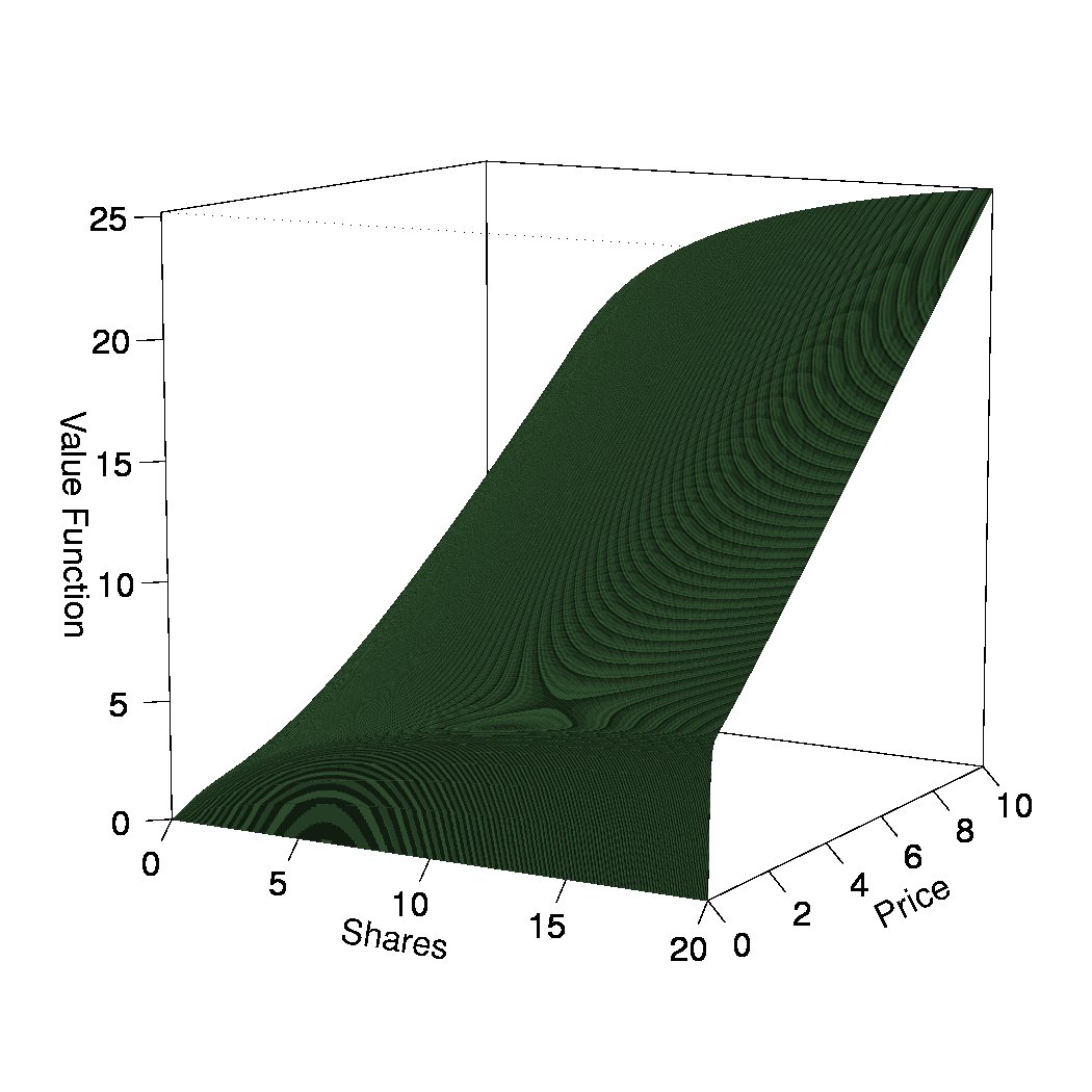
with σ>0\sigma>0. In this case the value function is always finite, regardless of μ\mu, due to the exponential decay of the discount factor. Since 0 is an absorbing boundary for this process the boundary conditions are given by (2.17). Figure 2(a) shows the value function obtained by the scheme.
Refer to caption
(a) Value function in the BM case with parameters λ=0.5\lambda=0.5, μ=4\mu=4, σ=0.5\sigma=0.5 and β=1\beta=1.
Refer to caption
(b) Continuation-trade region in the BM case. The solid line shows the contour with parameters λ=0.5\lambda=0.5, μ=4\mu=4, σ=0.5\sigma=0.5 and β=1\beta=1. In the other lines only the indicated parameter has been changed.
Figure 2: Value function and continuation-trade region in the BM case.

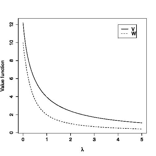
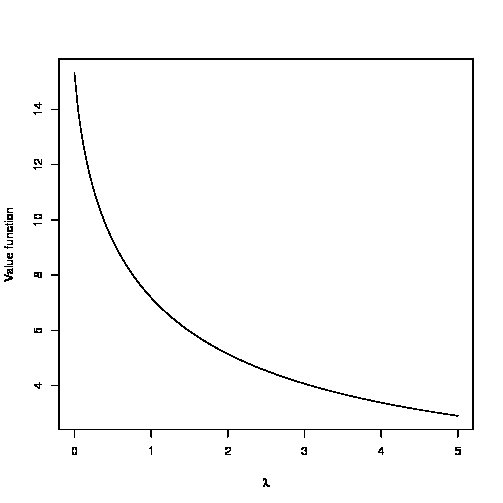
First note that the conditions of Theorem 3.3 are not satisfied, that is U⁡(x,p)≠x​pU(x,p)\neq xp, and therefore 𝒯≠𝒪\mathcal{T}\neq\mathcal{O}, as shown in figure 2(b). Thus, in this case the optimal strategy would be to trade very fast in the trading region until the state variable hit the free boundary. The figure also shows how the different parameters affect the continuation/trade regions. Now, let’s see how the change in the parameters of the model affect the value function VV. Figure 3(a) shows that the value function is very sensitive to changes in the parameter λ\lambda for small values but not so much for large values. This behavior is common to both processes GBM (described by theorem 3.3) and BM. This means that the bigger the investor (i.e. the larger the price impact) the less sensitive to small changes in the value of λ\lambda. Clearly the value function decreases as the impact increases.

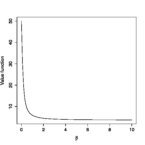
If β=0\beta=0, the value function would not be finite for any μ>0\mu>0, so small values of β\beta yield a very large value of VV. As β\beta increases the effect in VV is diminishing. Also, the investor has to act greedily and therefore the trade region approaches to 𝒪\mathcal{O} and VV approaches to WW.

Refer to caption
(a) Change in V⁡(5,2)V(5,2) as λ\lambda varies and μ=4\mu=4, σ=0.5\sigma=0.5 and β=1\beta=1.
Refer to caption
(b) Change in V⁡(5,2)V(5,2) as β\beta varies and μ=4\mu=4, σ=0.5\sigma=0.5 and λ=0.5\lambda=0.5.
Refer to caption
(c) Change in V⁡(5,2)V(5,2) as μ\mu varies and λ=0.5\lambda=0.5, σ=0.5\sigma=0.5 and β=1\beta=1.
Refer to caption
(d) Change in V⁡(5,2)V(5,2) as σ\sigma varies and μ=4\mu=4, λ=0.5\lambda=0.5 and β=1\beta=1.
Figure 3: Change in the parameters of the model BM.

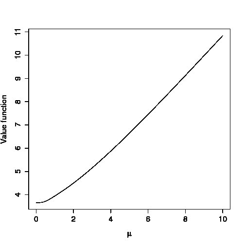
For μ≤0\mu\leq 0 it is not optimal to wait at all, so V=WV=W, but as μ\mu increases clearly the value function increases in an almost linear fashion.

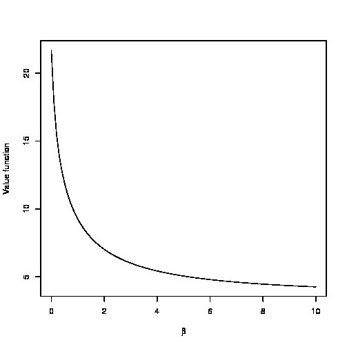
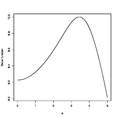
The effect of σ\sigma in the value function is probably the most interesting one. In figure 3(d) we see that it is beneficial for the investor to have some variance in the asset but not too much. An explanation for this is that when the variance increases it is more likely for the price process to enter the trading region. On the other hand, if the variance is too big, the process can hit 0 too fast. Clearly the variance of the revenue increases with σ\sigma, thus as part of future research it would be interesting to consider the risk aversion of the investor.
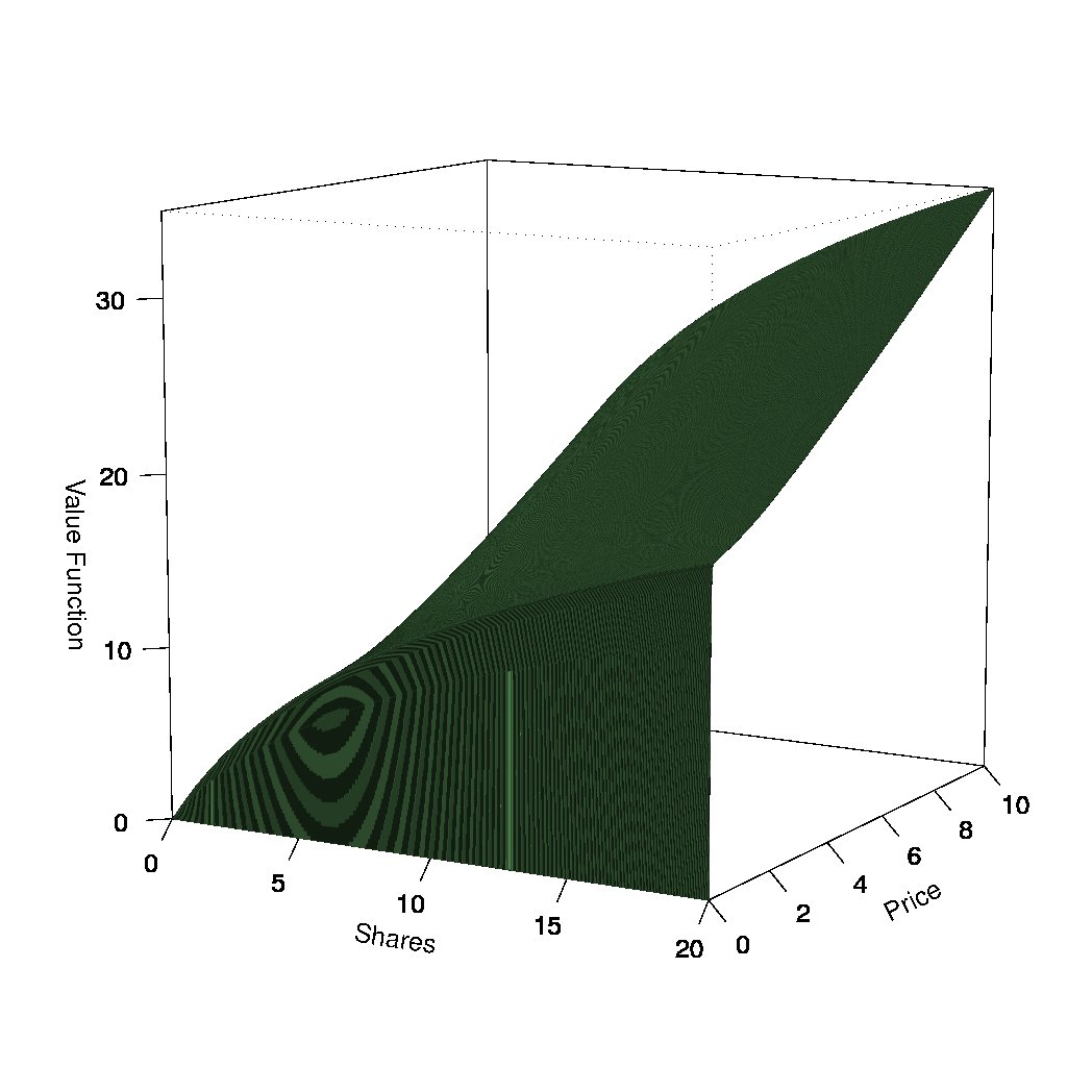
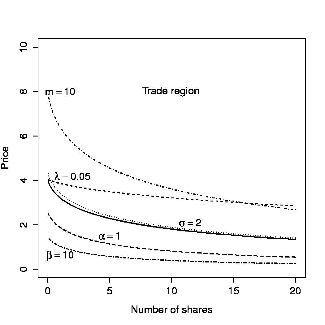
Refer to caption
(a) Value function in the OU case with parameters λ=0.5\lambda=0.5, α=4\alpha=4, σ=0.5\sigma=0.5, m=5m=5 and β=1\beta=1.
Refer to caption
(b) Continuation-trade region in the OU case. The solid line shows the contour with parameters λ=0.5\lambda=0.5, α=4\alpha=4, σ=0.5\sigma=0.5, m=5m=5 and β=1\beta=1. In the other lines only the indicated parameter has been changed.
Figure 4: Value function and continuation-trade region in the mean-reverting case.

The second example is when the price follows the Ornstein–Uhlenbeck process. Then the price process becomes

d​Pt=α⁡(m−Pt)​d​t+σ​d​Bt−λ​Pt​d​ξt,dP_{t}=\alpha(m-P_{t})dt+\sigma dB_{t}-\lambda P_{t}d\xi_{t},

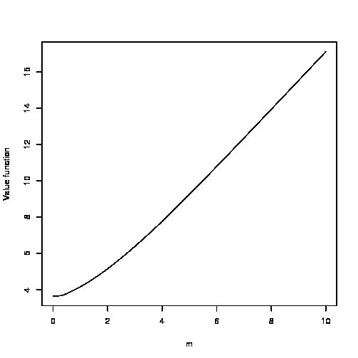
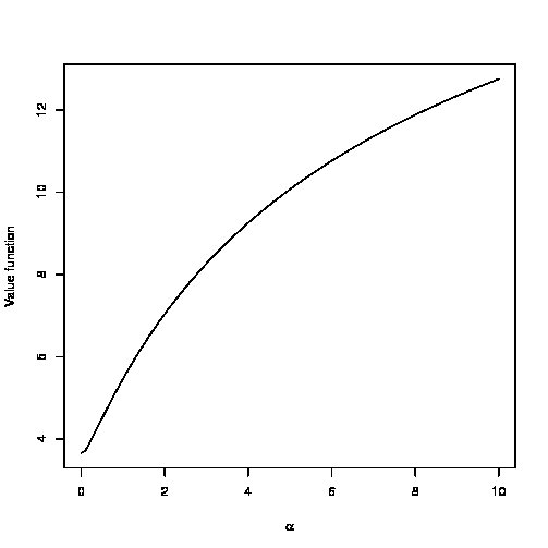
with σ,α>0\sigma,\alpha>0. As in the case of arithmetic Brownian motion, the boundary conditions are given by (2.17), since 0 is an absorbing boundary for this process. Figure 4 shows the value function and the continuation-trade region. Again, this case does not fit within Theorem 3.3, so the strategy is similar to the BM case. Also, the sensitivity of the function to the parameters is similar to the previous case. The only parameter that is exclusive to the mean-reverting process is the resilience factor α\alpha. As we increase α\alpha the value function increases (Figure 5(d)) and the continuation region grows (Figure 4(b)).
Refer to caption
(a) Change in V⁡(5,2)V(5,2) as λ\lambda varies and m=5m=5, σ=0.5\sigma=0.5, α=4\alpha=4 and β=1\beta=1.
Refer to caption
(b) Change in V⁡(5,2)V(5,2) as β\beta varies and m=5m=5, σ=0.5\sigma=0.5, α=4\alpha=4 and λ=0.5\lambda=0.5.
Refer to caption
(c) Change in V⁡(5,2)V(5,2) as mm varies and α=4\alpha=4, σ=0.5\sigma=0.5, β=1\beta=1 and λ=0.5\lambda=0.5.
Refer to caption
(d) Change in V⁡(5,2)V(5,2) as α\alpha varies and λ=0.5\lambda=0.5, σ=0.5\sigma=0.5, m=5m=5 and β=1\beta=1.
Refer to caption
(e) Change in V⁡(5,2)V(5,2) as σ\sigma varies and α=4\alpha=4, λ=0.5\lambda=0.5, m=5m=5 and β=1\beta=1.
Figure 5: Change in the parameters of the model OU.

6 Conclusions

The main goal of this work was to characterize the value function of the optimal execution strategy in the presence of price impact and fixed transaction cost over an infinite horizon. We formulated the problem using two different stochastic control settings. In the impulse control formulation we showed that the value function is the unique continuous viscosity solution of the Hamilton-Jacobi-Bellman equation associated to the problem whenever the transaction cost is strictly positive. The second formulation ruled out any transaction cost and admitted continuous singular controls only. In this case we also proved continuity and uniqueness of the value function under the viscosity framework. The next step, part of future research, would be to find the regularity of the value function. Numerical results provided in this paper, at least for the second formulation, suggest that the function is more than just continuous and that its regularity is related with the regularity of the function UU defined in Section 2. Although any impulse control is a singular control, in general the expected revenue obtained when applying the same impulse control in both formulation is different. However, the value function may be the same. In fact, we were able to show that this is the case for a special type of price impact and provide the explicit solution. The question if this is true in general is still unanswered. This is particularly challenging since the subsolution property for the HJB equation (2.9), when there is no transaction cost, has no information at all. Try to find answers is part of future work. Another important conclusion is that the HJB equation for the regular control formulation, () has not enough information to characterize the solution. From an economic viewpoint, it would be important to study the effect of the price impact in hedging strategies and how they are different to the strategies obtained in classical models, e.g. Delta-hedging in Black-Scholes setting. Include utility functions to account for risk aversion is another important extension of this work. Finally, the finite time horizon natural extension is currently in preparation.

Appendix A Proof of (ℳ​V)∗≤ℳ​V∗(\mathcal{M}V)^{*}\leq\mathcal{M}V^{*}

Let φ\varphi be a locally bounded function on 𝒪¯\bar{\mathcal{O}}. Let (yn)(y_{n}) be a sequence in 𝒪\mathcal{O} such that (yn)→y0(y_{n})\rightarrow y_{0} and

limn→∞ℳ​φ​(yn)=(ℳ​φ)∗​(y0).\lim_{n\rightarrow\infty}\mathcal{M}\varphi(y_{n})=(\mathcal{M}\varphi)^{*}(y_{0}).

Since φ∗\varphi^{*} is usc and Γ\Gamma is continuous, for each n≥1n\geq 1 there exists 0≤ζn≤xn0\leq\zeta_{n}\leq x_{n} such that

ℳ​φ∗​(yn)=φ∗​(Γ⁡(yn,ζn))+ζn​α​(ζn,pn)−k.\mathcal{M}\varphi^{*}(y_{n})=\varphi^{*}(\Gamma(y_{n},\zeta_{n}))+\zeta_{n}\alpha(\zeta_{n},p_{n})-k.

The sequence (ζn)(\zeta_{n}) is bounded (since xn→x0x_{n}\rightarrow x_{0}) and therefore converges along a subsequence to ζ∈[0,x0]\zeta\in[0,x_{0}]. Hence

(ℳ​φ)∗​(y0)\displaystyle(\mathcal{M}\varphi)^{*}(y_{0}) =limn→∞ℳ​φ​(yn)\displaystyle=\lim_{n\rightarrow\infty}\mathcal{M}\varphi(y_{n})
≤lim supn→∞ℳ​φ∗​(yn)\displaystyle\leq\limsup_{n\rightarrow\infty}\mathcal{M}\varphi^{*}(y_{n})
=lim supn→∞φ∗​(Γ⁡(yn,ζn))+ζn​α​(ζn,pn)−k\displaystyle=\limsup_{n\rightarrow\infty}\varphi^{*}(\Gamma(y_{n},\zeta_{n}))+\zeta_{n}\alpha(\zeta_{n},p_{n})-k
≤φ∗​(Γ⁡(y0,ζ))+ζ​α​(ζ,p0)−k\displaystyle\leq\varphi^{*}(\Gamma(y_{0},\zeta))+\zeta\alpha(\zeta,p_{0})-k
≤ℳ​φ∗​(y0).\displaystyle\leq\mathcal{M}\varphi^{*}(y_{0}).

References

  • Almgren (2003) R. Almgren. Optimal execution with nonlinear impact functions and trading-enhanced risk. Applied Mathematical Finance, 10(1):1–18, January 2003.
  • Almgren and Chriss (2000) R. Almgren and N. Chriss. Optimal execution of portfolio transactions. Journal of Risk, 3:5–39, 2000.
  • Bank and Baum (2004) P. Bank and D. Baum. Hedging and portfolio optimization in financial markets with a large trader. Math. Finance, 14(1):1–18, 2004.
  • Bertsimas and Lo (1998) D. Bertsimas and A. W. Lo. Optimal control of execution costs. Journal of Financial Markets, 1(1):1–50, April 1998.
  • Çetin et al. (2004) U. Çetin, R. Jarrow, and P. Protter. Liquidity risk and arbitrage pricing theory. Finance Stoch., 8(3):311–341, 2004.
  • Chan and Lakonishok (1995) L.K.C. Chan and J. Lakonishok. The behavior of stock prices around institutional trades. Journal of Finance, 50(4), September 1995.
  • Crandall et al. (1992) M. G. Crandall, H. Ishii, and P. L. Lions. User’s guide to viscosity solutions of second order partial differential equations. Bulletin of the American Mathematical Society, 27(12):1–67, July 1992.
  • Cvitanić and Ma (1996) J. Cvitanić and J. Ma. Hedging options for a large investor and forward-backward SDE’s. Ann. Appl. Probab., 6(2):370–398, 1996.
  • Davis and Norman (1990) M.H.A. Davis and A.R. Norman. Portfolio selection with transaction costs. Math. Oper. Res., 15(4):676–713, 1990.
  • Dayanik and Karatzas (2003) S. Dayanik and I. Karatzas. On the optimal stopping problem for one-dimensional diffusions. Stochastic Processes and their Applications, 107(2):173–212, October 2003.
  • Fleming and Soner (2006) W.H. Fleming and H.M. Soner. Controlled Markov Processes and Viscosity Solutions. Springer, second edition, 2006.
  • Frey (1998) R. Frey. Perfect option hedging for a large trader. Finance and Stochastics, 2(2):115–141, 1998.
  • He and Mamaysky (2005) H. He and H. Mamaysky. Dynamic trading policies with price impact. Journal of Economic Dynamics and Control, 29(5):891–930, 2005.
  • Holthausen et al. (1990) R.W. Holthausen, R. Leftwich, and D. Mayers. Large-block transactions, the speed of response, and temporary and permanent stock-price effects. Journal of Financial Economics, 26(1):71–95, July 1990.
  • Ishii and Lions (1990) H. Ishii and P. L. Lions. Viscosity solutions of fully nonlinear second-order elliptic partial differential equations. Journal of Differential Equations, 83(1):26 – 78, 1990.
  • Ishii (1993) K. Ishii. Viscosity solutions of nonlinear second order elliptic pdes associated with impulse control problems. Funkcialaj Ekvacioj, 36:123–141, 1993.
  • Ishikawa (2004) Y. Ishikawa. Optimal control problem associated with jump processes. Applied Mathematics and Optimization, 50(1):21–65, 2004.
  • Korn (1998) R. Korn. Portfolio optimisation with strictly positive transaction costs and impulse control. Finance and Stochastics, 2(2):85–114, 1998.
  • Kushner and Dupuis (1992) H. Kushner and P. Dupuis. Numerical methods for stochastic control problems in continuous time. Springer-Verlag, New York, 1992.
  • Ly Vath et al. (2007) V. Ly Vath, M. Mnif, and H. Pham. A model of optimal portfolio selection under liquidity risk and price impact. Finance Stoch., 11(1):51–90, 2007.
  • Ma and Yong (1999) Jin Ma and Jiongmin Yong. Dynamic programming for multidimensional stochastic control problems. Acta Mathematica Sinica, 15:485–506, 1999. ISSN 1439-8516.
  • Øksendal and Reikvam (1998) B. Øksendal and K. Reikvam. Viscosity solutions of optimal stopping problems. Stochastics An International Journal of Probability and Stochastic Processes: formerly Stochastics and Stochastics Reports, 62(3):285– 301, 1998.
  • Øksendal and Sulem (2002) B. Øksendal and A. Sulem. Optimal consumption and portfolio with both fixed and proportional transaction costs. SIAM Journal on Control and Optimization, 40(6):1765–1790, 2002.
  • Øksendal and Sulem (2005) B. Øksendal and A. Sulem. Applied Stochastic Control of Jump Diffusions. Springer, 2005.
  • Protter (2004) P. Protter. Stochastic Integration and Differential Equations. Springer-Verlag, Berlin, second edition, 2004.
  • Schied and Schöneborn (2009) A. Schied and T. Schöneborn. Risk aversion and the dynamics of optimal liquidation strategies in illiquid markets. Finance Stoch., 13(2):181–204, 2009.
  • Schied et al. (2010) A. Schied, T. Schöneborn, and M. Tehranchi. Optimal Basket Liquidation for CARA Investors is Deterministic. Applied Mathematical Finance, 17:471–489, 2010.
  • Subramanian and Jarrow (2001) A. Subramanian and R. Jarrow. The liquidity discount. Mathematical Finance, 11(4):447–474, 2001.