UMD-PP-10-010 Higgs Production from Gluon Fusion in Warped Extra Dimensions
Abstract
We present an analysis of the loop-induced couplings of the Higgs boson to the massless gauge fields (gluons and photons) in the warped extra dimension models where all Standard Model fields propagate in the bulk. We show that in such models corrections to the and couplings are potentially very large. These corrections can lead to generically sizable deviations in the production and decay rates of the Higgs boson, even when the new physics states lie beyond the direct reach of the LHC.
I Introduction
Warped extra dimensions, à la Randall-Sundrum model (RS) present one of the most elegant solutions to the Standard Model (SM) hierarchy problem [1]. Placing SM fields in the bulk of the extra dimension can simultaneously explain the hierarchies of the SM fermion masses [2, 3, 4]. Such models provide a very attractive way to suppress flavor violation by the so called RS Glashow-Iliopoulos-Maiani(GIM) mechanism [2, 5, 6]. The electroweak precision tests put important bounds on the scale of new physics, but by introducing custodial symmetries [7, 8] one can have it around few TeV [7, 9, 8].
In this paper, we will analyze the Higgs couplings to massless vector bosons in RS models where all SM fields are in the bulk, and the modification to the and couplings arises from integrating out Kaluza-Klein (KK) partners of the SM fields. Previous works on this topic for RS models have been done in [10, 11, 13, 12, 14]11 1 One of the main differences between our work and previous analysis is that we present analytical results for the contribution of the full KK fermion tower. Other subtle differences are discussed in the main text.. These effects were also studied in models of warped extra dimensions in which the Higgs arises as Pseudo-Nambu-Goldstone boson (PNGB) [15] and within the effective theory formalism [16, 17]. The studies of the Higgs production in flat extra dimensions in the models with gauge Higgs unification were carried out in [18]. We will stick to the models with flavor anarchy [5, 6] in which the hierarchies in masses and mixings in the the fermion sector are explained by small overlap integrals between fermion wave functions and the Higgs wave function along the extra dimension. Previous studies of this framework have mainly focused on bounds on the KK scale coming from new flavor violating sources. In spite of the RS-GIM mechanism, it was still found that processes mediated by the KK gluon push the mass of the KK excitations to be above TeV [19, 20, 21], making them very hard to produce and observe at the LHC [22]. These bounds coming from flavor violation in low energy observables can be relaxed by introducing additional flavor symmetries [20, 24, 23, 25], or by promoting the Higgs to be a 5D bulk field (instead of being brane localized) [26, 27]. A similar tension was found in the lepton sector in [28], making scale of TeV still compatible with experiments. Lower KK scales can be achieved by changing the fermion representations [29] or by introducing flavor symmetries [24]. It is interesting to point out that flavor violating effects can also be mediated by the radion [30], a graviscalar degree of freedom which might be generically the lightest new physics state and therefore may lead to important phenomenological bounds. More recently, it has also been pointed out that models with fermions in the bulk give rise to flavor violation in the couplings of Higgs to SM fermions [31, 32], leading to interesting constraints from processes and to flavor violating collider signatures such as (see also the most recent analysis of [33, 12] for further details). Other interesting collider effects like rare top decays were discussed in [34].
The outline of the paper is as follows: in section II, we consider the effect of just two vector-like heavy fermions, one singlet under and one doublet. This simple case helps us understand in simple terms the effects caused by the full tower of KK fermions in a realistic 5D setup. In section III we present a calculation of the and couplings for the simple model where all the fermions are in a doublet representation of or . In this section and in Appendix A we also present a simple way to evaluate the complete KK fermion tower contribution to and couplings. Having explained and derived the new contributions to the Higgs couplings caused by the heavy KK fermions, we proceed in section IV to study quantitatively the main phenomenological effects and outline our conclusions in section V.
II Warm-up: New Vector-Like Fermions
We begin by computing the new contribution to the coupling using effective theory with just the zero and first KK modes, where we only consider one family of light quarks (say, up and down quarks) augmented by the presence of two heavy vector-like fermions, one in doublet representation of and the other in singlet representation. This effective theory description has the advantage of being economical and gives lucid physical intuition of the source of new physics contribution. Therefore, we adopt this approach in this section just to illustrate the essential points of our calculation. Moreover, the calculation is more general is the sense that it applies to any Beyond Standard Model (BSM) model in which there exist extra vector-like fermions which mix with SM fermions (see [35] for a similar discussion). The full calculation of the coupling in the 5D warped extra dimension model will be carried out in the next section.
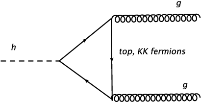
To start, we review here the Higgs boson production through gluon fusion in SM. The coupling between gluon and Higgs mainly comes from top quark loop (See Fig. 1). The partonic cross section for is [36]
| (1) |
where the sum is for all SM fermions, is invariant mass squared of the two incoming gluons, , and are Yukawa couplings and masses of the quarks, and the form factor for fermion in the loop is
| (2) |
where
| (3) |
We note that for i.e. , the form factor tends to be unity, while for i.e. , the form factor tends to zero. For reference, we consider a Higgs boson with mass GeV, then for c-quark, we have ; and for a KK fermion with mass GeV, we have . Therefore, it is a good approximation to treat the form factors for KK fermions as unity, while for light quarks, we can safely ignore their contributions.
In the effective theory with just one KK mode, we have zero mode fermions () and first KK fermions (), where denote the up-type quark from doublet, and denote the up-type quark from singlet. Then we have the following mass matrix:
where etc. are the Yukawa couplings between the corresponding chiral fermions, and is the Higgs VEV (note that it is not the same as ). The Yukawa couplings matrix is given by
To calculate these fermion contributions to the coupling, we assume that the masses of the KK fermions , and therefore their form factors are approximately unity. Before proceeding let us classify different effects contributing to the shift of coupling from that of the SM:
- •
relation between mass and Yukawa coupling of the lightest state (SM fermion) is modified from the SM value ;
- •
we have loop of KK fermion running in the triangle diagrams (see Fig. 1).
So we should calculate
| (18) |
where and are the fermion mass and Yukawa matrices given in Eq. (II) and (II)22 2 Note that the real part of the Yukawa coupling will lead to the operator , and the imaginary part will lead to the operator . For simplicity in this paper we everywhere will assume that we have only operator.. The first term on the LHS of the above equation gives the contribution from the SM fermion (lightest mass eigenstate), and the second term comes from the contributions of heavy KK fermions. Note that , therefore, we can use the following trick to calculate the trace [37]:
| (19) |
we also have
| (20) |
Now we expand to first order in :
| (21) |
Note that the masses and Yukawa couplings of the SM fermions are also modified (see [32] for details),
| (22) |
where the last expression was derived using the following assumption (). This assumption is true the quarks of the first two generations, and the extra contribution which is important for the quarks of the third generation will be presented in the next section. Now Eq. (18) reduces to
| (23) |
We can see that for the light generation quarks, , we get , which is just the contribution coming from the KK modes. Note that this contribution is proportional to , which is the product of Yukawa couplings of the KK fermions of opposite chiralities, this structure of the contribution will become essential in calculating the effects in realistic warped model in the next section. It is interesting to see that even though the light SM quarks give negligible contribution to coupling, their KK partners can give sizable new contributions. In addition, there would be an multiplicity enhancement of these KK contributions due to the number of flavors.
The analysis above showed that additional vector-like fermions which mix with SM fermions can alter the coupling significantly. In warped extra dimension models with 5D fermions propagating in the bulk, these extra vector-like fermions naturally come up as the KK towers of fermions. Therefore, we expect generically sizable new physics contributions to coupling in this class of models. We carry out the detailed calculations in warped extra dimension in the next section.
III Minimal Warped Extra Dimension Model with Custodial Protection
In this section, we first calculate the KK fermion contributions to coupling in warped extra dimensions (RS). We then apply similar techniques to calculate both KK fermion and KK gauge boson contributions to coupling. We show that simple analytical formulas can be obtained for these new physics contributions.
III.1 coupling in RS
In this subsection, we consider the effect of the full KK fermion tower on coupling. We consider models with bulk gauge group , which is motivated to ease the bound from electroweak precision test [7]. We consider here just a single family of quarks for the sake of simplicity. A generalization to 3 generation quarks can be easily applied later. For the quark fields, we consider the simple spinorial representation with the following field contents:
The first multiplet is a doublet of and the last two are doublets of . The boundary conditions are denoted for the corresponding chirality. They have the following Yukawa couplings 33 3 We consider here a general bulk Higgs [38] with vector-like Yukawa coupling for simplicity.
| (31) |
Note that , are dimensionless and order one, and is the curvature scale. After KK decomposition in the basis where Higgs vev is zero, we have zero modes and the KK modes . For up-type quarks, we have the following infinite dimensional mass matrix
where are KK indices. The Yukawa couplings matrices are defined e.g. by
| (41) |
i.e. it is an integral of product of Higgs and fermion wavefunctions, where is a profile of the Higgs field normalized in the following way
| (42) |
The KK mass matrices are diagonal, e.g. . One naively might think that the couplings vanish in the limit of brane Higgs due to the odd boundary conditions of and , so it is safe to ignore them in this matrix. But these are precisely the odd operators described in detail in [32] (detailed analysis without these operators was presented in [13]). These operators as was shown in [32] lead to flavor violation in the Higgs sector, and they are also essential in evaluating the coupling44 4 These operators can be mimicked by higher dimensional derivative operators [32], which shows UV sensitivity of the effect.. To avoid subtleties with wave function being discontinuous at IR brane we will assume that the Higgs is 5D bulk field and only at the end we will take a brane Higgs limit.
Now we can use the same determinant trick, the determinant of the mass matrix to the order of is
| (43) |
Now we get
| (44) |
Again, for the light generation quarks there are corrections to the SM fermion masses and Yukawa couplings [32]
| (45) | |||||
| (46) | |||||
Therefore
| (47) |
So the total contribution to coupling by light generation quarks and their KK partners is (see Eq. 18)
| (48) |
Note that this result is very similar to the one we obtained in the last section (Eq. 23), except for an extra term corresponding to the contribution of extra states in the doublet representation of . For light generations, the last term is negligible, and we are left with first two terms. The first two terms can be written as
| (49) | |||
Now we have to evaluate the following sums
| (50) |
We can calculate them by using equations of motion for fermion wavefunctions (see discussion in the Appendix A). From the forms of these sums (see Eq. (69)), we see that we need to evaluate the integrals of Higgs wavefunction times and . This can be done for general bulk Higgs. But for illustration purpose we take the brane Higgs limit of bulk Higgs. Then we get
| (51) |
and Eq. (49) now reduces to
| (52) |
Therefore, for light generations, the contribution to coupling is , which comes just from KK fermions and is independent of fermion bulk mass parameters.
For the third generation quarks there will be an extra contribution to the formula in (Eq. 47) which we parameterize following [32] as (see Appendix C for details). This gives us additional contribution relative to (Eq. 48)
| (53) |
Also in this case contributions of the SM bottom and top qaurks are no longer negligible, so we have to include them
| (54) |
Note that now Yukawa couplings of the top and bottom quarks are shifted( see discussion in Appendix C).
It is simple to generalize the above result to three generations. The KK towers of the quarks give a contribution proportional to , and we have to combine them with the effect coming from top and bottom quarks. To summarize, compared with SM, the Higgs production cross-section from gluon fusion in RS is
| (55) |
where and , with , the shifted top and bottom Yukawa couplings in RS (reference [12] presented numerical results for the analysis of the brane Higgs model including odd operators, however, it is hard to compare it with our result due to different particle content of the models). We consider here the ratio in order to reduce the uncertainty coming from higher order QCD corrections. It is also important to notice that in the case when the couplings of the and are not equal the ratio might be quite significant, see discussion and analysis in [13]. In the rest of the paper we will assume that and custodial have the same gauge couplings (see appendix B for discussion of VEV shift in this case).
It is also interesting to point out that the same diagrams that contribute to the gluon fusion will also contribute to the modification of the di-Higgs production. This might become an interesting option to disentangle new physics contribution (see discussion in the effective field theory approach in [35]).
III.2 coupling in RS
The calculation of the coupling comes from similar diagrams as the one for the coupling, the only difference now is that we have to take into account contributions of the towers of charged KK gauge bosons and KK leptons. We will again use the simplest custodial model where leptons are in the doublet representation of or . We can calculate their contribution in the same way as we did for the quarks. Contribution of the KK tower of the was presented in [13], so here we just quote their results and the reader can find more details about the derivation in the Appendix B. The contribution of the tower of the KK is given by
| (56) |
where is coupling between Higgs field and the n-th KK modes (mass eigenstates) of the , and is coupling between SM and the Higgs. is the form-factor for the gauge bosons (see Eq. (76)). Including the modification of the coupling between SM and Higgs, this sum can be expresssed in the following way:
| (57) | |||||
where and are the 5D gauge couplings of and respectively. Adding both fermion and gauge boson contributions together, now we can present our results for the ratio of between RS and SM:
| (58) |
IV Phenomenology
In this section, we discuss the phenomenology of the Higgs boson in warped extra dimensions. We focus our study on the Higgs production through gluon fusion and the branching fraction of decay. We will compare our results with that of holographic PNGB Higgs model studied in [15].
To get a handle on the size of new physics contributions, we scan the parameter space of RS with the assumption of flavor anarchy, i.e. the 5D Yukawa matrices are order one and uncorrelated. We find the set of 5D Yukawa couplings and fermion zero mode wavefunctions which give the correct SM quark masses and CKM mixing. We then calculate and using Eq. (55) and (58), and find the ratio with that of SM. The result of the scan for bulk Higgs is shown in Fig. 2.
We can see from the plot in Fig. 2 that the new physics contribution to tends to be positive and gets larger for lower KK scale. Also the new physics contribution to and are correlated: an increase in is accompanied by a decrease in .

Before proceeding further let us stop and see whether we can understand these results intuitively. First let us focus on the enhancement of the Higgs production due to gluon fusion. As we argued in the sections III.1 these effects come mainly from the modification of the top Yukawa coupling and from the loop with KK fermions. As was shown in [32] top Yukawa coupling is reduced compared to the SM value, so naively one should expect the reduction of the Higgs production. But let us now look on the contribution of the KK modes. One can see from (Eq. 55) that this contribution is proportional to which is always positive, so the sign of this contribution is fixed. Also the typical size of this term will be roughly equal to where N is number of SM families and is an average size of the Yukawa couplings, so adding both up and down quark KK towers will lead to an overall enhancement factor of 18.66 6 One can see that for sufficiently large Yukawa couplings our expansion in powers of might become ill defined, and also contribution of the higher order loops with KK fermions and Higgs might become important, so the one loop result becomes not reliable if the new physics contribution is much larger than that of the SM. At the same time we would like to note that our result even for the large 5D Yukawa couplings will give a typical size of the expected correction to the SM coupling. Therefore KK fermions give a large positive contribution to . Reduction of the can be understood from the fact that in the SM the dominant contribution comes from the loop with , and the fermion contribution has an opposite sign, thus enhancement of the fermion contributions effectively decreases the overall coupling.
This implication is two-fold. First, it means that even with a KK scale out of the reach of the LHC ( TeV), we can still probe the framework of warped extra dimension by precision measurements of various Higgs production and decay processes. Second, by comparing our result with that of [15], we can see that can be used to distinguish between RS with bulk Higgs and holographic PNGB Higgs model (or gauge-Higgs unification). In the latter model, a reduction is usually expected, which can be contrasted with our results for bulk Higgs. Note that the difference in these two models comes from the extra symmetry in PNGB Higgs, which constrains the Higgs interactions (see discussion in [16, 17]).
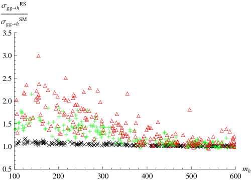
To study the dependence of new physics contributions on the Higgs boson mass, we plot in Fig. 3 the ratio vs. for various KK scales. We can see that the new physics contribution decreases as increase from to GeV. This can be understood from the fact that in SM, the form factor for the top quark attains its largest value when . Since in RS with bulk Higgs, the top quark Yukawa coupling is reduced compared to that of SM, there is a larger negative new physics contribution to coupling when , leading to a smaller total new physics contribution.
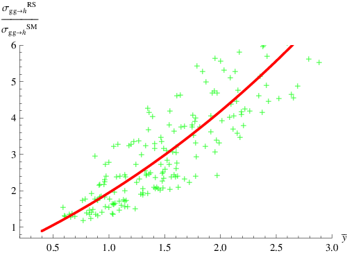
In Fig. 4, we plot the dependence of the ratio on the average size of the 5D Yukawa couplings. We can see quite clearly that the size of new physics contribution increases as the 5D Yukawa couplings increases. This is expected from the fact that KK fermion contributions are proportional to . In the framework of flavor anarchy, the 5D Yukawa couplings are order one. We can see from Fig. 4 that for order one Yukawa couplings, we have sizable new physics contributions to .
So far we have been assuming that the Higgs is the bulk field and 5D Yukawa couplings are vector-like i.e.
| (59) |
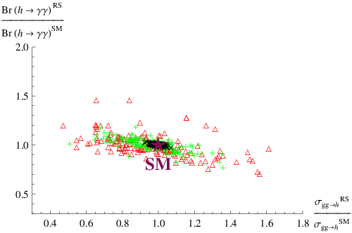
In the case where the Higgs is a 5D bulk field this condition of is forced by the 5D Lorentz symmetry. But the Higgs can be brane localized or even a bulk Higgs might have brane localized couplings and these couplings do not have to respect 5D bulk Lorentz symmetry. So generally speaking , and they could be independent of each other. Let us see how this might modify our results. The first thing to notice is that the contribution of the tower of KK modes now has the following structure . Before proceeding further we immediately see that the overall sign of the contribution is not fixed any more! So we cannot predict in generic RS model the sign of the effect: whether it is enhancement or suppression for both and couplings. This is shown in Fig. 5. We can see that the size of new physics contribution is generically large for moderate KK scale, but now its sign can be both positive and negative.
V Conclusions
In conclusion, we summarize the results presented in the paper. We calculated the corrections to the and couplings in RS at one loop order. We have found that the new physics states can modify significantly these couplings. We have shown that the dominant contribution to these coupling comes from the towers of KK fermions running inside triangle diagrams. We have shown that the KK towers of the light fermions do contribute significantly to these couplings, contrary to the models with Higgs being a PNGB boson where this contribution is sub-leading. We have shown that in the models with the Higgs in the bulk and Yukawa couplings being vectorlike (), coupling becomes enhanced and coupling suppressed compared to that of SM, even though the top Yukawa coupling is suppressed compared to the SM value. This naively counterintuitive result is explained by the fact that the contribution of the KK towers of all SM fermions is so strong that it overcomes the effect from suppression of the top Yukawa coupling. Modification of the Higgs production cross-section remains significant even for a KK scale far from LHC accessibility. Specifically, we can get order one corrections even with lightest KK modes above 5 TeV. For the generic models with Higgs on the brane or bulk Higgs with brane Yukawa couplings the sign of the effect remains unpredictable. We might have enhancement as well as suppression, but the parametric size of the effect remains the same. The total effect comes from collective contributions of the KK partners of all generations. Therefore, the size of these new physics contributions is large, even if the KK fermions are heavy. This shows us that in the absence of new resonances an analysis of the Higgs couplings might become a very important tool in understanding the structure of BSM physics.
Acknowledgements
We would like to thank Kaustubh Agashe for his encouragement, comments and suggestions. We would also like to thank Matthias Neubert for useful discussion and Uli Haisch, Florian Goertz, Sandro Casagrande and Torsten Pfoh for comments. A.A. and L.Z. would like to thank Maryland Center for Fundamental Physics for support during the completion of this project.
References
- [1] L. Randall and R. Sundrum, Phys. Rev. Lett. 83, 3370 (1999); [arXiv:hep-ph/9905221]; L. Randall and R. Sundrum, Phys. Rev. Lett. 83, 4690 (1999). [arXiv:hep-th/9906064].
- [2] T. Gherghetta and A. Pomarol, Nucl. Phys. B 586, 141 (2000); [arXiv:hep-ph/0003129].
- [3] Y. Grossman and M. Neubert, Phys. Lett. B 474, 361 (2000); [arXiv:hep-ph/9912408].
- [4] H. Davoudiasl, J. L. Hewett and T. G. Rizzo, Phys. Lett. B 473, 43 (2000) [arXiv:hep-ph/9911262]; A. Pomarol, Phys. Lett. B 486, 153 (2000) [arXiv:hep-ph/9911294]; S. Chang, J. Hisano, H. Nakano, N. Okada and M. Yamaguchi, Phys. Rev. D 62, 084025 (2000) [arXiv:hep-ph/9912498].
- [5] K. Agashe, G. Perez and A. Soni, Phys. Rev. D 71, 016002 (2005), [arXiv:hep-ph/0408134].
- [6] S. J. Huber and Q. Shafi, Phys. Lett. B 498, 256 (2001) [arXiv:hep-ph/0010195]; S. J. Huber, Nucl. Phys. B 666, 269 (2003) [arXiv:hep-ph/0303183].
- [7] K. Agashe, A. Delgado, M. J. May and R. Sundrum, JHEP 0308, 050 (2003). [arXiv:hep-ph/0308036].
- [8] K. Agashe, R. Contino, L. Da Rold and A. Pomarol, Phys. Lett. B 641, 62 (2006) [arXiv:hep-ph/0605341].
- [9] M. Carena, E. Ponton, J. Santiago and C. E. M. Wagner, Nucl. Phys. B 759, 202 (2006) [arXiv:hep-ph/0607106] and M. S. Carena, E. Ponton, J. Santiago and C. E. M. Wagner, Phys. Rev. D 76, 035006 (2007) [arXiv:hep-ph/0701055]; C. Bouchart and G. Moreau, Nucl. Phys. B 810, 66 (2009) [arXiv:0807.4461 [hep-ph]].
- [10] B. Lillie, JHEP 0602, 019 (2006) [arXiv:hep-ph/0505074].
- [11] A. Djouadi and G. Moreau, Phys. Lett. B 660, 67 (2008) [arXiv:0707.3800 [hep-ph]].
- [12] S. Casagrande, F. Goertz, U. Haisch, M. Neubert and T. Pfoh, arXiv:1005.4315 [hep-ph].
- [13] C. Bouchart and G. Moreau, Phys. Rev. D 80, 095022 (2009) [arXiv:0909.4812 [hep-ph]].
- [14] G. Cacciapaglia, A. Deandrea and J. Llodra-Perez, JHEP 0906, 054 (2009) [arXiv:0901.0927 [hep-ph]].
- [15] A. Falkowski, Phys. Rev. D 77, 055018 (2008) [arXiv:0711.0828 [hep-ph]].
- [16] G. F. Giudice, C. Grojean, A. Pomarol and R. Rattazzi, JHEP 0706, 045 (2007) [arXiv:hep-ph/0703164].
- [17] I. Low, R. Rattazzi and A. Vichi, JHEP 1004, 126 (2010) [arXiv:0907.5413 [hep-ph]].
- [18] N. Maru and N. Okada, Phys. Rev. D 77, 055010 (2008) [arXiv:0711.2589 [hep-ph]].
- [19] C. Csaki, A. Falkowski and A. Weiler, JHEP 0809, 008 (2008); [arXiv:0804.1954 [hep-ph]].
- [20] A. L. Fitzpatrick, G. Perez and L. Randall, arXiv:0710.1869 [hep-ph].
- [21] M. Blanke, A. J. Buras, B. Duling, S. Gori and A. Weiler, JHEP 0903, 001 (2009) [arXiv:0809.1073 [hep-ph]]; M. Blanke, A. J. Buras, B. Duling, K. Gemmler and S. Gori, JHEP 0903, 108 (2009) [arXiv:0812.3803 [hep-ph]]; M. E. Albrecht, M. Blanke, A. J. Buras, B. Duling and K. Gemmler, JHEP 0909, 064 (2009) [arXiv:0903.2415 [hep-ph]]; M. Bauer, S. Casagrande, L. Grunder, U. Haisch and M. Neubert, Phys. Rev. D 79, 076001 (2009) [arXiv:0811.3678 [hep-ph]]; M. Bauer, S. Casagrande, U. Haisch and M. Neubert, arXiv:0912.1625v1 [hep-ph].
- [22] K. Agashe, A. Belyaev, T. Krupovnickas, G. Perez and J. Virzi, Phys. Rev. D 77, 015003 (2008) [arXiv:hep-ph/0612015]; B. Lillie, L. Randall and L. T. Wang, JHEP 0709, 074 (2007) [arXiv:hep-ph/0701166]; B. Lillie, J. Shu and T. M. P. Tait, Phys. Rev. D 76, 115016 (2007) [arXiv:0706.3960 [hep-ph]]; A. Djouadi, G. Moreau and R. K. Singh, Nucl. Phys. B 797, 1 (2008) [arXiv:0706.4191 [hep-ph]]; M. Guchait, F. Mahmoudi and K. Sridhar, Phys. Lett. B 666, 347 (2008) [arXiv:0710.2234 [hep-ph]]; U. Baur and L. H. Orr, Phys. Rev. D 76, 094012 (2007) [arXiv:0707.2066 [hep-ph]] and Phys. Rev. D 77, 114001 (2008) [arXiv:0803.1160 [hep-ph]]; M. Carena, A. D. Medina, B. Panes, N. R. Shah and C. E. M. Wagner, Phys. Rev. D 77, 076003 (2008) [arXiv:0712.0095 [hep-ph]]; K. Agashe, A. Azatov, T. Han, Y. Li, Z. G. Si and L. Zhu, arXiv:0911.0059 [hep-ph]; K. Agashe et al., Phys. Rev. D 76, 115015 (2007) [arXiv:0709.0007 [hep-ph]]; K. Agashe, S. Gopalakrishna, T. Han, G-Y. Huang and A. Soni, Phys. Rev. D 80, 075007 (2009) [arXiv:0810.1497 [hep-ph]].
- [23] G. Cacciapaglia, C. Csaki, J. Galloway, G. Marandella, J. Terning and A. Weiler, JHEP 0804, 006 (2008) [arXiv:0709.1714 [hep-ph]]; A. L. Fitzpatrick, L. Randall and G. Perez, Phys. Rev. Lett. 100, 171604 (2008); J. Santiago, JHEP 0812, 046 (2008) [arXiv:0806.1230 [hep-ph]]. C. Csaki, G. Perez, Z. Surujon and A. Weiler, Phys. Rev. D 81, 075025 (2010) [arXiv:0907.0474 [hep-ph]]; M. C. Chen, K. T. Mahanthappa and F. Yu, Phys. Rev. D 81, 036004 (2010) [arXiv:0907.3963 [hep-ph]].
- [24] M. C. Chen and H. B. Yu, Phys. Lett. B 672, 253 (2009) [arXiv:0804.2503 [hep-ph]]; G. Perez and L. Randall, JHEP 0901, 077 (2009) [arXiv:0805.4652 [hep-ph]]; C. Csaki, C. Delaunay, C. Grojean and Y. Grossman, JHEP 0810, 055 (2008) [arXiv:0806.0356 [hep-ph]]; F. del Aguila, A. Carmona and J. Santiago, arXiv:1001.5151 [hep-ph].
- [25] C. Csaki, A. Falkowski and A. Weiler, Phys. Rev. D 80, 016001 (2009) [arXiv:0806.3757 [hep-ph]].
- [26] K. Agashe, A. Azatov and L. Zhu, Phys. Rev. D 79, 056006 (2009) [arXiv:0810.1016 [hep-ph]].
- [27] O. Gedalia, G. Isidori and G. Perez, Phys. Lett. B 682, 200 (2009) [arXiv:0905.3264 [hep-ph]].
- [28] K. Agashe, A. E. Blechman and F. Petriello, Phys. Rev. D 74, 053011 (2006) [arXiv:hep-ph/0606021]; C. Csaki, Y. Grossman, P. Tanedo and Y. Tsai, arXiv:1004.2037 [hep-ph].
- [29] K. Agashe, Phys. Rev. D 80, 115020 (2009) [arXiv:0902.2400 [hep-ph]].
- [30] A. Azatov, M. Toharia and L. Zhu, Phys. Rev. D 80, 031701 (2009) [arXiv:0812.2489 [hep-ph]].
- [31] K. Agashe and R. Contino, Phys. Rev. D 80, 075016 (2009) [arXiv:0906.1542 [hep-ph]].
- [32] A. Azatov, M. Toharia and L. Zhu, Phys. Rev. D 80, 035016 (2009) [arXiv:0906.1990 [hep-ph]].
- [33] B. Duling, arXiv:0912.4208 [hep-ph].
- [34] S. Casagrande, F. Goertz, U. Haisch, M. Neubert and T. Pfoh, JHEP 0810, 094 (2008) [arXiv:0807.4937 [hep-ph]];
- [35] A. Pierce, J. Thaler and L. T. Wang, JHEP 0705, 070 (2007) [arXiv:hep-ph/0609049].
- [36] J. Gunion, H. Haber, G. Kane, S. Dawson ”The Higgs Hunter’s Guide” 2000, Westview Press.
- [37] J. R. Ellis, M. K. Gaillard and D. V. Nanopoulos, Nucl. Phys. B 106, 292 (1976).
- [38] G. Cacciapaglia, C. Csaki, G. Marandella and J. Terning, JHEP 0702, 036 (2007), [arXiv:hep-ph/0611358]; H. Davoudiasl, B. Lillie and T. G. Rizzo, JHEP 0608, 042 (2006), [arXiv:hep-ph/0508279].
- [39] J. Hirn and V. Sanz, Phys. Rev. D 76, 044022 (2007) [arXiv:hep-ph/0702005].
Appendix A KK sum rules
In this section we will present a way of efficiently performing KK sums for the fermions 77 7 Similar tricks were discussed in [39] (such as Eq. (50)). Let us look at the equations of motions for the fermions in the absence of the Higgs vev. In the absence of the Higgs vev we can always choose a basis where 5D bulk masses are diagonal, and so we can ignore all the mixings. Let us concentrate on the KK decomposition of the doublet with boundary conditions . The equations of motion of the KK wavefunctions are
| (60) | |||
| (61) |
We take the first equation and rewrite it as:
| (62) |
We now multiply by and integrate between and :
| (63) |
We now use the completeness relation
| (64) | |||||
| (65) |
Based on (Eq 63) we will get
| (66) |
where we have explicitly extracted the zero mode contribution from the sum. Let us note that
| (67) |
and where we have defined the warp factor .
Now we can finally write:
| (68) | |||||
Similarly we can calculate the sum for the other three possible boundary conditions :
| (69) |
Using these relations we can now perform all the necessary sums to calculate the KK fermion contribution to coupling.
Appendix B Gauge boson couplings and contribution to coupling
In this section just for the sake of the completion we present analysis for the modification of the gauge boson coupling to the Higgs boson, and their contribution to the coupling. We start from the modification of the Higgs vev
| (70) |
where GeV, is five dimensional gauge coupling of the custodial , so
| (71) |
This effect will lead to the overall modification of the SM and coupling by the factor for ().
B.1 Couplings of to Higgs in RS
To calculate modification of the coupling we also have to calculate contribution coming from the boson. From the Lagrangian (see [7])
| (72) |
one can immediately deduce coupling between Higgs and .
| (73) |
B.2 Contribution of the KK tower of to the
In this subsection we derive the contribution of the KK modes to the coupling (we will closely follow discussion presented in [13]). First let us denote by the mass squared matrix of the charged gauge bosons, then the coupling to the Higgs boson will be given by the matrix
rotating back to the basis where mass matrix is diagonal we will get
| (74) |
where is a unitary matrix that diagonalizes . We can parameterize the contribution of the gauge boson KK modes to the coupling in the following way:
| (75) |
where is the form factor for vector bosons in the loop [36] ()
| (76) |
where is given by Eq. (3). For KK gauge bosons , and , so we get
| (77) |
To evaluate we can use the following trick [37]
| (78) |
Let us see how the determinant of the gauge boson mass matrix depends on . For simplicity we assume that the Higgs is localized on the IR brane. We denote by values of the profiles on the IR brane for KK modes of and gauge bosons respectively. Then the mass matrix will look like:
One can see from the structure of the matrix that the determinant is equal to
| (84) |
We have checked that for generic bulk Higgs , one can calculate it using mixed position momentum propagators. So the results presented in this section are approximately independent of the Higgs localization. Now we can proceed to the evaluation of the sum in Eq. (77) and substituting result for the determinant we get
| (85) |
Appendix C Review of Higgs Flavor violation
In this appendix we present general formulas for the misalignment between SM fermion masses and Higgs Yukawa couplings in RS(see for details[32]). We define the following quantity to parameterize the misalignment
| (86) |
where are mass matrix and Yukawa couplings of the SM fermions. Then it can be split into two parts
| (87) |
where is the main contribution for the light generations and becomes important only for the third generation of quarks. Then calculations show that for the up type quarks is equal to
| (88) |
where are bulk mass parameters for the multiplets containing zero modes of the SM right-handed and left-handed up quarks respectively. is a diagonal matrix with elements given by the profiles of the corresponding quarks respectively
| (89) |
One can get these expressions by evaluating the sum (Eq. 45) directly using the rules of (Eq. 69) or by solving for the exact wavefunctions profiles as described in [32]. For the other contribution we will get the following expression
| (90) |
where
Note that subdominant contribution is only important for the third generation, and in the text we denote to be equal to .