MAN/HEP/2010/10
June 2010
The Minimal Scale Invariant Extension of
the Standard Model
Lisa Alexander-Nunneley and Apostolos Pilaftsis
School of Physics and Astronomy, The University of Manchester,
Manchester M13 9PL, United Kingdom
ABSTRACT
We perform a systematic analysis of an extension of the Standard Model that includes a complex singlet scalar field and is scale invariant at the tree level. We call such a model the Minimal Scale Invariant extension of the Standard Model (MSISM). The tree-level scale invariance of the model is explicitly broken by quantum corrections, which can trigger electroweak symmetry breaking and potentially provide a mechanism for solving the gauge hierarchy problem. Even though the scale invariant Standard Model is not a realistic scenario, the addition of a complex singlet scalar field may result in a perturbative and phenomenologically viable theory. We present a complete classification of the flat directions which may occur in the classical scalar potential of the MSISM. After calculating the one-loop effective potential of the MSISM, we investigate a number of representative scenarios and determine their scalar boson mass spectra, as well as their perturbatively allowed parameter space compatible with electroweak precision data. We discuss the phenomenological implications of these scenarios, in particular, whether they realize explicit or spontaneous CP violation, neutrino masses or provide dark matter candidates. In particular, we find a new minimal scale-invariant model of maximal spontaneous CP violation which can stay perturbative up to Planck-mass energy scales, without introducing an unnaturally large hierarchy in the scalar-potential couplings.
PACS numbers: 12.60.Fr, 11.15.Ex, 11.10.Hi, 14.60.St, 14.80.Ec
1 Introduction
The Standard Model (SM) [1] is a renormalizable theory with a minimal particle content which realizes the famous Higgs mechanism [2] to account for the origin of mass of the charged fermions and the and bosons. Despite intense scrutiny, the SM remains resilient to new physics and appears to describe the data collected over the years at the LEP collider, TEVATRON and in a number of low-energy experiments with remarkable success. Nevertheless, the SM predicts the existence of the Higgs boson which is associated with the mechanism of electroweak spontaneous symmetry breaking (EWSSB), but which so far has remained elusive. A natural realization of the EWSSB mechanism requires the presence of a negative mass parameter, , in the Higgs potential. The negative mass parameter is the source of the infamous gauge hierarchy problem, in which quantum corrections lead to quadratically divergent terms proportional to , where is an ultra-violet (UV) cut-off scale. This UV cut-off scale is usually associated with the scale of a possible higher-energy theory in which the SM might be embedded, such as Grand Unified Theory (GUT). In the SM, with no intermediate mass scale or theory between the electroweak (EW) and Planck scale GeV, the cancellation of the divergent terms requires excessive fine-tuning. The avoidance of this fine-tuning problem has been the motivation for many studies beyond the SM, including supersymmetry (SUSY). In SUSY this problem is naturally solved, provided the SUSY-breaking mass scale, , stays close to the EW scale, e.g. TeV.
In this paper we discuss a different and very minimal approach to solving the gauge hierarchy problem. It is remarkable that the SM depends on only one mass parameter , whose absence from the Higgs potential renders the complete tree-level Lagrangian of the SM scale invariant (SI). However, as first discussed by Coleman and E. Weinberg [3] and later by Gildener and S. Weinberg [4], quantum corrections generate logarithmic terms which explicitly break the scale invariance of the theory and can trigger EWSSB. Unfortunately, a perturbative SI version of the SM is not both theoretically and phenomenologically viable. Specifically, a perturbative SI version of the SM cannot accommodate the LEP2 limit on the Higgs-boson mass, [5], given the experimental value of the top-quark mass. On the other hand, the large top-quark Yukawa coupling gives rise to an effective potential which is no longer bounded from below (BFB). To overcome this difficulty, several authors [6, 7, 8, 9, 10] have considered various SI extensions to the SI SM either with real or complex singlet scalar fields.
Evidently, one of the main motivations for a SI theory is the natural removal of the term from the Higgs potential. However, its absence alone does not solve the gauge hierarchy problem as terms can still be generated by quantum corrections in a UV cut-off scheme of regularization. This happens because the UV cut-off scheme introduces counter-terms which explicitly violate the symmetry of classical scale invariance that governs the bare Lagrangian. Following the arguments of [9, 11], one has to therefore adopt a regularization scheme which does not break the classical symmetries of the local classical action, in this case scale invariance. Dimensional regularization (DR) [12] is such a SI scheme within which the vanishing of the term is maintained to all orders in perturbation theory. Consequently, the scheme of DR will be used throughout this paper.
An inherent field-theoretic difficulty of a SI model is the incorporation of gravity which requires the introduction of a dimensionful parameter, the Planck mass , into the theory. The presence of the Planck mass explicitly breaks the classical symmetry of scale invariance, thereby reintroducing the issue of quadratic divergences in the theory. Even though addressing this problem lies beyond the scope of this paper, we note that attempts have been made in the literature to provide SI descriptions of quantum gravity [9, 13, 14].
In this paper we study in detail a minimal SI extension of the SM augmented by a complex singlet scalar field, . We call this model the Minimal Scale Invariant extension of the Standard Model (MSISM). Unlike previous analyses [6, 7, 8, 10, 9], we impose no additional constraints on the theory, such as a U(1) symmetry or some specific discrete symmetry acting on . Hence, the MSISM potential contains all possible interactions allowed by gauge invariance:
where the quartic couplings are all dimensionless constants and is the usual SM Higgs doublet. Note that the imposition of scale invariance forbids the appearance of dimensionful mass parameters or trilinear couplings in the potential 11 1 For recent studies of non-SI models with dimensionful self-couplings and with real or complex scalar singlet extensions see [15, 16]..
The tree-level SI scalar potential can possess a large number of different phenomenologically viable flat directions, which may be classified into three major categories: Type I, Type II and Type III. Flat directions of Type I are characterized by a singlet field with vanishing vacuum expectation value (VEV), whereas in flat directions of Type II both and possess non-zero VEVs. Finally, in flat directions of Type III the SM has a zero VEV, which makes it somehow difficult to naturally realize EWSSB and therefore we do not study them in detail in this paper.
In our analysis of the MSISM effective potential, we follow the perturbative approach introduced by Gildener and S. Weinberg (GW) [4]. With the aid of this approach we can analytically calculate the scalar boson mass spectrum and determine the allowed range of parameter space for which the theory remains perturbative, i.e. the theory has perturbative quartic couplings, and which keep the effective potential BFB. Further constraints on the MSISM are obtained from an analysis of the LEP2 data [17] and the electroweak oblique parameters, , and [18, 19]. Of the electroweak oblique parameters, and (the latter associated with Veltman’s parameter [20]) yield the strongest constraints on the range of the scalar-potential quartic couplings.
An interesting feature of the MSISM is that it can be naturally extended by right-handed neutrinos in a SI way, such that a singlet Majorana mass scale, , can be generated if the complex scalar possesses a VEV [21, 10]. The expected size of is typically of the EW scale. This can give rise to a low-scale seesaw mechanism [22], which in turn can offer a natural explanation for the smallness in mass of the light neutrinos as observed in the low-energy neutrino data. Moreover, unlike the SM, the MSISM can realize both explicit and spontaneous CP violation. Of particular interest is a new minimal model of maximal spontaneous CP violation along a maximally CP-violating flat direction of Type II, which can stay perturbative up to energy scales of order , without the need to introduce a large hierarchy among the scalar-potential quartic couplings or between the VEVs of the and fields [23]. The new CP-violating phase could act as a source for creating the observed Baryon Asymmetry in the Universe (BAU), e.g. via a strong first-order electroweak phase transition. Finally, the MSISM can predict stable scalar states that could qualify as Dark Matter (DM) candidates.
This paper is set out as follows. In Section 2 we review the basic properties of a SI classical action and derive the Ward identity which is obeyed by the tree-level scalar potential. This Ward identity for scale invariance is then used to define the flat direction in the scalar potential. In Section 3, we review the EWSSB mechanism in multi-scalar SI models following the formalism outlined in [4]. In Section 4, we present the general Lagrangian describing the MSISM. Furthermore, we present a general classification of the flat directions that may occur in the tree-level scalar potential and then calculate the one-loop effective potential. We also discuss the possible phenomenology of the different flat directions. Section 5 investigates models having Type I flat directions in both the U(1) invariant limit and the general non-invariant scenario. Likewise, Section 6 investigates models that realize flat directions of Type II, in the U(1) invariant limit and a simplified non-invariant scenario. In Section 7, we discuss extensions of the MSISM that include the interactions of the complex singlet field and its complex conjugate to right-handed neutrinos. Technical details of all our calculations have been relegated to a number of appendices. Finally, Section 8 summarizes our conclusions.
2 The Ward Identity for Scale Invariance
In this section we derive the Ward identity (WI) that results from imposing the property of scale invariance on a theory. The WI for scale invariance will then be used to consistently define the flat directions as local minima of the scalar potential.
To start with, let us consider a simple model with one real scalar field, , described by the Lagrangian:
| (2.1) |
with the notation . Under a scale transformation, the scalar field transforms as
| (2.2) |
where . We note that a general scale transformation is defined as , where is the scaling dimension of the field . At the classical level the scaling dimension takes the value , if is a boson, and the value , if is a fermion. The effect of the scale transformation (2.2) of the scalar field on the classical action
| (2.3) |
is to give rise to a transformed action given by
| (2.4) | |||||
Obviously, the transformed action is equal to the original one , provided the dimensionful parameter vanishes, i.e. the absence of the term results in a SI theory.
Having gained some insight from the above simple model, we now consider a general theory, where represents the generic field of the theory, which could be a scalar, fermion or vector boson. The variation of the classical action (2.3) under a scale transformation is calculated as
| (2.5) | |||||
where summation over repeated indices is implied for all the fields in the theory. Given for an infinitesimal scale transformation, the variation is found to be
| (2.6) | |||||
In the above, the last term is a surface term which we assume that vanishes at infinity. Requiring that , as it should for a SI theory, we derive the WI for scale invariance:
| (2.7) | |||||
If the scalar potential of a theory is SI at tree-level then the WI (2.7) implies that
| (2.8) |
For notational simplicity we hereafter suppress the -dependence of the scalar field , i.e. . From the context it should be clear whether we refer to the -dependent quantum field excitation or to its stationary and -independent background field value. If is a vector whose components represent all the scalar fields of the theory as real degrees of freedom, the WI (2.8) straightforwardly generalizes to
| (2.9) |
where . Moreover, the dot indicates the usual scalar product of vectors in an -dimensional vector space spanned by all real scalar fields of the theory.
The WI (2.9) can be applied to a specific direction in the -dimensional field space. To this end, we may parametrize the field vector as , where is a fixed given -dimensional unit vector in the field space and is the radial distance from the origin of the field space. In this case, we may rewrite (2.9) as
| (2.10) |
The condition for to have a flat direction along a given unit vector is
| (2.11) |
On account of the WI (2.10), the latter condition is equivalent to . In addition, the condition for this flat direction to be an extremal or stationary line is
| (2.12) |
In order for this extremal line to be a local minimum of the potential, one has to require that
| (2.13) |
for any arbitrary vector belonging to the -dimensional field space. Finally, one has to ensure that the scalar potential is BFB, i.e. , for all possible directions .
3 The Gildener–Weinberg Approach to EWSSB
Here we review the GW perturbative approach [4] to EWSSB that occurs in generic multi-scalar SI models. We also discuss the scalar mass spectrum of these models. The analytic results presented here will be used in the next section to study the EWSSB in the MSISM and to calculate its scalar mass spectrum.
According to the GW approach, the minimization of the full potential, , is performed perturbatively along an extremal (minimal) flat direction as defined in the previous section. This approach is only valid if the theory is weakly coupled, which constitutes the regime of validity for our investigations.
Let us consider a renormalizable gauge field theory with an arbitrary set of real scalars (with ) which represent the components of an -dimensional field multiplet (see also Section 2). We assume that the theory is SI at tree-level so that its scalar potential is generically given by
| (3.1) |
where summation over repeated indices is implied and stands for the quartic couplings of the potential; is fully symmetric in all its indices. Notice that (3.1) is a general solution to the WI for SI given in (2.9).
As we discussed in the previous section, the potential (3.1) may have a non-trivial continuous local minimum along the ray , in a given direction of the unit vector and at a specific renormalization group (RG) scale . To find this local minimum one first needs to identify all the flat directions present in the potential by solving the equation:
| (3.2) |
where we have explicitly displayed the dependence of the quartic couplings on the RG scale . Suppose that this condition is met for a particular unit vector and for the specific value of the RG scale, . According to (2.11), one then has everywhere along the ray , which represents the flat direction.
The next step is to ensure that the flat direction , as determined above, represents a stationary line. This leads to the condition , and hence to the constraint
| (3.3) |
Observe that this constraint is equivalent to the condition (2.12). It should also be noted that (3.3) imposes a single constraint on the parameters , independent of how many parameters contains and specifically only at the RG scale . Finally, one needs to implement the condition (2.13), i.e. the stationary line is a local minimum line. Therefore, one has to require that the Hessian matrix, defined as
| (3.4) |
is non-negative definite, i.e. the -dimensional matrix has either vanishing or positive eigenvalues.
Since vanishes along the flat direction , the full potential of the theory will be dominated by higher-loop contributions along and specifically by the one-loop effective potential, . Adding higher order quantum corrections gives a small curvature in the radial direction , which picks out a specific value, , along the ray as the minimum. In addition, a small shift may also be produced in a direction perpendicular to the flat direction , i.e. . We may now extend the stationary condition (2.12) to the one-loop corrected scalar potential, i.e.
| (3.5) |
According to the GW perturbative approach, one has to consistently expand this last expression to the first loop order, by treating the perpendicular shift as an one-loop order parameter. In this way, we find
| (3.6) |
where the dot indicates the usual matrix multiplication of the Hessian with the vector .
The perturbative minimization condition (3.6) uniquely determines , except for directions along eigenvectors of with zero eigenvalues. These zero eigenvectors include the flat direction itself, since by virtue of (3.3) and (3.4). They also include the Goldstone directions that may result from the spontaneous symmetry breaking of any continuous symmetries. Therefore, we may eliminate the first term in (3.6) by contracting the relation (3.6) from the left with . Thus, we get the minimization condition along the radial direction:
| (3.7) |
Here it is useful to remark that this condition will be used to fully specify the VEV of to one-loop order in perturbation theory.
Along the flat direction , the one-loop effective potential, , takes the general form:
| (3.8) |
where the -dependent dimensionless constants and are given in the scheme by
| (3.9) |
where are the tree-level scalar, vector and fermion mass matrices, respectively, which are evaluated at and the trace is taken over the mass matrix and over all internal degrees of freedom 22 2 Note that the internal degrees of freedom for Majorana fermions are half of those of the Dirac fermions. Consequently, if the fermion is of the Majorana type, the pre-factor in front of the trace should be replaced with .. Analytic results for the tree-level mass matrices will be given in the next section, where we will calculate the one-loop effective potential of the MSISM following the GW approach.
Minimizing (3.8) according to (3.7) shows that the potential has a non-trivial stationary point at a value of the RG scale , given by
| (3.10) |
Note that since the effective-potential coefficients and are of the same loop order, the RG scale and the absolute minimum are expected to be of comparable order as well. Thus, a natural implementation of the breaking of the scale symmetry can be obtained in perturbation theory, where potentially large logarithms of the sort can be kept under control.
The relation (3.10) can now be used to find the form of the one-loop effective potential along the flat direction in terms of the one-loop VEV ,
| (3.11) |
Even though the above substitution has made the explicit dependence of on to disappear, there still exists an implicit dependence of the kinematic parameters in and the flat direction on the RG scale . On the other hand, in order for to be a minimum, must be less than the value of the potential at the origin , hence it must be negative. From (3.11), it is easy to see that this can only happen if . Moreover, this constraint ensures that the potential is BFB, i.e. the one-loop effective potential remains non-negative for infinitely large values of in any field direction .
At the tree-level, the squared masses of the scalar bosons are given by the eigenvalues of the matrix,
| (3.12) |
From our discussion above, it is clear that the Hessian matrix has positive definite eigenvalues, except for a set of zero eigenvalues due to the Goldstone bosons associated with the spontaneous symmetry breaking of compact symmetries of the theory and one zero eigenvalue due to flat direction. Hence the model contains a set of massive scalars, a set of massless Goldstone bosons and a single massless scalar, which we denote as , associated with the spontaneous symmetry breaking of scale invariance.
The single massless scalar does not remain massless beyond the tree approximation. In detail, the one-loop correction to the scalar potential shifts the mass matrix to
| (3.13) |
To first order in a perturbative expansion, this becomes
| (3.14) |
In order to remove the second term in (3.14), we contract with and . Thus, the mass of the field is calculated to be
| (3.15) |
where we have used (3.8) and (3.10) to arrive at the last equality in (3.15). The field is commonly called the pseudo-Goldstone boson of the anomalously broken scale invariance, since it is massless at tree-level when scale invariance holds, but acquires a non-zero mass at the one-loop level once scale invariance is broken by quantum corrections.
The remaining massive scalar states of the theory can be easily determined provided remains a small effect compared to the tree-level mass matrix . In this case, their masses are determined from the relation:
| (3.16) |
where the massive scalar directions are defined similarly to as , where is a generic unit vector perpendicular to . The Goldstone bosons remain massless provided respects the same global symmetries as .
4 The MSISM
In this section we use the analytic results presented in the previous two sections to study the mechanism of EWSSB in the Minimal Scale Invariant extension of the Standard Model. First, we briefly review the general Lagrangian describing the MSISM. We then discuss the parameterization of the flat directions and present a general classification of the flat directions that may occur in the tree-level scalar potential. We also present the one-loop effective potential for the MSISM, from which we derive its scalar mass spectrum. Finally, we briefly discuss the generic phenomenological features of the different realizations of flat directions in the MSISM. A detailed investigation of the physically viable flat directions in the MSISM is deferred to Sections 5 and 6.
4.1 The MSISM Lagrangian
The Lagrangian defining the MSISM can be written as a sum of five terms:
| (4.1) |
where , and are the gauge-invariant, gauge-fixing and Faddeev–Popov Lagrangians, respectively, and a detailed description of these Lagrangians is given in Appendix A. The term is the right-handed neutrino Lagrangian which is discussed separately in Section 7. The last term, , is the tree-level potential of the MSISM, which is given by
| (4.2) | |||||
where for simplicity the -dependence of the fields has been suppressed and will continue to be suppressed unless distinction is required between the field and the flat direction component . As usual, we may linearly decompose the SU(2)L scalar doublet and the complex singlet field as follows:
| (4.3) |
where and ( and ) are CP-even (odd) real scalar fields and is the charged would-be Goldstone boson.
In order to provide a stable minimum for the scalar potential, we must ensure that is BFB. This can be achieved by placing a set of constraining conditions on the quartic couplings . These conditions can be determined by analyzing the potential in terms of the two real and independent gauge-invariant field bilinears, and . To convert (4.2) into this representation, we re-express the field as , where is the phase of the complex field and . The tree-level scalar potential can then be rewritten in the form
| (4.4) |
where is a real symmetric matrix with the elements:
| (4.5) |
Since the two bilinears and are both positive-definite by definition, the requirement for to be BFB depends exclusively on the matrix elements of . In detail, the following two conditions are required to keep BFB:
| (4.6) |
The above conditions must hold for all directions in the bilinear vector space, including the flat directions. Obviously, these conditions explicitly depend on the phase through the matrix elements of given in (4.5). This phase determines the direction of a ray in the - plane within the entire real scalar field space. It is therefore essential that the conditions (4.6) hold true for all values of , ensuring that remains BFB in all possible field directions.
It is now instructive to show that the angle is SI. We can prove this by using the WI (2.8) for scale invariance. We first note that the derivatives of the tree-level potential with respect to the different representations, real fields, complex fields and bilinears, are related through:
with and . The second equation in (4.1) involving the complex singlet field was derived by employing the relations:
| (4.8) |
Hence, the WI (2.8) can be re-expressed in terms of derivatives with respect to bilinears only, i.e.
| (4.9) |
Evidently, the absence of a derivative term with respect to the phase implies that is a truly SI quantity in the MSISM.
A comment regarding the predictive power of the Higgs sector of the MSISM is in order. The MSISM potential contains several quartic couplings that would seem to imply that the MSISM will be less predictive than the SM. However, imposing the flat direction condition (3.3) and possible additional symmetries, such as a U(1) or a discrete symmetry acting on , reduces the number of the independent parameters significantly. In fact, most of the generic cases that we will be studying have only two or three independent quartic couplings, thereby making the MSISM a rather predictive theory.
4.2 Classification of the Flat Directions
Following the approach presented in Sections 2 and 3, we parametrize the flat direction as an -dimensional vector, whose components represent all real degrees of freedom of the scalars fields in the theory. For the MSISM, the flat direction lies in the vector space spanned by the real scalar fields,
Without loss of generality, we may exploit the SM gauge symmetry to set and restrict the field space to the neutral fields , and , which may develop an electrically neutral VEV. Thus, the general flat direction can be dimensionally reduced to
| (4.10) |
where the components satisfy the unit-vector constraint: . Observe that , and , at the minimum of the one-loop effective potential.
In order that the flat directions represent minimal lines of the tree-level potential, we need to require that all the derivatives of with respect to the fields , and , or equivalently with respect to the fields and , vanish when evaluated along the flat direction [cf. (2.12)]. In this way, the following two complex tadpole conditions need to be satisfied:
| (4.11) | |||||
| (4.12) | |||||
where is defined in (4.10). As we will discuss in more detail below, there are three distinct ways to satisfy the above minimization conditions, which generically lead to three different types of flat directions: Type I, Type II and Type III.
4.2.1 Flat Direction of Type I
Along the Type I flat direction, the scalar doublet develops a VEV, but not the complex field , i.e. the flat direction components and in (4.10) are both zero. If , the minimization condition (4.12) is automatically satisfied, whilst the condition (4.11) forces us to set . The values of the other quartic couplings are constrained by the BFB conditions (4.6), such that and .
Since the complex field has a vanishing VEV, the flat direction (4.10) gets dimensionally reduced to
| (4.13) |
with . This implies that the flat direction lies directly along the axis and that the quantum field corresponds exactly to the massless scalar field , which is the pseudo-Goldstone boson associated with broken scale invariance (see our discussion in Section 3).
4.2.2 Flat Direction of Type II
Along the Type II flat direction, both the doublet and the singlet fields develop non-zero VEVs. This implies (4.11) and (4.12) can only be satisfied if specific relations among the quartic couplings are met at some RG scale . For instance, consider a U(1)-invariant MSISM scalar potential which is invariant under U(1) rephasings of the field , where is an arbitrary phase. As a consequence of the U(1) invariance the quartic couplings vanish. Moreover, the minimization conditions (4.11) and (4.12) lead to the constraint:
| (4.14) |
In addition, in order to satisfy the above relation and the BFB condition (4.6), we must demand that , and .
In a general Type II flat direction, both and will develop VEVs, since is a complex field. However, if a U(1) symmetry is acting on the scalar potential, any possible phase of can be eliminated through a U(1) rephasing, such that is real and . Consequently, for the U(1) invariant scenario, the flat direction is reduced to a two component vector and applying the constraints (4.14) and yields
| (4.15) |
Since the U(1)-invariant Type II flat direction is composed of both the and fields, there will be mixing between the two CP even states in the mass basis, where the mass basis is defined by the field along the flat direction and those fields along directions perpendicular to it. Thus, for the U(1) invariant scenario, the mass eigenstates are the massless Goldstone boson associated with the spontaneous breaking of the U(1) symmetry and the massive scalar states and , given by
| (4.16) |
where .
The general U(1) non-invariant scenario is much more involved and will be discussed in detail in Section 6.2. In the U(1) non-invariant scenario, the flat direction is in general a three component vector. Hence, unless is either real or imaginary and so preserves the CP symmetry, all three quantum fields , and will mix together to form the scalar-boson mass eigenstates.
4.2.3 Flat Direction of Type III
The third type of flat direction is characterized by . However, a zero VEV for the doublet is not phenomenologically viable, since it is difficult to realize successful EWSSB. In particular, the electroweak gauge bosons remain massless at the tree-level. Beyond the tree approximation, there will be a small shift in the direction of the flat direction, but this turns out to be generically too small to account for the - and -boson masses, unless a large hierarchy between the VEVs of and fields is introduced [23]. Therefore, we do not study the Type III flat direction in this paper.
It is important to note here that the three types of flat directions described above give a complete classification of the flat directions in the MSISM. However, each type may contain several different variations. For example, consider the U(1) non-invariant Type II flat direction. It requires (4.11) and (4.12), but places no explicit constraints on how the quartic couplings of the scalar potential satisfy them. Each choice provides a unique valid flat direction which gives rise to a vast number of possible variants. We do not intend to go through each such variant, but rather concentrate on a few representative scenarios which appear to be physically interesting, in terms of new sources of CP violation, neutrino masses and DM candidates.
4.3 The One-Loop Effective Potential
We now present the general one-loop effective potential of the MSISM. This has been computed in terms of and in Appendix B, where the full one-loop renormalized effective potential is given in (C.14). Along the minimum flat direction, the RG scale takes the specific value and can be put in a form similar to the one in (3.8), i.e.
| (4.17) |
The coefficients and are dimensionless parameters and are given in the scheme by
| (4.18) |
In the above, we have neglected all light fermions, except of the top quark and the possible presence of heavy Majorana neutrinos [cf. (C.14)]. The parameters , with , are the tree-level particle masses. These are given by the mass parameters , defined in Appendix B, evaluated at the minimum , where GeV is the VEV of the SM Higgs doublet .
Notice that the one-loop effective potential in (4.17) can be written down entirely in terms of and , without the need to involve the other flat direction components and . This is possible, since either along the Type I flat direction, or and are related to along the Type II flat direction. In this context, it can be shown that the MSISM effective potential (4.17) can be written in the general form of (3.8). To make this explicit, we employ the fact that in (4.17), which allows us to make the following obvious identifications for the parameters and :
| (4.19) |
Substituting the above expressions for and in (3.15) and (3.10), we may readily obtain the analytic dependence of the Higgs-boson mass and the minimization RG scale on the effective potential coefficients and :
| (4.20) | |||||
| (4.21) |
We may now employ the relation (4.21) to eliminate the explicit dependence of the effective potential in (4.17) on the RG scale ,
| (4.22) |
where all kinematic quantities on the RHS of (4.22), such as , and , are evaluated at the RG scale [cf. (3.11)]. Hence, the size of the radiative corrections along the minimum flat direction is determined by the effective potential coefficient and is therefore highly model-dependent. In our analysis of the specific flat directions of Type I and Type II, we will use the two formulae for and given in (4.20) and (4.21), respectively.
Along the minimum flat direction, the scalar mass spectrum of the MSISM generally consists of two massive states with masses , and one massless state corresponding to the pseudo-Goldstone of the anomalously broken scale invariance at the tree level. The would-be Goldstone bosons associated with the EWSSB of the SM gauge group receive gauge-dependent masses along the minimum flat direction, e.g. see (A.6). However, these gauge-dependent mass terms do not contribute to the one-loop effective potential , since they cancel against the gauge-dependent part of the gauge-boson and ghost contributions. More technical details are given in Appendix B.
Given the analytic form of the effective potential coefficient in (4.18), it is now interesting to see why a SI version of the SM cannot be phenomenologically viable. In a SI extension of the SM, we expect that the Higgs boson is massless at the tree level, but acquires an one-loop radiatively generated mass given by (4.20). This implies that the SM Higgs-boson mass is explicitly dependent on , i.e.
| (4.23) |
Considering the presently well-known experimental values of the top-quark, - and -boson masses, the coefficient turns out to be negative, giving rise to an unphysically tachyonic mass, in gross violation to the LEP2 limit [5]: GeV. Since and are negative, the SI limit of the SM also fails to realize a scalar potential which is BFB, according to our discussion in Section 3.
4.4 Model Taxonomy
As was already mentioned in the introduction, the MSISM provides a conceptually very minimal solution to the gauge-hierarchy problem, with a minimal set of new fields and new couplings. Following a bottom-up approach, it is interesting to analyze the phenomenological features of the different variants of the MSISM. In particular, we are interested in scenarios which include new sources of CP violation, provide massive DM candidates and can incorporate a natural mechanism for generating the small light-neutrino masses, such as the seesaw mechanism [22].
| U(1) Invariant | CP Violation | Massive DM | Seesaw | |
| Candidate | Neutrinos | |||
| Flat Direction of Type I | ||||
| Yes | None | Yes | No | |
| No | Explicit | Yes | No | |
| Flat Direction of Type II | ||||
| real | Yes | None | No | Yes |
| real | No | Explicit | Model | Yes |
| Dependent | ||||
| imaginary | No | Explicit | Model | Yes |
| Dependent | ||||
| complex | No | Explicit or | Model | Yes |
| Spontaneous | Dependent |
In the MSISM, naturally small Majorana masses for the light neutrinos can be generated via the seesaw mechanism, only if there exist SI interactions of with right-handed neutrinos and the singlet field possesses a non-zero VEV, . Hence, as we have listed in Table 1, only Type-II flat directions have the ability to realize the seesaw mechanism. In addition, we have presented in Table 1 the scenarios of the MSISM, which can contain both explicit or spontaneous CP violation through complex quartic couplings or a complex VEV for the field , respectively. Notice that the Type-II flat direction along an imaginary does not violate CP spontaneously, since one may redefine as to render this flat direction real, without introducing any new phase in the quartic couplings of the scalar potential. Finally, Table 1 shows the different variants of the MSISM, which have the potential to predict a massive stable scalar particle that could qualify as a DM candidate. As was pointed out in [24], a natural way to have a massive stable scalar boson is to impose a parity symmetry on the scalar potential. Such parity symmetries could be: , , or . Therefore, as we comment in Table 1, the existence of a DM candidate is model-dependent and requires further constraints on the theory.
5 The Type-I MSISM
In this section, we investigate the MSISM which realizes a Type I flat direction, i.e. the VEV of the complex singlet field is zero at the tree level. In detail, we determine the perturbative values of the quartic couplings of the potential and consider their effect on the scalar mass spectrum. We then further constrain the theoretically allowed parameter space by applying the experimental limits on the electroweak oblique parameters , and [18] and the LEP2 limit [5]: GeV, for a SM-like Higgs boson. Finally, we discuss the phenomenology of the Type-I MSISM.
We individually consider the two cases: the U(1) invariant and the general U(1) non-invariant scenarios of the Type-I MSISM. As discussed in Section 4.2.1, we should bear in mind that in addition to , we must have to satisfy the tree-level minimization condition (4.11). Moreover, in the Type-I MSISM, the flat direction lies along the axis, as given in (4.13), with , so the quantum field can be identified with the pseudo-Goldstone boson of the anomalously broken scale invariance.
5.1 The U(1) Invariant Limit
Assuming that the theory is U(1) symmetric and imposing the constraint at a given RG scale , the tree-level potential (4.2) for the Type-I MSISM reduces to
| (5.1) |
where and should both be positive owing to the BFB conditions (4.6). Even though the scalar potential (5.1) depends on the two independent parameters and , it is not difficult to show that the tree-level scalar masses and the renormalization scale are fully determined by one single parameter, the quartic coupling . More explicitly, by setting and in the general squared scalar mass matrix given in (B.9), we obtain that the only non-zero elements of at are the following entries:
| (5.2) |
Hence, the scalar spectrum consists of the mass eigenstates , and , where the latter two states are degenerate, with equal masses , proportional to . The first state corresponds to the pseudo-Goldstone boson of the anomalously broken scale invariance, which receives its mass at the one-loop level, by means of (4.20). The -boson mass squared is directly proportional to , since . Consequently, is fully specified by the coupling through the scalar masses . Likewise, the renormalization scale , as was evaluated in (4.21), depends on through the coefficients and , and hence its exact value is also fixed by .
From the above discussion, it is now obvious that possible theoretical constraints on will directly translate into limits on the scalar mass spectrum and the RG scale . An upper theoretical constraint on the value of originates from the requirement that the theory remains perturbative at the scale . We may enforce this constraint by requiring that
| (5.3) |
where denotes a generic coupling of the MSISM, i.e. , and is the one-loop RG beta-function for the generic coupling . A complete list of all the one-loop beta functions of the MSISM is presented in Appendix C. Assuming is small and setting , we find that the most stringent upper limit on comes from demanding that at . This implies that
| (5.4) |
and an upper limit of is deduced, for GeV, GeV and GeV [17]. If is non-negligible, the upper limit on decreases. The lower theoretical constraint is determined by requiring that the potential remains BFB. This is assured if the coefficient of the effective potential is positive, thus giving rise to a lower theoretical bound of .
Further constraints on the allowed range of can be derived from experimental data of direct Higgs searches and the electroweak oblique parameters , and . Analytic results of the , and parameters in the MSISM are presented in Appendix D. Using these results, we may place additional limits on from experiment. In the U(1)-invariant Type-I MSISM, only the boson interacts with the photon and the and bosons. As a consequence, the shifts, , and , to the electroweak oblique parameters evaluated in the MSISM with respect to the SM will result from the interactions. Since these interactions are identical to those of the SM Higgs boson , the shift parameters , and only depend on the difference between the two masses, and . Assuming that , and fall within their 95% CL interval for a fixed given SM Higgs-boson mass e.g. GeV [17], we find that the limits from and require the respective constraints: and , however the prediction for lies entirely inside the range , even for large values , and so provides no constraint. Finally, applying the direct Higgs-boson searches limit [5], GeV, on the SM-like boson, we obtain the constraint: , which lies slightly outside the perturbative limit of . In this context, we note that the highest RG scale for a Landau pole to appear for is GeV, which is obtained for .
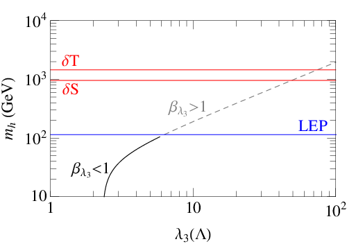

In Fig. 1, we display the dependence of the scalar-boson masses and on the quartic coupling , for which the Type-I flat-direction condition is realized. The solid (black) lines determine the perturbative region of the scalar-boson masses, which derive from the theoretical constraint, . The continuation of these lines into dashed (grey) lines correspond to the non-perturbative regime, in which . The area between the horizontal blue LEP line and the horizontal red line indicates the combined experimental limit on , i.e. . Similarly, the region above the horizontal red line is excluded by the limit. It is interesting to remark here that unlike the well-known “chimney plot” [25] which constrains the SM Higgs-boson mass to an allowed band by considerations of triviality and vacuum stability [26], Fig. 1 shows an exact value for the physical scalar masses against the quartic coupling which is related to the RG scale , see Fig. 2.
Fig. 2 shows the dependence of the RG scale on the quartic coupling . The same line colour convention as in Fig. 1 is used, only now the horizontal LEP, and lines are vertical. We observe that as approaches its minimum value, the coefficient gets close to zero, and so the RG scale tends to infinity. However, this area is not physically viable, as has already been excluded by the LEP limits.

If we interpret at the RG scale GeV as the most experimentally favourable value of this quartic coupling within the U(1)-invariant Type-I MSISM, we are then able to offer a sharp prediction for the masses of the heavier degenerate scalar bosons and . Specifically, by virtue of (5.2), we find that GeV. The fields and are both stable and can qualify as DM candidates in the so-called “Higgs-portal” scenario [24]. A detailed study of the DM relic abundances of and is beyond the scope of this paper and will be given elsewhere.
Since the -boson couplings to fermions and electroweak gauge bosons have exactly the SM form, its phenomenological distinction from the SM Higgs boson itself will be difficult. One possibility would be to look for the presence of large - and -couplings at the International Linear Collider (ILC), along the lines studied in [27]. Moreover, even though the trilinear and quadrilinear self-couplings are absent at the tree level, the large - and -couplings can give sizable contributions at the one-loop quantum level. Therefore, precision Higgs experiments at the ILC might be able to distinguish the MSISM from the SM.
From the analysis given above, it is clear that in spite of being very predictive, the U(1)-invariant Type-I MSISM has a number of weaknesses. This scenario satisfies all experimental limits for a large quartic coupling , which is close to the boundary of non-perturbative dynamics. Another problematic feature is that it exhibits a Landau pole at energy scales of order GeV, which is many orders of magnitude below the standard GUT ( GeV) and Planck ( GeV) mass scales. Therefore, in the next section, we relax the constraint of U(1) invariance, and investigate whether a general Type-I MSISM can be perturbative up to the GUT and Planck scales.
5.2 The U(1) Non-Invariant Scenario
We now lift the constraint of U(1) invariance from the scalar sector of the Type-I MSISM. The tree-level scalar potential of the general Type-I MSISM then reads:
| (5.5) | |||||
Exactly as we did for the U(1)-invariant scenario, we can show that the tree-level scalar-boson masses and the RG scale do not depend on all the couplings but only on and the modulus of the generally complex quartic coupling . In order to show this, we first notice that by substituting and into the squared scalar-boson mass matrix given in (B.9), we obtain only three non-zero matrix elements, i.e.
| (5.6) |
If is complex, the scalar-pseudoscalar mass term, , gives rise to explicit CP violation. In this case, the scalar mass spectrum consists of the fields:
| (5.7) |
If the theory preserves CP, we have that and are CP-even and CP-odd scalar fields, respectively. In the general case, however, the mass eigenstates have indefinite CP parities, with their tree-level masses given by
| (5.8) |
where . Hence, the scalar-boson masses depend on only two coupling parameters, and . For the same reason, the two effective potential coefficients and also depend on and through the scalar-boson masses . It is therefore not difficult to see that the one-loop induced -boson mass and the RG scale also depend only on and , by means of (4.20) and (4.21).
The fact that the scalar-boson masses have to be positive leads to the constraint:
| (5.9) |
This constraint automatically enforces the second condition in (4.6) for any value of , such that the potential remains BFB, i.e. , for . The first BFB condition in (4.6) is only fulfilled, if . This restricts the allowed parameter space of the other couplings, , and . In order for the first BFB condition to hold for any possible value of the phase , we must require that
| (5.10) |
As in the U(1)-invariant scenario, we may derive additional theoretical limits on and , by demanding that the couplings remain perturbative at and that the one-loop effective potential is BFB. The best theoretical upper limit on and is obtained by requiring that at and assuming that , and are negligible. This implies that
| (5.11) |
Correspondingly, a lower theoretical limit may be obtained by requiring that , which translates into the constraint:
| (5.12) |
Experimental data encoded as constraints on the electroweak oblique parameters , and provide complementary limits on the quartic couplings and . Exactly as in the U(1)-invariant scenario, only the boson interacts with the SM particles, with couplings of the SM form. Therefore, as before, useful perturbative constraints on and can only be derived from the 95% CL interval of the electroweak oblique parameters and for GeV. Since the boson has standard interactions, the LEP2 lower limit on the SM Higgs boson applies in full, giving rise to the constraint:
| (5.13) |


In Fig. 3 we present numerical estimates for the scalar-boson masses (upper panel), (middle panel) and (lower panel), as functions of the quartic coupling , after incorporating all the aforementioned theoretical and experimental limits. The perturbative areas which also contain positive scalar masses (5.9) are given by the white regions between the black lines, whereas their non-perturbative extrapolations are shaded grey with black dashed border lines. The LEP2, and limits are shown as the blue and two red lines, respectively. The areas to the right of the and lines are excluded by the respective 95% CL limits on and . Just like the U(1)-invariant scenario, the experimentally permitted regions lie between the LEP and lines, for quartic couplings which are slightly outside the boundary of perturbative dynamics. From the middle and lower panels of Fig. 3, we see that the preferred values of the and masses which correspond to GeV are constrained to lie in the intervals:
| (5.14) |
As in the U(1)-invariant scenario, the distinction of the Higgs sector of the general Type-I MSISM from that of the SM might require precision Higgs experiments at the ILC.
In Fig. 4 we display the dependence of the RG scale on the quartic coupling and include both the theoretical and experimental limits, using the same line colour convention as in Fig. 3. From Fig. 4, we see that the RG scale is of the electroweak order, lying in the range: GeV, for perturbative couplings, once the LEP2 Higgs-boson mass limit is taken into account.

In the general Type-I MSISM, the boson is a stable particle in all the allowed range of the quartic couplings. Therefore, it can represent a viable cold DM candidate, provided the boson is sufficiently massive, e.g. for GeV. If is small, then it opens a new decay channel for the SM-like Higgs boson via and for certain regions of parameter space can be the dominant mode of decay over when . However, for , the -boson decay into or still dominates. In addition to the boson, the heaviest boson might also become a stable particle and so a valid DM candidate, if its decay via the quartic interaction is kinematically forbidden, i.e. as long as .
The general CP-violating Type-I MSISM shares the same weakness as the U(1)-invariant Type-I MSISM. It turns out that it also generates a Landau pole at a maximum of GeV, far below the GUT and Planck scales. Unlike the U(1)-invariant scenario, the general model contains new sources of CP violation, which might be of particular importance for realizing electroweak baryogenesis. However, one serious drawback of the Type-I MSISM is that it cannot provide a natural implementation of the seesaw mechanism. Since the VEV of the complex singlet scalar vanishes, i.e. , no Majorana mass terms can be generated in this scenario. We therefore turn our attention in the next section to the Type-II MSISM, where .
6 The Type-II MSISM
In this section we study the MSISM that realizes a Type II flat direction along which both the Higgs doublet and the complex singlet scalar develop non-zero VEVs. We investigate the Type-II MSISM in two distinct cases: (i) the U(1)-invariant limit and (ii) a U(1) non-invariant scenario where CP is maximally broken spontaneously along the flat direction . For these two scenarios, we determine the perturbative values of the quartic couplings of the potential and the limits that these set on the scalar mass spectrum. Once these limits are considered, we find that the electroweak oblique parameters , and give no further constraints on the model parameters. On the other hand, as we will see, the LEP2 Higgs-boson mass limit does produce useful limits on the quartic couplings and the scalar-boson mass spectrum. Unlike in the Type-I MSISM, the pseudo-Goldstone boson in the Type-II case is in general a linear composition of all the neutral fields , and . As a consequence, it is possible for all the Higgs mass eigenstates , or to couple to the boson, but with reduced strength compared to the SM Higgs-boson coupling.
6.1 The U(1) Invariant Limit
In the U(1) invariant limit, the Type-II MSISM tree-level potential takes on the simple form:
| (6.1) |
Imposing the minimization conditions (4.11) and (4.12) on the tree-level potential (6.1), one gets a minimal flat direction at a given RG scale , provided the following relations among the VEVs of the scalar fields and quartic couplings are simultaneously met:
| (6.2) |
where we have made use of the U(1) symmetry to set the VEV of the field real. Hence, the flat direction becomes a two-dimensional vector with components and , given by (4.15). Moreover, as stated after (4.14), the quartic couplings should lie in the ranges: , and .
The flat direction relation (6.2) may be used to reduce the number of independent quartic couplings at to two, i.e. and . Instead, the quartic coupling may eliminated in favour of the relation: . Consequently, the scalar masses and the RG scale can be expressed entirely in terms of and . Taking the relations (6.2) into account, the scalar mass matrix given in (B.9) has the following non-zero entries:
| (6.3) |
We note that the U(1)-invariant Type-II MSISM cannot realize CP violation in the Higgs sector. Explicitly, the scalar mass spectrum consists of the mass eigenstates
| (6.4) |
where . The and bosons are CP even and the boson CP odd. The CP-odd scalar is the massless Goldstone boson, associated with the spontaneous symmetry breaking of the U(1) symmetry. At the tree-level, the only massive scalar is the boson, whose mass squared is given by
| (6.5) |
Since depends solely on the combination , so do the two effective potential coefficients and . Likewise, the RG scale also depends on the combination , through (4.21). However, the one-loop contribution to , given in (4.20), depends on as well, through the flat direction component , given in (4.15). Thus, the Higgs sector of the U(1)-invariant Type-II MSISM depends on and , or equivalently on and .


The full theoretical and experimental limits on the two quartic couplings and are displayed in Fig. 5. The top panel displays the full range, whilst the lower panel focuses on a very narrow region, which is viable for very small values of . As theoretical constraints, we require that the model remains perturbative at the RG scale , i.e. , which is represented by the black lines in Fig. 5. From these considerations, we find the upper limits and . Another useful theoretical constraint is obtained by requiring that the one-loop effective potential remains BFB ():
| (6.6) |
which is indicated by the black lines in Fig. 5. Thus, the theoretically admissible region is the one enclosed by the , and lines in the upper panel and by the , and lines in the lower panel.
The - parameter space may be further constrained by experimental LEP2 limits on the Higgs-boson mass and by the electroweak oblique parameters , and . We find that the 95% CL limits on , and parameters provide no additional constraints on the theoretically admissible region. Instead, the LEP2 Higgs-boson mass limits significantly restrict the - parameter space. To properly derive these limits, we first observe that the pseudo-Goldstone boson and the heavy -boson interact with reduced couplings and with respect to the SM coupling of to a pair of vector bosons . The squared reduced couplings and are given by
| (6.7) |
satisfying the identity: . Since the reduced -coupling can be much smaller than the SM one, the SM Higgs-boson mass limit GeV no longer applies. Instead, we use the combined constraints on and the scalar mass , which are presented in Fig. 10(a) of Ref. [5]. We perform a polynomial fit up to order 10 on the LEP2 data to obtain a reliable constraint on , which in turn restricts the - parameter space. This constraint is represented by the blue (grey) LEP line in the upper (lower) panel of Fig. 5, where the blue (grey) shaded region respect both the theoretical constraints and the LEP2 Higgs-mass limit. As there are two distinct shaded regions blue and grey, which correspond respectively to higher and lower values of , we shall consider each scenario separately.
6.1.1 The Electroweak Mass -Boson Scenario
We first consider the higher mass -boson scenario represented by the shaded blue area in Fig. 5, which is dominated by large values of and . In Fig 6 we show the dependence of the scalar boson masses and on the quartic coupling . The areas enclosed by the black lines are the regions which respect the theoretical constraints i.e. , and . Including the LEP2 Higgs-mass limit, we obtain the shaded blue areas, corresponding to an electroweak mass boson, with mass in the range: , and a rather heavy boson, with mass in the interval: . In addition, the gray shaded areas correspond to a very light boson, which is not clearly visible on the lower frame of Fig. 6, as it follows the line. This ultra-light -boson mass scenario will be discussed in more detail in Subsection 6.1.2.


The electroweak mass boson could be detected at the CERN Large Hadron Collider (LHC), through the decay channel . The observation of the boson may proceed via the so-called “golden channel,” . However, in the region , we have , on account of (6.7), which means that both decays will give reduced signals compared to the SM Higgs signals. Moreover, the heavier boson may predominantly decay invisibly into a pair of U(1) Goldstone bosons [28], thanks to the relatively large quartic couplings. This last characteristic makes the U(1) Type-II MSISM distinguishable from the corresponding Type-I one.

In Fig. 7 we present the dependence of the RG scale as a function of the quartic coupling . The area within the black lines respects the theoretical constraints, , the effective potential BFB condition and . The areas which also respect the LEP2 limit are shaded blue, which correspond to the electroweak -boson scenario, and grey, which correspond to a scenario with a very light boson. The latter region is very narrow and not clearly visible in the figure, since it very closely follows the line. If and are in the blue shaded region and remain perturbative, then the RG scale is of the order of the EW scale and lies in the range GeV. The region of the parameter space that remains perturbative to GUT or Planck scales lies firmly in the region excluded by the LEP2 limit. Taking this limit into account, the theory becomes non-perturbative at energies GeV, with a Landau pole at around GeV.
6.1.2 The Ultra-Light -Boson Scenario
Another experimentally and theoretically viable region of the - parameter space corresponds to a very small quartic coupling , giving rise to an ultra-light boson. The relevant region is shaded grey in the lower panel of Fig. 5. We will not present a detailed phenomenological analysis of this scenario, but rather highlight its key features.
As can be seen from Fig. 5, the LEP2 Higgs-mass limit puts an upper bound on . In view of this upper bound, the largest -boson mass is , as illustrated by the grey shaded region in Fig. 6. In this ultra-light -boson scenario, the reduced -coupling is rather suppressed, with , as can be determined from (6.7). This fact renders the boson difficult to detect at the LHC.
The other CP-even boson has almost a SM-like coupling to the vector bosons, with . Its mass may range for perturbative values of , between . This range is given by the line in Fig. 6. Since the -coupling is proportional to the small coupling it is suppressed and the SM-like boson would most likely be detected via the “golden channel,” .
An interesting feature of the ultra-light -boson scenario is the existence of a region that remains perturbative to higher scales than the previously considered models. This is indicated by the area enclosed by the solid and dashed green lines in Fig. 5. Specifically, within the allowed region, the model becomes non-perturbative at energies of order and develops a Landau pole at energies , which is higher than the electroweak mass -boson scenario. In conclusion, it worth reiterating that the U(1)-invariant Type-II MSISM has no new source of CP violation beyond the standard Kobayashi–Maskawa (KM) phase [29] and predicts no massive DM candidate (cf. Table 1). In spite of these drawbacks, the model does have the ability to generate Majorana neutrino masses through the seesaw mechanism, as we will discuss in more detail in Section 7. In the following section, we consider a minimal U(1)-violating Type-II MSISM which realizes maximal spontaneous CP violation (SCPV).
6.2 Minimal U(1) Non-Invariant Model of Maximal SCPV
Without the restriction of U(1) invariance, the tree-level scalar potential (4.2) of the general Type-II MSISM contains a total of 9 real quartic couplings which results in a multitude of valid solutions that all satisfy the minimization requirements (4.11) and (4.12). However, not all of these possible cases are phenomenologically interesting. Therefore, we have focused our investigation on a single U(1) non-invariant scenario that minimally realizes maximal spontaneous CP violation, i.e. it has a flat direction along the field line. The tree-level scalar potential of such a scenario is given by
| (6.8) |
where and is real as a consequence of CP invariance. In addition to CP symmetry, the tree-level scalar potential (6.8) is invariant under the discrete symmetry: and , with . The CP symmetry and the discrete symmetry are sufficient to uniquely fix the form of the tree-level scalar potential given in (6.8).
Minimizing the tree-level potential at the RG scale , by means of (4.11) and (4.12), we find the following relations for the flat direction:
| (6.9) |
Note that the second (or third) condition implies a flat direction that triggers maximal spontaneous CP violation with . Combining (6.9) with the BFB condition (4.6) requires that , and , where the signs of and individually remain undetermined. Another choice of a maximally CP-violating flat direction would be to have , i.e. . However, such a choice does not affect the scalar masses or the phenomenology of the model in an essential manner.
Other solutions to the minimization conditions, (4.11) and (4.12), are possible but they either reduce the potential to the U(1) invariant scenario () or modify it to a Type I flat direction (), both of which have been previously investigated in Sections 6.1 and 5, respectively.
The flat direction for this model can be expressed as a 3-dimensional vector, with non-zero , and components, i.e.
| (6.10) |
Considering the relations (6.9), the scalar mass matrix elements in (B.10) become
| (6.11) |
Note that the elements and are CP-violating. In terms of the quantum fields , and , the mass eigenstates , and are given by
| (6.12) |
Correspondingly, their tree-level masses squared are given by
| (6.13) |
where we employed the relation , as can easily be derived from (6.9). In order for the -boson mass squared to be positive, we require that , implying .
The Higgs sector of the Type-II MSISM of maximal SCPV depends on the three quartic couplings: , and . The quartic coupling can be eliminated in favour of , by means of (6.9). Explicitly, the scalar masses and depend on the three quartic couplings , as can be seen from (6.13). Likewise, the RG scale determined in (4.21) depends on the effective potential coefficients and that are both functions of and . Finally, according to (4.20), the pseudo-Goldstone boson depends on and . Nevertheless, from (6.10), we see that . Consequently, the entire scalar-boson mass spectrum of the model only depends on the three quartic couplings .
We may now exploit the extra freedom of the three independent quartic couplings to identify theoretically and experimentally viable regions of the parameter space which remain perturbatively renormalizable up to Planck-mass energy scales. To be precise, we require that and impose the tree-level BFB conditions up to the Planck scale: , and . Moreover, if we assume , such that we find that the quartic couplings are restricted to the intervals,
| (6.14) |
for . From (6.13), we observe that in the limit , the -boson mass becomes infinite. Therefore, to obtain an upper limit on , we require that the coefficients and of the one-loop effective in (4.17) are small, e.g. , such that perturbative unitarity in the Higgs sector holds true [30]. In our numerical analysis, we apply the constraint , which is comparable to the constraint . For definiteness, we choose two representative values of : and .


| min | max | min | max | min | max | min | max | |
|---|---|---|---|---|---|---|---|---|
| 0.2 | 54 | 78 | 155 | 181 | 783 | 1110 | 490 | 675 |
| 0.1 | 34 | 56 | 155 | 180 | 703 | 1110 | 444 | 674 |
| 0.05 | 21 | 39 | 154 | 179 | 607 | 1110 | 395 | 674 |
| 0.02 | 11 | 25 | 154 | 178 | 515 | 1110 | 350 | 675 |
In Fig. 8 we present numerical estimates of the scalar-boson masses, , , and the RG scale , as functions of the the quartic coupling . The solid and dashed black line enclose the regions permitted by considering the theoretical bounds which most tightly constrain the values of namely, , and , for and 0.02, respectively. The solid (dashed) blue lines represent the LEP2 Higgs-boson mass limit, which has been applied directly to the -boson mass for (0.02). The regions below the blue LEP lines are excluded for the specific values of considered. As a result, the coupling has to take small absolute values, with . The solid (dashed) red lines represent the theoretical limit for , where the area above the lines is excluded. The grey shaded regions are the areas which respect all the theoretical constraints and the LEP2 limit. Finally, the electroweak oblique parameters offer no useful constraints, within the theoretically allowed parameter space. In Table 2, we present the upper and lower limits on the masses of the and bosons and on the RG scale for different values of . The lower bounds are determined from the LEP2 Higgs-mass limit, whilst the upper bounds come from the theoretical constraint .
In Fig. 9 we display numerical estimates of the -boson mass as a function of the coupling. The black lines correspond to values of the quartic couplings which respect the limits , and . Even though the -boson mass evaluated in (6.13) does not explicitly depend on , the LEP2 limit applied to and the theoretical constraint do, as can be seen from Table 2. The grey shaded areas between the solid (dashed) blue LEP and red lines are allowed by the respective constraints for (0.02). The LEP2 limit provides an upper limit on the value of , whilst the constraint gives a lower limit. These upper and lower limits on the -boson mass are exhibited in Table 2, for various values of the coupling.


In spite of the additional quartic coupling , the interactions of the and scalars to a pair of bosons are very similar to the U(1)-invariant scenario. The reduced - and -couplings are given by
| (6.15) |
In the Type-II MSISM of maximal SCPV under study, the boson has a large component from the heavy scalar and so it can generically be heavier than the respective in the U(1)-invariant model, this allows it to comfortably evade detection at the LEP2. On the other hand, the boson has a SM-like coupling to the electroweak vector bosons and would again most likely be detected through the standard discovery channel . In addition to the standard discovery channel, , the boson may now decay favourably to a pair of bosons, i.e. , if kinematically allowed. Then, each of the bosons may decay into a pair of leptons or quarks. A detailed phenomenological study of this detection channel for the LHC is beyond the scope of this paper.
The minimal Type-II MSISM of maximal SCPV gives rise to rich phenomenology. As mentioned previously, the model spontaneously and maximally violates the CP symmetry. Since the complex singlet has a non-zero VEV, the model can also generate naturally small neutrino masses through the seesaw mechanism. Moreover, the presence of a permutation parity symmetry, , which remains intact after EWSSB, renders the massive boson stable, with vanishing VEV. Hence, the boson could act as a cold DM, according to the Higgs-portal scenario [24]. In general, there are two parity symmetries that could be imposed on a general Type-II MSISM with SCPV, they are: and . Both symmetries lead to similar mass spectra, so we do not discuss them separately. Also, both symmetries trigger maximal SCPV, which might open up the possibility for successful electroweak baryogenesis in this scenario.
In summary, the Type-II MSISM of maximal SCPV is a theoretically and experimentally viable scenario. The quartic couplings of the model can remain perturbative up to Planck energy scales and its scalar-boson spectrum is compatible with limits from LEP2 Higgs searches and the , and oblique parameters. Most importantly, the model does not require additional theory to stay perturbatively renormalizable up to the standard quantum gravity scale, i.e. . Since the addition of right-handed neutrinos can have a significant impact on the one-loop effective potential and on the phenomenology of the model in general, we analyze in detail such a scenario in the next section.
7 The MSISM with Right-Handed Neutrinos
In order to account for the observed non-zero neutrino masses, we extend the MSISM with three right-handed neutrinos, . As was already mentioned in Section 4.4, the Type-I MSISM cannot realize the seesaw mechanism since the VEV of the field is zero along the minimal flat direction. The only way of introducing neutrino masses in a SI fashion into the Lagrangian is through the hugely suppressed neutrino Yukawa couplings of order , which are about 6 orders of magnitude smaller than the electron Yukawa coupling. Obviously, such a scenario has the difficulty of naturally explaining the smallness of the light neutrino masses. Moreover, the Type-I MSISM with right-handed neutrinos is a highly uninteresting scenario as the actual effect of the very small neutrino Yukawa couplings on the scalar potential is negligible.
We therefore turn our attention to the Type-II MSISM. The Lagrangian term in (4.1), which describes the dynamics of the right-handed neutrinos, is given by
| (7.1) | |||||
where the usual summation convention over repeated indices is implied, with labelling the three generations, , and , respectively. In (7.1), are the Dirac-neutrino Yukawa couplings of the SM Higgs doublet to the lepton doublets , as defined in Appendix A. In addition, and are the two possible Majorana-neutrino Yukawa couplings of the singlet field to the right-handed neutrinos . Note that and are symmetric matrices, i.e. , . Since the Majorana-neutrino Yukawa couplings and can be sizeable, we need to calculate their effect on the flat-directions and the one-loop functions. Technical details of such calculations are given in Appendices B and C.
Since along the Type-II flat direction, the following neutrino mass terms are generated:
| (7.2) |
with
| (7.3) |
Without loss of generality, we can assume a weak basis, in which is diagonal, real and positive, whilst , and are in general non-diagonal complex matrices.
The mass matrix in can be block-diagonalized via a unitary matrix as follows:
| (7.4) |
To leading order in an expansion in powers of , we obtain the standard seesaw formulae:
| (7.5) |
where is a light neutrino mass matrix pertinent to the masses of the observed light neutrinos and is the heavy neutrino mass matrix, predicting new heavy Majorana neutrinos, which we denote hereafter as .
As we will see in this section, the heavy Majorana neutrinos in the Type-II MSISM are typically not much heavier than the EW scale. In the standard seesaw framework [22], all Dirac-neutrino Yukawa couplings have to be less than about , e.g. of order the electron Yukawa coupling. However, the possible presence of approximate flavour symmetries in and/or [31, 32, 33] are sufficient to relax this constraint for some of the Dirac-neutrino Yukawa couplings and render them sizeable of order –1 [34, 35]. Even though we keep the analytic dependence of our results on , we assume that all , such that their numerical impact on the one-loop effective potential and the electroweak oblique parameters can be safely ignored.
In the following, we study several representative scenarios within the framework of the Type-II MSISM with right-handed neutrinos. First, we consider a U(1)-symmetric theory that preserves the lepton number. We then consider a benchmark scenario of Type-II MSISM with maximal SCPV and analyze two variants of such a scenario. The first variant assumes a CP-symmetric neutrino Yukawa sector, where the CP invariance is only violated spontaneously by the ground state of the theory. The second variant promotes a parity symmetry present in the scalar potential of the model to the neutrino Yukawa sector, thus giving rise to a massive stable scalar particle. This stable scalar particle could act as a potential candidate to solve the cold DM problem.
7.1 Neutrinos in the U(1) Invariant Type-II MSISM
We now consider the effect of including right-handed neutrinos in the the U(1)-invariant Type-II MSISM. The imposition of U(1) symmetry on the neutrino Yukawa sector is equivalent to lepton-number conservation, where the right-handed neutrinos carry the lepton number and the singlet field the lepton number . As a consequence of lepton-number conservation, the Majorana Yukawa coupling vanishes and the heavy-neutrino mass matrix along the Type-II flat direction is given by
| (7.6) |
where we have set by virtue of a U(1) rotation.
With the aid of (6.2), we may now express the light- and heavy neutrino mass matrices, and , in terms of the SM VEV :
| (7.7) |
where is a real and diagonal matrix. For simplicity, we assume that three heavy Majorana neutrinos are nearly degenerate, specifically by assuming that is SO(3) symmetric. The perturbativity constraint on the Yukawa couplings may be translated into the inequality, , at the RG scale . This constraint leads to the upper bound, , for a perturbative theory up to the EW scale. If we insist that the Majorana Yukawa couplings stay perturbative up to the Planck scale, we find the tighter upper limit: . Finally, the condition that the one-loop scalar potential be BFB, i.e. , along with the perturbativity conditions, , yield the upper limit on , , at the EW scale.

Fig. 10 shows the allowed parameter space of the -boson mass and the Majorana-neutrino Yukawa coupling , compatible with the LEP2 Higgs-mass limit. The maximum perturbative value is represented by the black line, such that the area between the black line and the line corresponds to perturbative masses. The maximum perturbative value for depends on the perturbatively allowed values for , and , i.e and . Since right-handed neutrinos induce a negative contribution to the coefficient defined in (4.18) and so to in (4.20), decreases as the right-handed neutrino Yukawa coupling increases. In Fig. 10, the areas which are permitted by the LEP2 Higgs-mass limit are shaded blue and grey, for the electroweak mass and the ultra-light -boson scenarios, discussed in Subsections 6.1.1 and 6.1.2, respectively. In the electroweak mass -boson scenario, where , the Majorana-neutrino Yukawa coupling is restricted to be: . Instead, for the ultra-light boson scenario (with ), we get the upper limit: . In this context, the influence of the Majorana-neutrino Yukawa coupling on the RG scale is not significant, as we find GeV for . We also verified that all values of and which respect lie within the 95% CL interval of , and , using the limits for GeV.
In Fig. 11 we display the allowed parameter space of and , for all perturbative values of and , under the constraint: . The allowed space is given by the area enclosed by the two black lines. The blue and grey shaded areas indicate the parameter space which is allowed by the LEP2 Higgs-boson mass limit. As can be seen from Fig. 11, the resulting allowed areas set upper limits on the heavy Majorana neutrino masses, GeV and GeV, for the electroweak and the ultra-light -boson scenarios, respectively. Depending on the strength of the neutrino Yukawa couplings , such heavy Majorana neutrinos can be produced at the LHC [36], leading to like-sign dilepton signatures without missing energy.

As was discussed in Section 6.1, the U(1)-invariant Type-II MSISM predicts no massive stable scalar particle that could play the role of the cold DM. In fact, the presence of the Majorana neutrinos, and , leads to new decay channels for the scalar particles and , such as and [32]. Moreover, the inclusion of right-handed neutrinos does not change the UV behaviour of the model which becomes non-perturbative and develop a Landau pole far below and . For this reason, we turn our attention to the Type-II MSISM of maximal SCPV, which does not exhibit this weakness.
7.2 Neutrinos in a Minimal Model of Maximal SCPV
We now consider an extension of the Type-II MSISM presented in Section 6.2, by adding right-handed neutrinos. The Type-II flat direction of this scenario is given by , which leads to maximal SCPV in the one-loop scalar potential. Along this flat direction, the heavy Majorana neutrino mass matrix takes on the form:
| (7.8) |
Since the Majorana Yukawa couplings, and , may contain large number of independent parameters, we will investigate two simple variants of the model. In the first variant, we assume that both and are real, i.e. there is no sources of explicit CP violation in neutrino Yukawa sector. The second variant makes use of a parity symmetry, which gives rise to a massive stable scalar particle that could qualify as DM.
7.2.1 The CP Symmetric Limit
In the CP symmetric limit of the theory, the Yukawa couplings and are all real. In the weak basis, where is real and diagonal, one then gets the constraint: . Implementing this last constraint along the Type-II flat direction , the neutrino mass matrices read:
| (7.9) |
Assuming a universal scenario with three degenerate heavy neutrinos, with , the coupling parameter has to be less than to be perturbative at the RG scale . This perturbativity constraint becomes stronger at the GUT and Planck scales, where we obtain the upper limits, and , respectively.
This model depends on four independent theoretical parameters, namely , (or ), and . As particular viable benchmark models, we consider the following three cases:
| (7.10) |


In Fig. 12 we present the allowed parameter space in the - plane, for the Cases A, B and C given in (7.10). The area between the black lines is allowed by the considerations: , and in Case B or in Cases A and C, which give the tightest theoretical constraints for the model to remain perturbative to the Planck scale. Furthermore, the area above the red line is excluded, because it violates perturbative unitarity in the MSISM Higgs sector [30]. For Case A and C, the line is above the allowed region and has not been displayed. We find that, within the theoretically allowed areas, the predictions for the electroweak oblique parameters , and fall within the 95% CL intervals for the three scenarios considered. The region below the grey dashed line is excluded by the LEP-2 Higgs-mass limit applied to the -boson mass . As a consequence, the grey shaded areas correspond to the regions which are allowed by our theoretical considerations and the LEP2 and oblique paameters. The presence of the right-handed neutrinos does not greatly affect , except when approaches its maximum allowed value which reduces the prediction for , as shown in Fig. 12. The other scalar masses, , are not affected by the inclusion of neutrinos, since they are independent of at the tree level.


Fig. 13 displays the allowed parameter space spanned by the Majorana-neutrino Yukawa coupling and the universal right-handed neutrino mass for the three benchmark scenarios listed in (7.10). As before, the area between the black lines is permitted by the considerations: , and in Case B or in Cases A and C, and the area above the red line violates perturbative unitarity, and so it is theoretically inadmissible. The area below the grey dashed LEP line is excluded by LEP2 Higgs-mass limit applied the . The grey shaded region is permitted by theory and the LEP2 limit. Comparing the three cases, we observe that if decreases or increases, both the upper limits on and increase. From Fig. 8, we see that if increases also needs to increase to remain within the theoretical and LEP2 limits and so the two effects cancel and we assume the maximal values of and do not vary significantly from the values given in Case B. Within this benchmark scenario, we can then derive approximate upper limits on the values of and . Thus, from the middle panel of Fig. 13, we observe that the heavy Majorana neutrinos can generically have masses up to TeV scale, i.e. , and must remain relatively small in order for the one-loop effective potential to be BFB, i.e. .
The only weakness of the present model under study is that the would-be DM candidate, the boson, is no longer stable, since it can decay to , where is an off-shell heavy Majorana neutrino, which can subsequently decay into off-shell and bosons and charged leptons and light neutrinos. The decay of the boson is a consequence of the violation of the parity symmetry, , in the Majorana-neutrino Yukawa sector. In the following, we consider a minimal Type-II MSISM, where the parity symmetry is elevated to an exact global symmetry acting on the complete Lagrangian of the theory.
7.2.2 The Boson as a Cold DM Candidate
As mentioned above, in the absence of right-handed neutrinos, the scalar potential of the Type-II MSISM with maximal SCPV possesses the permutation symmetry: . Under the action of this symmetry, the scalar field is odd: . This parity symmetry remains unbroken after the EWSSB, leading to a massive stable scalar particle, which could play the role of the cold DM in the Universe.
We may now extend the above permutation or parity symmetry to neutrino Yukawa sector of the model, which implies that . As a consequence, the boson will not interact with the neutrinos, so it will remain a massive stable particle which can potentially act as DM particle. Given the relation , the light- and heavy-neutrino mass matrices become
| (7.11) |
where in the weak basis, in which is real. Assuming a universal Majorana flavour structure with , we find that must be less than 2.1 in order to be perturbative at the RG scale and less than 0.37 and 0.33 to remain perturbative at the GUT and Planck scales, respectively.


Fig. 14 shows the allowed parameter space of the -boson masses and the real part of the Majorana Yukawa coupling , for the three Cases A, B and C defined in (7.10). The area enclosed by the black lines is theoretically favoured by the perturbative and BFB conditions: , and which offer the tightest theoretical constraints. Instead, the area above the red line is disfavoured, because it violates perturbative unitarity in the Higgs sector. Above the grey dashed LEP lines correspond to the regions which are also permitted by the LEP2 Higgs-mass limit applied to , whereas constraints from the , and parameters play no role in the theoretically allowed parameter space. The grey shaded regions are theoretically and experimentally permitted. From Fig. 14, we observe that the -boson mass has a similar range of values as the CP-symmetric MSISM discussed in the previous subsection.
In Fig. 15 we display the allowed parameter space of the universal right-handed neutrino Majorana mass and , for the three different Cases A, B and C. As before, we consider the following theoretical conditions: , , and . The theoretically favoured regions are those, which are enclosed by the black , and BFB () lines. The grey shaded areas correspond to the regions which are also permitted by the LEP2 Higgs-mass limit applied to . In all the three benchmark scenarios considered, the heavy Majorana neutrino mass scale stays below the TeV scale and the value of is constrained to be: .
In summary, the variant of the Type-II MSISM with maximal SCPV and right-handed neutrinos we discussed in this subsection has a number of physically interesting properties. First, it can realize a parity symmetry in the theory, such that the boson becomes a stable particle and so could play the role of the cold DM in the Universe. Second, the present model can implement an electroweak seesaw mechanism to provide naturally small neutrino masses. It contains a new source of spontaneous CP violation, thereby enabling us to address the problem of the baryon asymmetry in the Universe. The model successfully passes all obvious experimental constraints from LEP2 Higgs and other electroweak precision data. Finally, of particular interest is the existence of a significant region of the theoretical parameter space, within which the model can stay perturbative up to Planck-mass energy scales.
8 Conclusions
We have performed a systematic analysis of an extension of the Standard Model that includes a complex singlet scalar field and is scale invariant at the tree level. We have called such a model the Minimal Scale Invariant extension of the Standard Model (MSISM). Quantum corrections explicitly break the scale invariance of the classical Lagrangian of the model and may trigger EWSSB. Even though the scale invariant SM is not a realistic scenario, the MSISM may result in a perturbative and phenomenologically viable theory that may potentially solve the gauge hierarchy problem.
We have presented a complete classification of the flat directions which may occur in the classical scalar potential of the MSISM. Employing the perturbative GW approach to EWSSB, we have calculated the one-loop effective potential along the different flat directions and derived the necessary and sufficient conditions for the scalar potential to be BFB [cf. (4.6)]. In addition, we have computed the scalar-boson masses, including theoretical constraints from the validity of perturbation theory, as well as phenomenological limits from electroweak precision data and direct Higgs-boson searches at LEP2.
The different flat directions in the MSISM can be classified in three major categories: Type I, Type II and Type III. In the Type-I MSISM, the singlet scalar has a zero VEV at the tree level, whereas in the Type-II MSISM both the VEVs of and the SM Higgs doublet are non-zero. In Type-III MSISM, the Higgs doublet has a vanishing VEV at the tree-level, which makes it somewhat difficult to naturally realize EWSSB. Therefore, our analysis has focused only on scenarios realizing Type-I and Type-II flat directions. We have found that the general Type-I MSISM is perturbative only up to the EW scale and exhibits a Landau pole at energy scales GeV. Likewise, we have found that the U(1)-invariant Type-II MSISM is perturbative up to energies GeV and develops a Landau pole at energy scales GeV. In this respect, our results are in qualitative agreement with [8]. As we have shown, however, this is not an indispensable property of a general Type-II MSISM. Moving away from the model-building constraint of U(1) invariance, we have explicitly demonstrated that a minimal Type-II MSISM of maximal SCPV can stay perturbative up to the Planck scale, without the need to introduce unnaturally large hierarchies between the scalar-potential quartic couplings, or between the VEVs of the and fields which may reintroduce an additional hierarchy problem.
In the present study, we have taken the view that the generation of the electroweak scale is the result of the breaking of the scale invariance of the Higgs sector of the MSISM. Instead, we have tacitly assumed that quantum gravity effects are small and do not destabilize the gauge hierarchy. As was argued in [9, 11], for example, the latter may be the consequence of a conformally UV complete theory of quantum gravity, which we are currently lacking. However, a necessary ingredient for such a theory to succeed appears to be the absence of any additional scale between and . It is therefore important that the quartic couplings remain perturbative up to the Planck scale, without the presence of a Landau pole which could introduce an additional unwanted higher scale in the theory, through non-perturbative effects that could dynamically break the scale invariance and so destabilize the gauge hierarchy.
We have investigated the phenomenological implications of the Type-I and Type-II MSISM, in particular, whether they realize explicit or spontaneous CP violation, neutrino masses or predict dark matter candidates. The key features of the different scenarios have been summarized in Table 1. To naturally account for the very small light-neutrino masses through the seesaw mechanism, we have extended the Type-II MSISM with right-handed neutrinos. Our analysis shows that the right-handed neutrino mass scale cannot be much higher than the TeV scale and so heavy Majorana neutrinos might lead to observable like-sign dilepton effects at the LHC. On the other hand, the addition of right-handed neutrinos generically renders all scalar fields unstable and so prevents them from acting as DM particles. However, we have shown that this problem could be solved by promoting a parity symmetry present in the scalar potential of the model to the neutrino Yukawa sector and to the complete Lagrangian. One of the scenarios satisfying this criterion is the Type-II MSISM of maximal SCPV.
There are several issues which are beyond the scope of the present paper, but need to be studied in greater detail. Specifically, it would be interesting to determine the precise constraints on the parameter space derived from the predicted DM relic abundances. Similarly, additional constraints may be derived from considerations of the baryon asymmetry in the Universe. Finally, it would be interesting to investigate, whether the presence of some of the quasi-flat directions in the MSISM could also serve to drive cosmological inflation. These are some of the issues that remain open within the MSISM, which we aim to address in the near future.
Acknowledgements
L. A-N. thanks the participants of the “Workshop on Multi-Higgs Models” in Lisbon, Portugal ( September 2009) for useful discussions.
Appendix A The Yukawa and Gauge Sectors of the MSISM
Here we briefly discuss the Yukawa and electroweak gauge sectors of the MSISM, which closely resemble the SM. This brief exposition will enable us to set up the notation and determine the gauge-dependent masses and couplings that enter our calculations for the effective potential, the anomalous dimensions and the electroweak oblique parameters.
The gauge-invariant part of the Lagrangian describing the Yukawa and electroweak gauge sectors is given by
| (A.1) | |||||
where , and are the field strength tensors of the SU(3)c, SU(2)L and U(1)Y gauge fields, (with ), (with ) and , respectively. Correspondingly, , and are the SU(3)c, SU(2)L and U(1)Y gauge couplings and is the covariant derivative defined as , where () are the usual Gell-Mann (Pauli) matrices and is the weak hypercharge of the various fields,
| (A.2) |
In (A.1), we have used to collectively represent all the fermions of the model,
| (A.3) |
where the subscripts and denote the left- and right-handed chiralities of the fermion. Each type of fermion has three generations represented by , i.e. . The matrices contain the Yukawa couplings for the SM up- and down-type quarks and charged leptons. Finally, we denote the hypercharge conjugate field of the Higgs doublet as .
A convenient gauge-fixing scheme to remove the tree-level mixing terms between the Goldstone and gauge bosons is the class of gauges. Adopting this scheme and decomposing linearly the neutral component of about its one-loop induced VEV, as , we may write the gauge-fixing and the induced Faddeev–Popov Lagrangians as follows:
| (A.4) |
where (), () and are the SU(3)c, SU(2)L and U(1)Y ghost fields, respectively, and
| (A.5) |
The would-be Goldstone bosons obtain gauge-dependent mass contributions due to the gauge fixing term , given by
| (A.6) |
Similarly, the ghosts also gain gauge-dependent mass eigenvalues from , i.e.
| (A.7) |
where , and .
We should note that after EWSSB, all -dependent masses and couplings affect the one-loop effective potential along the flat direction, but they do not influence the one-loop anomalous dimensions and functions, which may be computed in the symmetric phase of the theory. In the same context, we also note that the -dependent terms contribute to the electroweak oblique parameters, , and , which are conventionally calculated in the Feynman-’t Hooft gauge .
Appendix B The One-Loop Effective Potential of the MSISM
Here we calculate the one-loop effective potential of the MSISM. To this end, we use the functional expression [37, 38]:
| (B.1) |
where is the second derivative of the classical action , i.e.
| (B.2) |
In the above, collectively denotes each of the fields,
where is the classical field defined as the VEV of the operator in the presence of the source and for fields obeying the Bose–Einstein (Fermi–Dirac) statistics. Moreover, the trace in (B.1) acts over all space and internal degrees of freedom. For our purposes, a more convenient representation of (B.1) is
| (B.3) |
In momentum space of dimension, this last expression becomes
| (B.4) |
and now symbolizes the trace only over the internal degrees of freedom, e.g. over the polarizations of the gauge fields, the spinor components of the fermions or the Yukawa coupling matrices.
The one-loop effective potential of the MSISM can now be calculated by applying (B.4) to the scalars, gauge bosons (GB), ghosts, charged fermions (CF) and neutrinos (N) individually, i.e.
| (B.5) | |||||
For the scalar contribution, this is a non-trivial derivation, since as defined in (B.2) is the matrix:
| (B.6) |
Observe that and are matrices, and are complex numbers, and the remaining entries, e.g. etc, are two-dimensional complex vectors. This internal matrix structure needs be treated with care and must be preserved when determining the matrix, . Taking this fact into account, the scalar contribution is found to be
| (B.7) | |||||
where , is the Euler–Mascheroni constant and is ’t-Hooft’s renormalization scale. The Goldstone mass terms in the above equation are given by
| (B.8) |
These mass terms vanish along the flat direction because of (4.11). However, after EWSSB they obtain additional -dependent contributions through the gauge fixing terms [cf. (A.6)].
The masses appearing in (B.7) correspond to the eigenvalues of the matrix
| (B.9) |
where
| (B.10) |
Note that reduce to the squared mass terms for the , and fields, respectively, if all mixing terms between the scalar fields vanish along a given flat direction. In addition, we should remark here that one of the eigenvalues of the matrix (B.9) will always be zero along a minimal flat direction, since it corresponds to the pseudo-Goldstone boson of scale invariance.
We now turn our attention to the gauge-boson contribution in (B.5), which has been calculated in the gauge. The gauge-boson contribution reads:
| (B.11) | |||||
where
| (B.12) |
In the same class of gauges, the ghost contribution is given after EWSSB by
| (B.13) |
where and are the field-dependent ghost masses.
Next, we calculate the charged fermion contribution to the effective potential (B.5). This is given by
| (B.14) | |||||
where () are the eigenvalues of the background -dependent squared mass matrix for the -type fermion: . Note the factor 3 in front of the up- and down-type quark contributions which counts the SU(3)c colour degrees of freedom.
If the MSISM is extended with right-handed neutrinos, these will give rise to additional quantum effects on the one-loop effective potential (B.5). The contribution of the light and heavy Majorana neutrinos to the effective potential is given by
| (B.15) | |||||
where is the background - and -dependent light-neutrino mass matrix,
| (B.16) |
and is the respective -dependent heavy-neutrino mass matrix:
| (B.17) |
Finally, an important remark is in order. The one-loop effective potential is in general gauge dependent through (B.11) and after EWSSB through (B.13) and the Goldstone -dependent mass terms in (B.7) as well. However, it is known that the effective potential becomes gauge-independent when evaluated at local extrema [39, 40]. Within the context of perturbation theory, the one-loop effective potential should be -independent, if it is evaluated along a stationary flat direction [41]. This is exactly the case of the GW approach to the effective potential (3.8). Therefore, as a consistency check, we have verified that the -dependent terms due to gauge, Goldstone and ghost contributions cancel against each other in the effective potential (B.5) when evaluated along a stationary flat direction.
Appendix C One-Loop Anomalous Dimensions and -Functions
In this section, we calculate the one-loop anomalous dimensions of the fields and the functions of couplings in the MSISM, within the scheme of renormalization in the class gauges. Our calculation is based on the so-called displacement operator formalism, or -formalism in short, which was developed in [42] as an alternative approach to systematically performing renormalization to all orders in perturbation theory. Since this is not a common approach, we briefly review its basic features.
According to the -formalism, the renormalized one-particle irreducible -point correlation functions, denoted hereafter with a script , are related to the unrenormalized ones through:
| (C.1) |
where is the displacement operator that takes the form,
| (C.2) |
where again represents all the fields in the model, all the coupling constants, i.e. , and is the gauge fixing parameter. In addition, the counterterm renormalizations, , etc, are defined as, , etc.
We may now perform a loopwise expansion of the operator in (C.1),
| (C.3) |
where the superscript on denotes the loop order, i.e.
| (C.4) |
Correspondingly, the parameter or counterterm shifts and are loopwise defined as
| (C.5) |
Applying the -formalism to one-loop, we have
| (C.6) |
This last equation can be used to calculate the wavefunction and coupling constant renormalizations, and . Having thus obtained and , we may compute the one-loop anomalous dimensions of the fields and the functions of the couplings as follows:
| (C.7) |
where is the tree-level scaling dimension of the generic coupling in dimensions, with for the scalar quartic couplings, for the gauge and Yukawa couplings and for the gauge-fixing parameter. It is useful to remark here that the one-loop anomalous dimensions of the fields and the functions can be calculated in the symmetric phase of the theory.
Employing (C.6) and (C.7) in the scheme, we may calculate the one-loop anomalous dimensions and functions in the gauge. More explicitly, we obtain for the anomalous dimensions of the fields:
| (C.8) |
where and . Notice that and , where we have used and , which is a consequence of the Majorana constraint on the left-handed and right-handed neutrinos, and .
Correspondingly, we start by listing the one-loop functions of the scalar-potential quartic couplings:
| (C.9) | |||||
where . Note that the one-loop functions of the complex conjugate quartic couplings, i.e. , are given by .
For the one-loop functions of the SU(3)c, SU(2)L and U(1)Y gauge couplings, we use the well-established results:
| (C.10) |
Next, we present the known one-loop functions of the up-type and down-type quark Yukawa couplings
| (C.11) |
Finally, the one-loop functions of the light- and heavy-neutrino Yukawa couplings are calculated to be
| (C.12) | |||||
The one-loop anomalous dimensions and functions can be used to verify the renormalizability of . To be specific, the potential should be UV finite after renormalization. In the so-called renormalization scheme [43], the one-loop UV counter-terms for the fields and coupling constants are explicitly given by
| (C.13) |
Taking these relations into account, the one-loop MSISM effective potential can be renormalized in the scheme and its complete analytic form is given by
| (C.14) | |||||
where the mass terms are defined in Appendices A and B. Notice that along a stationary flat direction, and the -dependent Goldstone-boson masses and , given in (A.6), cancel against the -dependent contributions from the and bosons and their respective ghost fields. Hence, the complete one-loop renormalized effective potential becomes gauge independent in this case.
Appendix D The Electroweak Oblique Parameters
In order to calculate the electroweak oblique parameters , and , we adopt the notation and formalism developed in [18]. To this end, we first review the definitions of the , and parameters and present their basic relations with the gauge-boson self-energies, which we will then use to determine the electroweak oblique parameters in the MSISM.
In detail, the vacuum polarization amplitudes are defined as
| (D.1) |
where and
| (D.2) |
These vacuum polarizations are related to the one-particle irreducible self-energies of the , and gauge bosons through:
| (D.3) |
where is the electric charge and is the electroweak mixing angle. One can now solve the above system of linear equations for the vacuum polarization amplitudes and define the so-called electroweak oblique parameters [18] in terms of them as follows:
| (D.4) |
where is the electromagnetic fine structure constant. Noting the dependence of , and in (D.3), the , and parameters can be determined by calculating the and vacuum polarization amplitudes only.


Our interest is to find the difference in the predictions for the electroweak oblique parameters in the MSISM from the corresponding ones in the SM, i.e. , where . As shown in Figure 16, the main loop effect beyond the SM arises from the MSISM Higgs scalars and that occur in the and self-energies. The sum of these three diagrams for each one of the three scalar bosons, , and , is denoted as . Specifically, the shifts are due to the Higgs scalar masses and , as well as their modified gauge couplings and with respect to the SM coupling , where . Hence, the deviations of the electroweak oblique parameters may be obtained by
| (D.5) |
Here, the generic function stands for the functions , , and , which are defined as
| (D.6) | |||||
| (D.7) | |||||
| (D.8) | |||||
In the above, we have followed the standard convention and calculated the electroweak oblique parameters in the Feynman-’t Hooft gauge, in which and . Moreover, it is important to note that , and are UV finite and independent of , as it can be easily checked by means of the coupling sum rule: .
The theoretical predictions for , and in the MSISM are confronted with their experimental values [17]:
| (D.9) |
where the first uncertainty is evaluated by assuming that GeV, while the second one given in parenthesis should be added to the first to give the uncertainty for assuming GeV. Along with the LEP2 95% CL limit presented in Fig. 10(a) of Ref. [5], we also adjust the experimental limits on , and to give a corresponding 95% CL interval. The following limits have been implemented throughout our analysis:
| (D.10) |
For definiteness, we have chosen here the Higgs-mass reference value, , even though the derived constraints on the electroweak oblique parameters are independent of the choice of .
Finally, we should remark that we have not included the contributions of the light and heavy Majorana neutrinos, and , to the electroweak oblique parameters. These contributions are suppressed either by the smallness of the light neutrino masses or because they are proportional to , i.e. they are suppressed by the fourth power of the small neutrino Yukawa couplings. These contributions can therefore be safely neglected, when compared to the dominant scalar-loop effects on the , and parameters.
References
- [1]
S.L. Glashow,
Nucl. Phys. 22 (1961) 579;
S. Weinberg (1967). Phys. Rev. Lett. 19 (1967) 1264;
A. Salam, “Elementary Particle Physics Relativistic Groups and Analyticity,” ed. N. Svartholm (1968), Eighth Nobel Symposium; Stockholm: Almquvist and Wiksell, pp. 367. - [2]
F. Englert and R. Brout,
Phys. Rev. Lett. 13 (1964) 321;
P. W. Higgs, Phys. Rev. Lett. 13 (1964) 508;
G. S. Guralnik, C. R. Hagen and T. W. B. Kibble, Phys. Rev. Lett. 13 (1964) 585. - [3] S. R. Coleman and E. Weinberg, Phys. Rev. D 7 (1973) 1888.
- [4] E. Gildener and S. Weinberg, Phys. Rev. D 13 (1976) 3333.
- [5] R. Barate et al. (the ALEPH Collaboration, the DELPHI Collaboration, the L3 Collaboration and the OPAL Collaboration, The LEP Working Group for Higgs Boson Searches) Phys. Lett. B 565 (2003) 61.
- [6] R. Hempfling, Phys. Lett. B 379 (1996) 153.
- [7]
W. F. Chang, J. N. Ng and J. M. S. Wu,
Phys. Rev. D 75 (2007) 115016;
S. Iso, N. Okada and Y. Orikasa, Phys. Lett. B 676 (2009) 81. - [8] R. Foot, A. Kobakhidze and R. R. Volkas, Phys. Lett. B 655 (2007) 156.
- [9] K. A. Meissner and H. Nicolai, Phys. Lett. B 648 (2007) 312; Phys. Lett. B 660 (2008) 260.
- [10] K. A. Meissner and H. Nicolai, Eur. Phys. J. C 57 (2008) 493.
- [11] W. A. Bardeen, “On naturalness in the standard model”, preprint FERMILAB-CONF-95-391-T.
- [12]
G. ’t Hooft, Nucl. Phys. B 33 (1971) 173;
G. ’t Hooft and M. Veltman, Nucl. Phys. B 44 (1972) 189. - [13] R. Foot, A. Kobakhidze, K. L. McDonald and R. R. Volkas, Phys. Rev. D 77 (2008) 035006.
- [14] K. A. Meissner and H. Nicolai, Phys. Rev. D 80 (2009) 086005.
- [15] D. O’Connell, M. J. Ramsey-Musolf and M. B. Wise, Phys. Rev. D 75 (2007) 037701.
- [16] V. Barger, P. Langacker, M. McCaskey, M. J. Ramsey-Musolf and G. Shaughnessy, Phys. Rev. D 77 (2008) 035005; Phys. Rev. D 79 (2009) 015018.
- [17] C. Amsler et al. [Particle Data Group], Phys. Lett. B 667 (2008) 1.
- [18] M. E. Peskin and T. Takeuchi, Phys. Rev. Lett. 65 (1990) 964; Phys. Rev. D 46 (1992) 381.
- [19]
For an alternative formulation, see
G. Altarelli and R. Barbieri, Phys. Lett. B 253 (1991) 161;
G. Altarelli, R. Barbieri and S. Jadach, Nucl. Phys. B 369 (1992) 3. - [20] M. J. G. Veltman, Nucl. Phys. B 123 (1977) 89; Phys. Lett. B 91 (1980) 95.
- [21] R. Foot, A. Kobakhidze, K. L. McDonald and R. R. Volkas, Phys. Rev. D 76 (2007) 075014.
- [22]
P. Minkowski, Phys. Lett. B 67 (1977) 421;
M. Gell-Mann, P. Ramond and R. Slansky, in Supergravity, eds. D.Z. Freedman and P. van Nieuwenhuizen (North-Holland, Amsterdam, 1979);
T. Yanagida, in Proc. of the Workshop on the Unified Theory and the Baryon Number in the Universe, Tsukuba, Japan, 1979, eds. O. Sawada and A. Sugamoto;
R. N. Mohapatra and G. Senjanović, Phys. Rev. Lett. 44 (1980) 912. - [23] R. Foot, A. Kobakhidze and R. R. Volkas, arXiv:1006.0131 [hep-ph].
- [24]
V. Silveira and A. Zee, Phys. Lett. B 161 (1985) 136;
J. McDonald, Phys. Rev. D 50 (1994) 3637. - [25] T. Hambye and K. Riesselmann, Phys. Rev. D 55 (1997) 7255.
- [26]
M. A. B. Beg, C. Panagiotakopoulos and A. Sirlin,
Phys. Rev. Lett. 52 (1984) 883;
M. Lindner, Z. Phys. C 31 (1986) 295. - [27]
A. Djouadi, W. Kilian, M. M¨uhlleitner and
P. M. Zerwas, Eur. Phys. J. C 10 (1999) 27;
D. J. Miller and S. Moretti, Eur. Phys. J C 13 (2000) 459;
T. Binoth, S. Karg, N. Kauer and R. Rückl, Phys. Rev. D 74 (2006) 113008. - [28]
A. S. Joshipura and J. W. F. Valle,
Nucl. Phys. B 397 (1993) 105;
F. De Campos, M. A. Garcia-Jareno, A. S. Joshipura, J. Rosiek, J. W. F. Valle and D. P. Roy, Phys. Lett. B 336 (1994) 446;
D. G. Cerdeno, A. Dedes and T. E. J. Underwood, JHEP 0609 (2006) 067. - [29] M. Kobayashi and T. Maskawa, Prog. Theor. Phys. 49 (1973) 652.
- [30]
D. A. Dicus and V. S. Mathur, Phys. Rev. D D (1973) 3111;
J. M. Cornwall, D. N. Levin, and G. Tiktopoulos, Phys. Rev. D 10 (1974) 1145; D 11 (1975) 972 (Erratum);
C. E. Vayonakis, Lett. Nuovo Cim. 17 (1976) 383;
B. W. Lee, C. Quigg and H. B. Thacker, Phys. Rev. D 16 (1977) 1519. - [31]
D. Wyler and L. Wolfenstein, Nucl. Phys. B 218 (1983) 205;
R. N. Mohapatra and J. W. F. Valle, Phys. Rev. D 34 (1986) 1642;
S. Nandi and U. Sarkar, Phys. Rev. Lett. 56 (1986) 564. - [32] A. Pilaftsis, Z. Phys. C 55 (1992) 275; Phys. Rev. Lett. 95 (2005) 081602.
- [33] J. Kersten and A. Y. Smirnov, Phys. Rev. D 76 (2007) 073005.
- [34]
J. Bernabéu, A. Santamaria, J. Vidal, A. Mendez and J. W. F. Valle,
Phys. Lett. B 187 (1987) 303;
J. G. Körner, A. Pilaftsis and K. Schilcher, Phys. Lett. B 300 (1993) 381. - [35] A. Ilakovac and A. Pilaftsis, Nucl. Phys. B 437 (1995) 491.
- [36]
A. Datta, M. Guchait, A. Pilaftsis, Phys. Rev. D 50 (1994) 3195;
F. del Aguila, J. A. Aguilar-Saavedra, R. Pittau, JHEP 0710 (2007) 047;
A. Atre, T. Han, S. Pascoli and B. Zhang, JHEP 0905 (2009) 030. - [37] R. Jackiw, Phys. Rev. D 9 (1974) 1686.
- [38] J. Zinn-Justin, Quantum Field Theory and Critical Phenomena, Fourth Edition, Oxford University Press, Great Clarendon Street, Oxford, UK, 2002.
- [39] N. K. Nielsen, Nucl. Phys. B 97 (1975) 527; Nucl. Phys. B 101 (1975) 173.
- [40] L. P. Alexander and A. Pilaftsis, J. Phys. G 36 (2009) 045006.
- [41] B. Garbrecht, Nucl. Phys. B 784 (2007) 118.
- [42] D. Binosi, J. Papavassiliou and A. Pilaftsis, Phys. Rev. D 71 (2005) 085007.
- [43]
G. ’t Hooft, Nucl. Phys. B 61 (1973) 455;
S. Weinberg, Phys. Rev. D 8 (1973) 3497;
W.A. Bardeen, A.J. Buras, D.W. Duke and T. Muta, Phys. Rev. D 18 (1978) 3998.