跳到论文正文
W Papers独立论文阅读器 arXiv:1006.5869 论文正文 计算阅读时间 · 0%
引用这篇论文根据当前论文元数据生成,正式投稿前建议核对。


License: arXiv.org perpetual non-exclusive license
arXiv:1006.5869v1 [math-ph] 30 Jun 2010

Second order perturbation theory for embedded eigenvalues

J. Faupin J. FaupinInstitut de Mathématiques de Bordeaux, UMR-CNRS 5251
Université de Bordeaux 1, 351 cours de la libération, 33405 Talence Cedex, France
Partially supported by the Center for Theory in Natural Sciences, Aarhus University
Email address: jeremy.faupin@math.u-bordeaux1.fr
, J.S. Møller J.S. MøllerInstitut for Matematiske Fag
Aarhus Universitet
Ny Munkegade, 8000 Aarhus C, Denmark
Email address: jacob@imf.au.dk
and E. Skibsted E. SkibstedInstitut for Matematiske Fag
Aarhus Universitet
Ny Munkegade, 8000 Aarhus C, Denmark
Email address: skibsted@imf.au.dk
Date: August 24, 2026
Abstract.

We study second order perturbation theory for embedded eigenvalues of an abstract class of self-adjoint operators. Using an extension of the Mourre theory, under assumptions on the regularity of bound states with respect to a conjugate operator, we prove upper semicontinuity of the point spectrum and establish the Fermi Golden Rule criterion. Our results apply to massless Pauli-Fierz Hamiltonians for arbitrary coupling.

1. Introduction

In this second of a series of papers, we study second order perturbation theory for embedded eigenvalues of an abstract class of self-adjoint operators. Perturbation theory for isolated eigenvalues of finite multiplicity is well-understood, at least if the family of operators under consideration is analytic in the sense of Kato (see [Ka, RS]). The question is more subtle when dealing with unperturbed eigenvalues embedded in the continuous spectrum. A method to tackle this problem, which we shall not develop here, is based on analytic deformation techniques and gives rise to a notion of resonances. It appeared in [AC, BC] and was further extended by many authors in different contexts (let us mention [Si, RS, JP, BFS] among many other contributions). As shown in [AHS], another way of studying the behaviour of embedded eigenvalues under perturbation is based on Mourre’s commutator method ([Mo]). We shall develop this second approach from an abstract point of view in this paper.

We mainly require two conditions: The first one corresponds to a set of assumptions needed in order to use the Mourre method (see Conditions 1.3 below). We shall work with an extension of the Mourre theory which we call singular Mourre theory, and which is closely related to the ones developed in [Sk, MS, GGM1]. Singular Mourre theory refers to the situation where the commutator of the Hamiltonian with the chosen “conjugate operator” is not controlled by the Hamiltonian itself. The regular Mourre theory, studied for instance in [Mo, ABG, HüSp, HuSi, Ca, CGH], is a particular case of the theory considered here. A feature of singular Mourre theory is to allow one to derive spectral properties of so-called Pauli-Fierz Hamiltonians. This shall be discussed in Section 2.

Our second set of assumptions concerns the regularity of bound states with respect to a conjugate operator (see Conditions 1.7, 1.9 and 1.10 below). Related questions are discussed in details, in an abstract framework, in the companion paper [FMS] (see also [Ca, CGH]).

Our main concerns are to study upper semicontinuity of point spectrum (Theorem 1.14) and to show that the Fermi Golden Rule criterion (Theorem 1.15) holds. If the Fermi Golden Rule condition is not fulfilled we shall still obtain an expansion to second order of perturbed eigenvalues. Before precisely stating our results and comparing them to the literature, we introduce the abstract framework in which we shall work.

1.1. Assumptions

Let ℋ\mathcal{H} be a complex Hilbert space. Suppose that HH and MM are self-adjoint operators on ℋ\mathcal{H}, with M≥0M\geq 0, and suppose that a symmetric operator RR is given such that 𝒟⁡(R)⊇𝒟⁡(H)\mathcal{D}(R)\supseteq\mathcal{D}(H). Let H′:=M+RH^{\prime}:=M+R defined on 𝒟:=𝒟⁡(M)∩𝒟⁡(H)\mathcal{D}:=\mathcal{D}(M)\cap\mathcal{D}(H). Let 𝒢:=𝒟⁡(|H|1/2)∩𝒟⁡(M1/2)\mathcal{G}:=\mathcal{D}(|H|^{1/2})\cap\mathcal{D}(M^{1/2}) equipped with the intersection topology. Let AA be a closed, densely defined, maximal symmetric operator on ℋ\mathcal{H}. In particular, introducing deficiency indices n∓=dimKer⁡(A∗±i)n_{\mp}=\dim{\operatorname{Ker}}(A^{*}\pm{\rm i}), either n+=0n_{+}=0 or n−=0n_{-}=0. If n+=0n_{+}=0 (or n−=0n_{-}=0) B:=AB:=A (or B:=−AB:=-A) generates a C0C_{0}-semigroup of isometries {Wt}t≥0\{W_{t}\}_{t\geq 0} (see [RS, ABG]). We recall that a map ℝ+∋t↦Wt∈ℬ⁡(ℋ)\mathbb{R}^{+}\ni t\mapsto W_{t}\in\mathcal{B}(\mathcal{H}) is called a C0C_{0}-semigroup if W0=IW_{0}=I, Wt​Ws=Wt+sW_{t}W_{s}=W_{t+s} for t,s≥0t,s\geq 0, and w​-​limt→0+Wt=Iw\text{-}\lim_{t\to 0^{+}}W_{t}=I. Here ℬ⁡(ℋ)\mathcal{B}(\mathcal{H}) denotes the set of bounded operators on ℋ\mathcal{H}. The generator BB of a C0C_{0}-semigroup {Wt}t≥0\{W_{t}\}_{t\geq 0} is defined by

𝒟⁡(B):={u∈ℋ,B​u:=limt→0+(i​t)−1​(Wt​u−u)​ exists}.\mathcal{D}(B):=\{u\in\mathcal{H},Bu:=\lim_{t\to 0^{+}}({\rm i}t)^{-1}(W_{t}u-u)\text{ exists}\}. (1.1)

We write Wt=ei​t​BW_{t}=e^{{\rm i}tB}.

For any Hilbert spaces ℋ1\mathcal{H}_{1} and ℋ2\mathcal{H}_{2}, we denote by ℬ⁡(ℋ1,ℋ2)\mathcal{B}(\mathcal{H}_{1};\mathcal{H}_{2}) the set of bounded operators from ℋ1\mathcal{H}_{1} to ℋ2\mathcal{H}_{2}. We use the notation ⟨B⟩:=(1+B∗​B)1/2\langle B\rangle:=(1+B^{*}B)^{1/2} for any closed operator BB. Throughout the paper, CjC_{j}, j=1,2,…j=1,2,\dots, will denote positive constants that may differ from one proof to another. Let us recall the following definition from [GGM1]:

Definition 1.1.

Let {W1,t}\{W_{1,t}\}, {W2,t}\{W_{2,t}\} be two C0C_{0}-semigroups on Hilbert spaces ℋ1\mathcal{H}_{1}, ℋ2\mathcal{H}_{2} with generators A1A_{1}, A2A_{2} respectively. A bounded operator B∈ℬ⁡(ℋ1,ℋ2)B\in\mathcal{B}(\mathcal{H}_{1};\mathcal{H}_{2}) is said to be in C1​(A1,A2)\mathrm{C}^{1}(A_{1};A_{2}) if

‖W2,t​B−B​W1,t‖ℬ⁡(ℋ1,ℋ2)≤C​t,0≤t≤1,\|W_{2,t}B-BW_{1,t}\|_{\mathcal{B}(\mathcal{H}_{1};\mathcal{H}_{2})}\leq Ct,\quad 0\leq t\leq 1, (1.2)

for some positive constant CC.

Remarks 1.2.
  1.  1)

    By [GGM1, Proposition 2.29], B∈ℬ⁡(ℋ1,ℋ2)B\in\mathcal{B}(\mathcal{H}_{1};\mathcal{H}_{2}) is of class C1​(A1,A2)\mathrm{C}^{1}(A_{1};A_{2}) if and only if the sesquilinear form [B,iA]12{}_{2}[B,{\rm i}A]_{1} defined on 𝒟⁡(A2∗)×𝒟⁡(A1)\mathcal{D}(A_{2}^{*})\times\mathcal{D}(A_{1}) by ⟨ϕ,[B,iA]12ψ⟩=i⟨B∗ϕ,A1ψ⟩−i⟨A2∗ϕ,Bψ⟩\langle\phi,{{}_{2}}[B,{\rm i}A]_{1}\psi\rangle={\rm i}\langle B^{*}\phi,A_{1}\psi\rangle-{\rm i}\langle A_{2}^{*}\phi,B\psi\rangle is bounded relatively to the topology of ℋ2×ℋ1\mathcal{H}_{2}\times\mathcal{H}_{1}. The associated bounded operator in ℬ⁡(ℋ1,ℋ2)\mathcal{B}(\mathcal{H}_{1};\mathcal{H}_{2}) is denoted by [B,i​A]0[B,{\rm i}A]^{0} and we have

    [B,i​A]0=s​-​limt→0+t−1​[B​W1,t−W2,t​B].[B,{\rm i}A]^{0}=\mathrm{s}\text{-}\lim_{t\to 0^{+}}t^{-1}[BW_{1,t}-W_{2,t}B]. (1.3)
  2.  2)

    We recall (see [ABG]) that if AA and BB are self-adjoint operators on a Hilbert space ℋ\mathcal{H}, BB is said to be in C1​(A)\mathrm{C}^{1}(A) if there exists z∈ℂ∖ℝz\in\mathbb{C}\setminus\mathbb{R} such that (B−z)−1∈C1​(A,A)(B-z)^{-1}\in\mathrm{C}^{1}(A;A) (meaning here that ℋj=ℋ\mathcal{H}_{j}=\mathcal{H} and Aj=AA_{j}=A, j=1,2j=1,2). In that case in fact (B−z)−1∈C1​(A,A)(B-z)^{-1}\in\mathrm{C}^{1}(A;A) for all z∈ρ⁡(B)z\in\rho(B) (ρ⁡(B)\rho(B) is the resolvent set of BB).

  3.  3)

    The standard Mourre class, cf. [Mo], is a subset of C1​(A)\mathrm{C}^{1}(A) given as follows: Notice that for any B∈C1​(A)B\in\mathrm{C}^{1}(A) the commutator form [B,i​A][B,{\rm i}A] defined on 𝒟⁡(B)∩𝒟⁡(A)\mathcal{D}(B)\cap\mathcal{D}(A) extends uniquely (by continuity) to a bounded form [B,i​A]0[B,{\rm i}A]^{0} on 𝒟⁡(B)\mathcal{D}(B). We shall say that BB is Mourre-C1​(A)C^{1}(A) if [B,i​A]0[B,{\rm i}A]^{0} is a BB-bounded operator on ℋ\mathcal{H}. The subclass of Mourre-C1​(A)C^{1}(A) operators in C1​(A)\mathrm{C}^{1}(A) is in this paper denoted by CMo1​(A)\mathrm{C}^{1}_{\rm Mo}(A).

Let us now state our first set of conditions:

Conditions 1.3.

  1.  (1)

    H∈CMo1​(M)H\in\mathrm{C}^{1}_{\rm Mo}(M).

  2.  (2)

    There is an interval I⊆ℝI\subseteq\mathbb{R} such that for all η∈I\eta\in I, there exist c0>0c_{0}>0, C1∈ℝC_{1}\in\mathbb{R}, fη∈C0∞​(ℝ)f_{\eta}\in\mathrm{C}_{0}^{\infty}(\mathbb{R}), 0≤fη≤10\leq f_{\eta}\leq 1 and fη=1f_{\eta}=1 in a neighbourhood of η\eta, and a compact operator K0K_{0} on ℋ\mathcal{H} such that, in the sense of quadratic forms on 𝒟\mathcal{D},

    M+R≥c0​I−C1​fη⟂​(H)2​⟨H⟩−K0,M+R\geq\mathrm{c}_{0}I-C_{1}f_{\eta}^{\perp}(H)^{2}\langle H\rangle-K_{0}, (1.4)

    where fη⟂​(H)=1−fη​(H)f_{\eta}^{\perp}(H)=1-f_{\eta}(H).

  3.  (3)

    𝒢\mathcal{G} is “boundedly-stable” under {Wt}\{W_{t}\} and {Wt∗}\{W_{t}^{*}\} i.e. Wt​𝒢⊆𝒢W_{t}\mathcal{G}\subseteq\mathcal{G}, Wt∗​𝒢⊆𝒢W_{t}^{*}\mathcal{G}\subseteq\mathcal{G}, t>0t>0, and for all ϕ∈𝒢\phi\in\mathcal{G},

    sup0<t<1‖Wt​ϕ‖𝒢<∞,sup0<t<1‖Wt∗​ϕ‖𝒢<∞.\sup_{0<t<1}\|W_{t}\phi\|_{\mathcal{G}}<\infty,\quad\sup_{0<t<1}\|W_{t}^{*}\phi\|_{\mathcal{G}}<\infty. (1.5)

    Let A𝒢A_{\mathcal{G}} denote the generator of the C0C_{0}-semigroup Wt|𝒢W_{t}|_{\mathcal{G}} (see [GGM1, Lemma 2.33] for justification). Let A𝒢∗A_{\mathcal{G}^{*}} denote the generator of the C0C_{0}-semigroup given as the extension of WtW_{t} to 𝒢∗\mathcal{G}^{*}.

  4.  (4)

    H∈C1​(A𝒢,A𝒢∗)H\in\mathrm{C}^{1}(A_{\mathcal{G}};A_{\mathcal{G}^{*}}) and the operator H′=M+RH^{\prime}=M+R satisfies H′=[H,i​A]0∈C1​(A𝒢,A𝒢∗)H^{\prime}=[H,{\rm i}A]^{0}\in\mathrm{C}^{1}(A_{\mathcal{G}};A_{\mathcal{G}^{*}}) (see Remark 1.4 1) for justification of notation). We set H′′:=[H′,i​A]0H^{\prime\prime}:=[H^{\prime},{\rm i}A]^{0}.

Remarks 1.4.
  1.  1)

    It follows from Condition 1.3 (1) that 𝒟\mathcal{D} is a core for HH as well as for MM, cf. [ABG, GG]. This condition is transcribed from [Sk] and is stronger than [GGM1, (M1)], cf. [GGM1, Lemma 2.26]. Another consequence of Condition 1.3 (1) is the following alternative description of the space 𝒢\mathcal{G}: Let GG be the Friedrichs extension of the operator M+⟨H⟩M+\langle H\rangle on 𝒟\mathcal{D}. Then 𝒟⁡(G)=𝒢\mathcal{D}(\sqrt{G})=\mathcal{G}; this follows from [GGM1, Proposition 3.8]. (For the readers convenience we remark that the statement actually can be proved directly by using elementary interpolation, cf. [FMS, (3.14)].) In particular 𝒟\mathcal{D} is dense in 𝒢\mathcal{G}, and we can consider H′H^{\prime} as a bounded operator in the sense used in Condition 1.3 (4): H′∈ℬ⁡(𝒢,𝒢∗)H^{\prime}\in\mathcal{B}(\mathcal{G};\mathcal{G}^{*}).

  2.  2)

    Suppose Conditions 1.3. Then the following identity holds for all ϕ1∈𝒟∩𝒟⁡(A∗)\phi_{1}\in\mathcal{D}\cap\mathcal{D}(A^{*}) and ϕ2∈𝒟∩𝒟⁡(A)\phi_{2}\in\mathcal{D}\cap\mathcal{D}(A):

    ⟨ϕ1,(M+R)​ϕ2⟩=i⁡⟨H​ϕ1,A​ϕ2⟩−i⁡⟨A∗​ϕ1,H​ϕ2⟩.\langle\phi_{1},(M+R)\phi_{2}\rangle={\rm i}\langle H\phi_{1},A\phi_{2}\rangle-{\rm i}\langle A^{*}\phi_{1},H\phi_{2}\rangle. (1.6)

    This is a consequence of (1.3). Another (related) consequence of (1.3) is the following version of the so-called virial theorem: For any eigenstate, (H−λ)​ψ=0(H-\lambda)\psi=0, with ψ∈𝒟⁡(M1/2)\psi\in\mathcal{D}(M^{1/2})

    ⟨ψ,(M+R)​ψ⟩=0.\langle\psi,(M+R)\psi\rangle=0. (1.7)
  3.  3)

    The conditions of the regular Mourre theory considered for instance in [Mo, ABG, HüSp, HuSi, Ca, CGH] constitute a particular case of Conditions 1.3 assuming that M=0M=0. In [Mo, ABG, HuSi, Ca, CGH], the conjugate operator AA is supposed to be self-adjoint, whereas in [HüSp] the weaker assumption that AA is the generator of a C0C_{0}-semigroup of isometries is required. Notice that in the case where M=0M=0 and AA is self-adjoint Condition 1.3 (3) appears replaced by the stronger condition: sup|t|<1‖ei​t​A​ϕ‖𝒟⁡(H)<∞\sup_{|t|<1}\|{\rm e}^{{\rm i}tA}\phi\|_{\mathcal{D}(H)}<\infty for any ϕ∈𝒟⁡(H)\phi\in\mathcal{D}(H). By [HP, Lemma 10.2.1] if 𝒟⁡(H)\mathcal{D}(H) is a separable Hilbert space the latter condition is a consequence of the fact that ei​t​A​𝒟​(H)⊆𝒟⁡(H)e^{{\rm i}tA}\mathcal{D}(H)\subseteq\mathcal{D}(H) for all t∈ℝt\in\mathbb{R}. It should also be noticed that the boundedness of H′′H^{\prime\prime} with respect to HH is often required in the regular Mourre theory. Condition 1.3 (4) leads to the weaker assumption that ⟨H⟩−1/2H′′⟨H⟩−1/2\langle H\rangle^{-1/2}H^{\prime\prime}\langle H\rangle^{-1/2} is bounded.

  4.  4)

    The idea of splitting the formal commutator i⁡[H,A]{\rm i}[H,A] into an HH-unbounded piece, MM, and a HH-bounded piece, RR, appeared first in [Sk]. As it was shown in [Sk], and later in [GGM2], this extension of the Mourre theory allows one to study spectral properties of NN-body systems coupled to bosonic fields (see also [MS] for the use of related assumptions in a different context). This will be discussed more precisely in the next section.

  5.  5)

    We notice that Conditions 1.3 (with K0=0K_{0}=0 in (2)) are stronger than Hypotheses (M1)–(M5) used in [GGM1] (the operator H′H^{\prime} in [GGM1] is supposed to be closed; it corresponds to the closure of the operator H′H^{\prime} considered in this paper). Therefore, in particular, the results proved in [GGM1] hold under Conditions 1.3.

Throughout the discussion below we impose (mostly tacitly) Conditions 1.3. We introduce the following classes of operators (to be considered as classes of “perturbations”):

Definition 1.5.

We say that a symmetric operator VV with 𝒟⁡(V)⊇𝒟⁡(H)\mathcal{D}(V)\supseteq\mathcal{D}(H), ϵ\epsilon-bounded relatively to HH, is in 𝒱1\mathcal{V}_{1} if V∈C1​(A𝒢,A𝒢∗)V\in\mathrm{C}^{1}(A_{\mathcal{G}};A_{\mathcal{G}^{*}}) and V′:=[V,i​A]0V^{\prime}:=[V,{\rm i}A]^{0} is given as an HH-bounded operator. For any V∈𝒱1V\in\mathcal{V}_{1}, we set

‖V‖1:=‖V​(H−i)−1‖+‖V′​(H−i)−1‖.\displaystyle\|V\|_{1}:=\|V(H-{\rm i})^{-1}\|+\|V^{\prime}(H-{\rm i})^{-1}\|. (1.8)

It follows from the Kato-Rellich Theorem that for any V∈𝒱1V\in\mathcal{V}_{1} the operator H+VH+V is self-adjoint with 𝒟⁡(H+V)=𝒟⁡(H)\mathcal{D}(H+V)=\mathcal{D}(H).

Definition 1.6.

We say that V∈𝒱1V\in\mathcal{V}_{1} is in 𝒱2\mathcal{V}_{2} if V′∈C1​(A𝒢,A𝒢∗)V^{\prime}\in\mathrm{C}^{1}(A_{\mathcal{G}};A_{\mathcal{G}^{*}}), and we set

‖V‖2:=‖V‖1+‖V′′‖ℬ⁡(𝒢,𝒢∗),\displaystyle\|V\|_{2}:=\|V\|_{1}+\|V^{\prime\prime}\|_{\mathcal{B}(\mathcal{G};\mathcal{G}^{*})}, (1.9)

where V′′:=[V′,i​A]0V^{\prime\prime}:=[V^{\prime},{\rm i}A]^{0}.

Our main assumptions on the unperturbed eigenstates are stated in Condition 1.7 and in its stronger version Condition 1.9.

Condition 1.7.

If λ∈I\lambda\in I is an eigenvalue of HH, any eigenstate ψ\psi associated to λ\lambda, H​ψ=λ​ψH\psi=\lambda\psi, satisfies ψ∈𝒟⁡(A)∩𝒟⁡(M)\psi\in\mathcal{D}(A)\cap\mathcal{D}(M).

Remark 1.8.

Under Condition 1.7 and with ψ\psi given as there, one verifies using (1.3) and the fact that 𝒟\mathcal{D} is dense in 𝒟⁡(H)\mathcal{D}(H) that ψ∈𝒟⁡(H​A):={ϕ∈𝒟⁡(A)|A​ϕ∈𝒟⁡(H)}\psi\in\mathcal{D}(HA):=\{\phi\in\mathcal{D}(A)|\,A\phi\in\mathcal{D}(H)\}, cf. Remark 1.4 2).

Condition 1.9.

If λ∈I\lambda\in I is an eigenvalue of HH, any eigenstate ψ\psi associated to λ\lambda, H​ψ=λ​ψH\psi=\lambda\psi, satisfies ψ∈𝒟⁡(A2)∩𝒟⁡(M)\psi\in\mathcal{D}(A^{2})\cap\mathcal{D}(M).

The (possibly existing) perturbed eigenstates may fulfil the following condition:

Condition 1.10.

For any compact interval J⊆IJ\subseteq I there exist γ>0\gamma>0 and a subset ℬ1,γ\mathcal{B}_{1,\gamma} of the ball centered at 0 with radius γ\gamma in 𝒱1\mathcal{V}_{1},

ℬ1,γ⊆{V∈𝒱1,‖V‖1≤γ},\mathcal{B}_{1,\gamma}\subseteq\{V\in\mathcal{V}_{1},\|V\|_{1}\leq\gamma\}, (1.10)

such that 0∈ℬ1,γ0\in\mathcal{B}_{1,\gamma}, ℬ1,γ\mathcal{B}_{1,\gamma} is star-shaped and symmetric with respect to 0, and the following holds: There exists C>0C>0 such that, if V∈ℬ1,γV\in\mathcal{B}_{1,\gamma} and (H+V−λ)​ψ=0(H+V-\lambda)\psi=0 with λ∈J\lambda\in J, then ψ∈𝒟⁡(A)∩𝒟⁡(M)\psi\in\mathcal{D}(A)\cap\mathcal{D}(M) and

‖A​ψ‖≤C​‖ψ‖.\|A\psi\|\leq C\|\psi\|. (1.11)

The following two conditions are needed for our version of the so-called Fermi Golden Rule criterion. The first condition is a technical addition to Conditions 1.3:

Condition 1.11.

𝒟⁡(M1/2)∩𝒟⁡(H)∩𝒟⁡(A∗)\mathcal{D}(M^{1/2})\cap\mathcal{D}(H)\cap\mathcal{D}(A^{*}) is dense in 𝒟⁡(A∗)\mathcal{D}(A^{*}).

Remarks 1.12.
  1.  1)

    Suppose the following modification of the part of Condition 1.3 (3) concerning the adjoint semigroup: 𝒟\mathcal{D} is boundedly-stable under {Wt∗}\{W_{t}^{*}\} i.e. Wt∗​𝒟⊆𝒟W_{t}^{*}\mathcal{D}\subseteq\mathcal{D}, t>0t>0, and for all ϕ∈𝒟\phi\in\mathcal{D},

    sup0<t<1‖Wt∗​ϕ‖𝒟<∞.\sup_{0<t<1}\|W_{t}^{*}\phi\|_{\mathcal{D}}<\infty. (1.12)

    Then 𝒟∩𝒟⁡(A∗)\mathcal{D}\cap\mathcal{D}(A^{*}) is dense in 𝒟⁡(A∗)\mathcal{D}(A^{*}), cf. [GGM1, Remark 2.35]. This statement is of course stronger than Condition 1.11.

  2.  2)

    In our applications Condition 1.11 can be avoided upon changing the definition of 𝒱1\mathcal{V}_{1}. Explicitly this modification is given by imposing in Definition 1.5 the following additional condition (replacing ϵ\epsilon-boundedness with respect to HH): VV is ⟨H⟩1/2\langle H\rangle^{1/2}-bounded. (See Remark 5.2 1).)

Our second condition is the so-called Fermi Golden Rule condition.

Condition 1.13.

Suppose Conditions 1.7 and 1.11. Suppose λ∈σpp​(H)\lambda\in\sigma_{\rm pp}(H) and let PP denote the eigenprojection P=EH​({λ})P=E_{H}(\{\lambda\}) and P¯=I−P\bar{P}=I-P. For given V∈𝒱1V\in\mathcal{V}_{1} there exists c>0c>0 such that

P​V​Im​((H−λ−i​0)−1​P¯)​V​P≥c​P.PV{\rm Im}\,\big((H-\lambda-{\rm i}0)^{-1}\bar{P}\big)VP\geq cP. (1.13)

We shall see in Section 3 that the left-hand-side of (1.13) defines a bounded operator for any V∈𝒱1V\in\mathcal{V}_{1} (see Remark 5.2 1) for details). This point might be surprising for the reader due to the low degree of regularity imposed by Condition 1.7 (for example PP may not map into 𝒟⁡(A2)\mathcal{D}(A^{2}) under the stated conditions, see the end of the next subsection for a further discussion).

1.2. Main results

We have the following result on upper semicontinuity of the point spectrum of HH, showing, in other words, that the total multiplicity of the perturbed eigenvalues near an unperturbed one, λ\lambda, cannot exceed the multiplicity of λ\lambda.

Theorem 1.14.

Assume that Conditions 1.3 and Condition 1.10 hold. Let λ∈I\lambda\in I and J⊆IJ\subseteq I be a compact interval including λ\lambda such that σpp​(H)∩J={λ}\sigma_{\rm pp}(H)\cap J=\{\lambda\}. Fix γ>0\gamma>0 and ℬ1,γ\mathcal{B}_{1,\gamma} as in Condition 1.10. There exists 0<γ′≤γ0<\gamma^{\prime}\leq\gamma such that if V∈ℬ1,γV\in\mathcal{B}_{1,\gamma} and ‖V‖1≤γ′\|V\|_{1}\leq\gamma^{\prime}, the total multiplicity of the eigenvalues of H+VH+V in JJ is at most dimKer⁡(H−λ)\dim{\operatorname{Ker}}(H-\lambda).

Notice that the appearing quantity dimKer⁡(H−λ)\dim{\operatorname{Ker}}(H-\lambda) is finite. This is in fact a consequence of Conditions 1.3 and Condition 1.7, cf. Remark 1.4 2). We remark that Theorem 1.14 is an abstract version of [AHS, Theorem 2.5] where upper semicontinuity of the point spectrum of NN-body Schrödinger operators is established. The proof is essentially the same.

In the case where HH does not have eigenvalues in JJ, we do not need Condition 1.10 to establish upper semicontinuity of point spectrum. More precisely, we will prove that σpp​(H+σ​V)∩J=∅\sigma_{\rm pp}(H+\sigma V)\cap J=\emptyset for |σ||\sigma| small enough under the condition that V∈𝒱2V\in\mathcal{V}_{2} (see Corollary 4.1). If it is only required that V∈𝒱1V\in\mathcal{V}_{1}, the result still holds true provided we assume in addition that any eigenstate of H+σ​VH+\sigma V belongs to 𝒟⁡(M1/2)\mathcal{D}(M^{1/2}) (see Corollary 4.2).

One might suspect that there is a similar semistability result as the one stated in Theorem 1.14 given upon replacing Condition 1.10 by Condition 1.9 (assuming now smallness of ‖V‖2\|V\|_{2}). Although there is a formal argument, Conditions 1.3 are insufficient for a rigorous proof. Nevertheless the analogous assertion is true in the special case where HH does not have eigenvalues in the interval JJ, cf. Corollary 4.1. Notice also that another special case, although treated under additional conditions, is part of Theorem 1.15 stated below.

For any V∈𝒱1V\in\mathcal{V}_{1} and σ∈ℝ\sigma\in{\mathbb{R}} we set Hσ:=H+σ​VH_{\sigma}:=H+\sigma V. A main result of this paper is the following assertion on absence of eigenvalues of HσH_{\sigma} for small non-vanishing |σ||\sigma| and for a VV fulfilling (1.13):

Theorem 1.15.

Assume that Conditions 1.3, Condition 1.7 and Condition 1.11 hold. Assume that Condition 1.13 holds for some V∈𝒱1V\in\mathcal{V}_{1}. Let J⊆IJ\subseteq I be any compact interval such that σpp​(H)∩J={λ}\sigma_{\rm pp}(H)\cap J=\{\lambda\}. Suppose one of the following two conditions:

  1.  i)

    Condition 1.9 and V∈𝒱2V\in\mathcal{V}_{2}.

  2.  ii)

    Condition 1.10 and V∈ℬ1,γV\in\mathcal{B}_{1,\gamma}.

There exists σ0>0\sigma_{0}>0 such that for all σ∈]−σ0,σ0[∖{0}\sigma\in]-\sigma_{0},\sigma_{0}[\;\setminus\{0\},

σpp​(Hσ)∩J=∅.\sigma_{\rm pp}(H_{\sigma})\cap J=\emptyset. (1.14)

This type of theorem is usually referred to as the Fermi Golden Rule criterion (or in short just Fermi Golden Rule). In the framework of regular Mourre theory (that is in particular if M=0M=0, see Remark 1.4 3) above), if AA is self-adjoint, Fermi Golden Rule is well-known. It was first proved in [AHS] for NN-body Schrödinger operators, under an assumption of the type V∈𝒱2V\in\mathcal{V}_{2} and using exponential bounds for eigenstates (yielding in particular an analogue of Condition 1.9). In [HuSi], Theorem 1.15 is proved in an abstract setting assuming Condition 1.9 and the HH-boundedness of V′′V^{\prime\prime}. In [Ca, CGH], still in the framework of regular Mourre theory and with AA self-adjoint, it is shown that an assumption of the type H∈C4​(A)H\in\mathrm{C}^{4}(A) implies Condition 1.9. A similar result also appears in [GJ] under slightly weaker (“local”) assumptions, still requiring, however, the boundedness of four commutators.

Theorem 1.15 improves the previous results for the following two reasons: First, as mentioned above, Conditions 1.3 do not require that AA be self-adjoint neither that the formal commutator i⁡[H,A]{\rm i}[H,A] be HH-bounded, which can be important in applications (see in particular Section 2 on Pauli-Fierz Hamiltonians). Second, we prove that the Fermi Golden Rule criterion also holds under Condition 1.10 and the hypothesis V∈ℬ1,γV\in\mathcal{B}_{1,\gamma} (that is under condition ii) of Theorem 1.15), which to our knowledge constitutes a new result even in the framework of regular Mourre theory. Let us emphasize that Condition 1.10 does not contain the assumption that the eigenstates are in the domain of A2A^{2}, but only in the domain of AA. The price we have to pay lies in the fact that Condition 1.10 involves information on the possibly existing perturbed eigenstates, which in concrete models might (at a first glance) seem rather difficult to obtain.

Nevertheless in a separate paper, [FMS] we provide abstract hypotheses under which Condition 1.10 is indeed satisfied. As a consequence, we obtain that Theorem 1.15 applies for a class of Quantum Field Theory models provided that the Hamiltonian only has two bounded commutators with AA (defined in a suitable sense), see Section 2. We emphasize that from an abstract point of view, working with C2​(A)C^{2}(A) conditions, in fact verifying Condition 1.10 is doable while Condition 1.9 might be false, see [FMS, Example 1.4] for a counterexample.

Recently Rasmussen together with one us ([MR]) studied the essential energy-momentum spectrum of the translation invariant massive Nelson Hamiltonian HH. In particular the authors construct, for a given total momentum PP and non-threshold energy EE, a conjugate operator AA with respect to which the fiber Hamiltonian H⁡(P)H(P) satisfies a Mourre estimate, locally uniformly in EE and PP. From the point of view of the present paper this model is of interest because H⁡(P)H(P) is of class C2​(A)\mathrm{C}^{2}(A) but (presumably) not of class C3​(A)\mathrm{C}^{3}(A). This means that, even though the context of [MR] is regular Mourre theory, the improvements of this paper and its companion [FMS] are both essential to conclude anything about the structure of embedded non-threshold eigenvalue bands.

We shall use different methods to prove Theorem 1.15 depending on whether we assume i) or ii). In the first case, we shall obtain an expansion to second order of any possibly existing perturbed eigenvalue near the unperturbed one λ\lambda. In the second case, ii), this will also be done under the further hypothesis dimRan⁡(P)=1\dim\mathrm{Ran}(P)=1, but we shall proceed differently if the unperturbed eigenvalue is degenerate. In both cases, a key ingredient of the proof consists in obtaining a “reduced Limiting Absorption Principle” at an eigenvalue (see Theorems 3.3 and 3.4 below).

The paper is organized as follows: In the next section, we consider Pauli-Fierz Hamiltonians which constitute our main example of a model satisfying the abstract conditions stated above. Section 3 concerns reduced Limiting Absorption Principles at an eigenvalue λ\lambda of HH. In Section 4, we study upper semicontinuity of point spectrum and prove Theorem 1.14. Finally in Section 5, we study second order perturbation theory assuming either Condition 1.9 or Condition 1.10, and we prove Theorem 1.15.

2. Application to the spectral theory of Pauli-Fierz models

2.1. Massless Pauli-Fierz Hamiltonians

The main example we have in mind fitting into the framework of Section 1 consists of an abstract class of Quantum Field Theory models, sometimes called massless Pauli-Fierz models (see for instance [DG, DJ, GGM2, FMS]). The latter describe a “small” quantum system linearly coupled to a massless quantized radiation field. The corresponding Hamiltonians HvPFH^{\mathrm{PF}}_{v} acts on the Hilbert space ℋPF:=𝒦⊗Γ⁡(𝔥)\mathcal{H}_{\mathrm{PF}}:=\mathcal{K}\otimes\Gamma(\mathfrak{h}), where 𝒦\mathcal{K} is the Hilbert space for the small quantum system, and Γ⁡(𝔥)\Gamma(\mathfrak{h}) is the symmetric Fock space over 𝔥:=L2​(ℝd,d​k)\mathfrak{h}:=\mathrm{L}^{2}(\mathbb{R}^{d},{\rm d}k). The latter describes a field of massless scalar bosons and is defined by

Γ(𝔥):=ℂ⊕⨁n=1+∞⊗sn𝔥,\Gamma(\mathfrak{h}):=\mathbb{C}\oplus\bigoplus_{n=1}^{+\infty}\otimes^{n}_{s}\mathfrak{h}, (2.1)

where ⊗ns\otimes^{n}_{s} denotes the symmetric nnth tensor product of 𝔥\mathfrak{h}. The operator HvPFH^{\mathrm{PF}}_{v} depends on the form factor vv and is written as

HvPF:=K⊗𝟙Γ⁡(𝔥)+𝟙𝒦⊗d​Γ​(|k|)+ϕ⁡(v),H^{\mathrm{PF}}_{v}:=K\otimes\mathds{1}_{\Gamma(\mathfrak{h})}+\mathds{1}_{\mathcal{K}}\otimes{\rm d}\Gamma(|k|)+\phi(v), (2.2)

where KK is a bounded below operator on 𝒦\mathcal{K} describing the dynamics of the small system, d​Γ​(|k|){\rm d}\Gamma(|k|) is the second quantization of the operator of multiplication by |k||k|, and ϕ⁡(v):=(a∗​(v)+a⁡(v))/2\phi(v):=(a^{*}(v)+a(v))/\sqrt{2}. The form factor vv is a linear operator from 𝒦\mathcal{K} to 𝒦⊗𝔥\mathcal{K}\otimes\mathfrak{h}, and a∗​(v)a^{*}(v), a⁡(v)a(v) are the usual creation and annihilation operators associated with vv (see [BD, GGM2]). For convenience, we assume that

K≥0.K\geq 0. (2.3)

The hypotheses we make are slightly stronger than the ones considered in [GGM2]. The first one, Hypothesis (𝐇𝟎){\bf(H0)}, is related to the fact that the small system is assumed to be confined:

  • (H0)

    (K+1)−1(K+1)^{-1} is compact on 𝒦\mathcal{K}.

Let 0≤τ<1/20\leq\tau<1/2 be fixed. Let 𝒪τ⊆ℬ⁡(𝒟⁡(Kτ),𝒦⊗𝔥)\mathcal{O}_{\tau}\subseteq\mathcal{B}(\mathcal{D}(K^{\tau});\mathcal{K}\otimes\mathfrak{h}) be the set of operators which extend by continuity from 𝒟⁡(Kτ)\mathcal{D}(K^{\tau}) to an element of ℬ⁡(𝒦,𝒟​(Kτ)∗⊗𝔥)\mathcal{B}(\mathcal{K};\mathcal{D}(K^{\tau})^{*}\otimes\mathfrak{h}), that is

𝒪τ\displaystyle\mathcal{O}_{\tau} :={v∈ℬ(𝒟(Kτ);𝒦⊗𝔥),\displaystyle:=\big\{v\in\mathcal{B}(\mathcal{D}(K^{\tau});\mathcal{K}\otimes\mathfrak{h}),
∃C>0,∀ψ∈𝒟(Kτ),∥[(K+1)−τ⊗𝟙𝔥]vψ∥𝒦⊗𝔥≤C∥ψ∥𝒦}.\displaystyle\exists C>0,\forall\psi\in\mathcal{D}(K^{\tau}),\big\|[(K+1)^{-\tau}\otimes\mathds{1}_{\mathfrak{h}}]v\psi\big\|_{\mathcal{K}\otimes\mathfrak{h}}\leq C\|\psi\|_{\mathcal{K}}\big\}. (2.4)

Our first assumption on the form factor is the following:

  • (I1)

    vv and [𝟙𝒦⊗|k|−1/2]v[\mathds{1}_{\mathcal{K}}\otimes|k|^{-1/2}]v belong to 𝒪τ\mathcal{O}_{\tau}.

It follows from [GGM2, Proposition 4.6] that, if [𝟙𝒦⊗|k|−1/2]v∈𝒪τ[\mathds{1}_{\mathcal{K}}\otimes|k|^{-1/2}]v\in\mathcal{O}_{\tau}, then HvPFH^{\mathrm{PF}}_{v} is self-adjoint with domain

𝒟⁡(HvPF)=𝒟⁡(H0PF)=𝒟⁡(K)⊗Γ⁡(𝔥)∩𝒦⊗𝒟⁡(d​Γ​(|k|)).\mathcal{D}(H^{\mathrm{PF}}_{v})=\mathcal{D}(H^{\mathrm{PF}}_{0})=\mathcal{D}(K)\otimes\Gamma(\mathfrak{h})\cap\mathcal{K}\otimes\mathcal{D}({\rm d}\Gamma(|k|)). (2.5)

We consider the unitary operator

T:L2​(ℝd)→L2​(ℝ+)⊗L2​(Sd−1)=:𝔥~T:\mathrm{L}^{2}(\mathbb{R}^{d})\to\mathrm{L}^{2}(\mathbb{R}^{+})\otimes\mathrm{L}^{2}(S^{d-1})=:\tilde{\mathfrak{h}} (2.6)

defined by (T​u)​(ω,θ)=ω(d−1)/2​u​(ω​θ)(Tu)(\omega,\theta)=\omega^{(d-1)/2}u(\omega\theta). Lifting it to the full Hilbert space ℋPF\mathcal{H}_{\mathrm{PF}} by setting 𝒯:=𝟙𝒦⊗Γ⁡(T)\mathcal{T}:=\mathds{1}_{\mathcal{K}}\otimes\Gamma(T) (recall that Γ⁡(T)\Gamma(T) is defined by its restriction to the nn-bosons Hilbert space as Γ(T)|⊗sn𝔥=T⊗⋯⊗T\Gamma(T)|_{\otimes^{s}_{n}\mathfrak{h}}=T\otimes\dots\otimes T for n≥1n\geq 1, and Γ⁡(T)|ℂ=𝟙Ê​ℂ\Gamma(T)|_{\mathbb{C}}=\mathds{1}_{Ê\mathbb{C}} for n=0n=0), we get a unitary map

𝒯:ℋPF→ℋ~PF:=𝒦⊗Γ⁡(𝔥~).\mathcal{T}:\mathcal{H}_{\mathrm{PF}}\to\tilde{\mathcal{H}}_{\mathrm{PF}}:=\mathcal{K}\otimes\Gamma(\tilde{\mathfrak{h}}). (2.7)

This allows us to write the Hamiltonian in polar coordinates in the following way:

H~vPF:=𝒯​HvPF​𝒯−1=K⊗𝟙Γ⁡(𝔥~)+𝟙𝒦⊗d​Γ​(ω)+ϕ⁡(v~),\tilde{H}^{\mathrm{PF}}_{v}:=\mathcal{T}H^{\mathrm{PF}}_{v}\mathcal{T}^{-1}=K\otimes\mathds{1}_{\Gamma(\tilde{\mathfrak{h}})}+\mathds{1}_{\mathcal{K}}\otimes{\rm d}\Gamma(\omega)+\phi(\tilde{v}), (2.8)

on ℋ~PF\tilde{\mathcal{H}}_{\mathrm{PF}}, where

v~:=[𝟙𝒦⊗T]​v\tilde{v}:=[\mathds{1}_{\mathcal{K}}\otimes T]v (2.9)

is a linear operator from 𝒦\mathcal{K} to 𝒦⊗𝔥~\mathcal{K}\otimes\tilde{\mathfrak{h}}, and d​Γ​(ω){\rm d}\Gamma(\omega) denotes the second quantization of the operator of multiplication by ω∈ℝ+\omega\in\mathbb{R}^{+}.

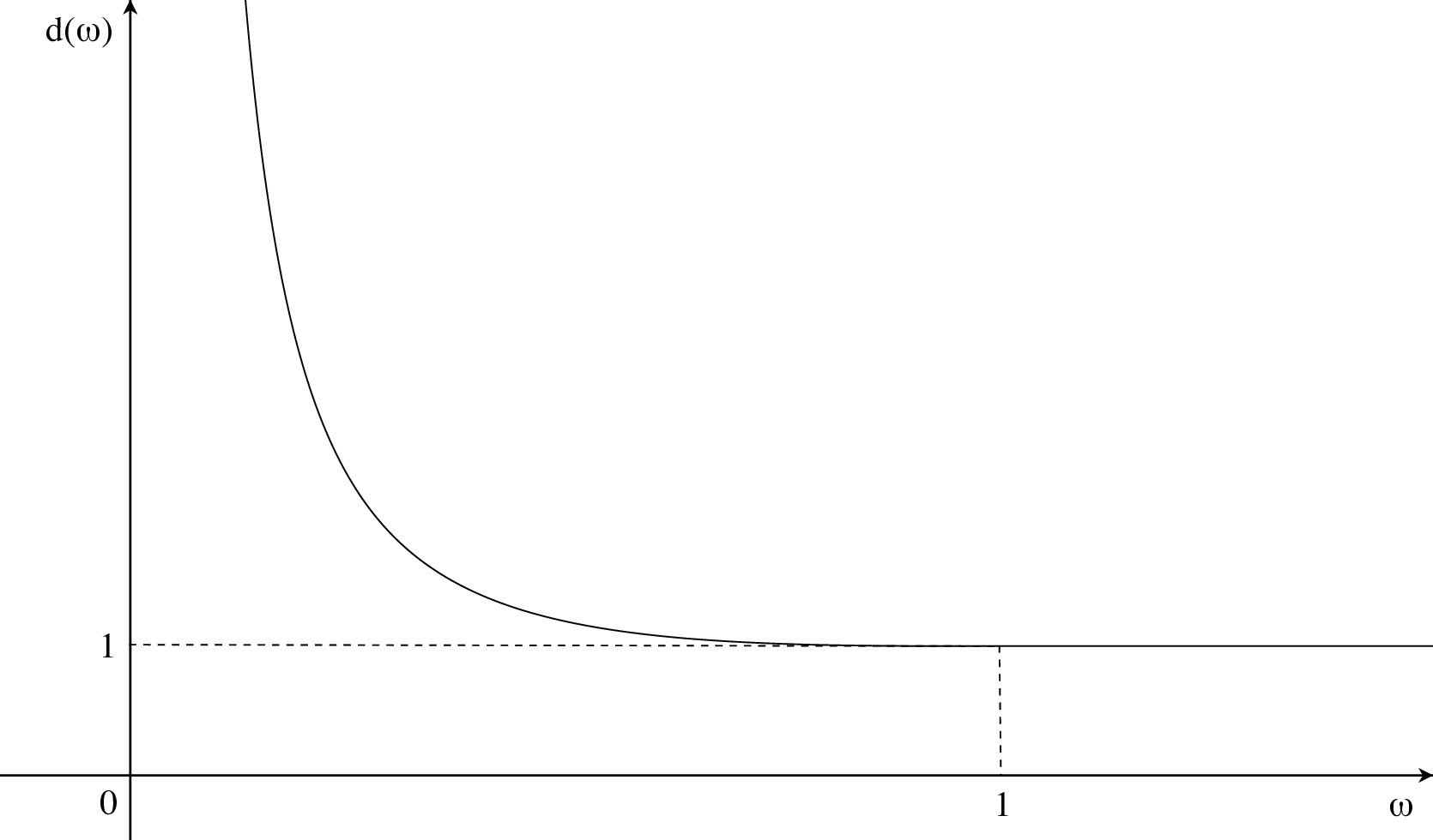
Let us consider a function d∈C∞​((0,∞))d\in\mathrm{C}^{\infty}((0,\infty)) satisfying d′​(ω)<0d^{\prime}(\omega)<0, |d′​(ω)|≤C​ω−1​d​(ω)|d^{\prime}(\omega)|\leq C\omega^{-1}d(\omega) for some positive constant CC, d⁡(ω)=1d(\omega)=1 if ω≥1\omega\geq 1, and limω→0d⁡(ω)=+∞\lim_{\omega\rightarrow 0}d(\omega)=+\infty (see Figure 1).

Refer to caption
Figure 1. The map ω↦d⁡(ω)\omega\mapsto d(\omega)

Let

𝒪τ~:=[𝟙𝒦⊗T]​𝒪τ.\tilde{\mathcal{O}_{\tau}}:=[\mathds{1}_{\mathcal{K}}\otimes T]\mathcal{O}_{\tau}. (2.10)

The following further assumptions on the interaction are made:

  • (I2)

    The following holds:

    [𝟙𝒦⊗(1+ω−1/2)ω−1d(ω)⊗𝟙L2​(Sd−1)]v~∈𝒪τ~\displaystyle\big[\mathds{1}_{\mathcal{K}}\otimes(1+\omega^{-1/2})\omega^{-1}d(\omega)\otimes\mathds{1}_{\mathrm{L}^{2}(S^{d-1})}\big]\tilde{v}\in\tilde{\mathcal{O}_{\tau}}
    [𝟙𝒦⊗(1+ω−1/2)d(ω)∂ω⊗𝟙L2​(Sd−1)]v~∈𝒪τ~,\displaystyle\big[\mathds{1}_{\mathcal{K}}\otimes(1+\omega^{-1/2})d(\omega)\partial_{\omega}\otimes\mathds{1}_{\mathrm{L}^{2}(S^{d-1})}\big]\tilde{v}\in\tilde{\mathcal{O}_{\tau}},
  • (I3)

    [𝟙𝒦⊗∂ω2⊗𝟙L2​(Sd−1)]v~∈ℬ(𝒟(K12);𝒦⊗𝔥~)\big[\mathds{1}_{\mathcal{K}}\otimes\partial^{2}_{\omega}\otimes\mathds{1}_{\mathrm{L}^{2}(S^{d-1})}\big]\tilde{v}\in\mathcal{B}(\mathcal{D}(K^{\frac{1}{2}});\mathcal{K}\otimes\tilde{\mathfrak{h}}).

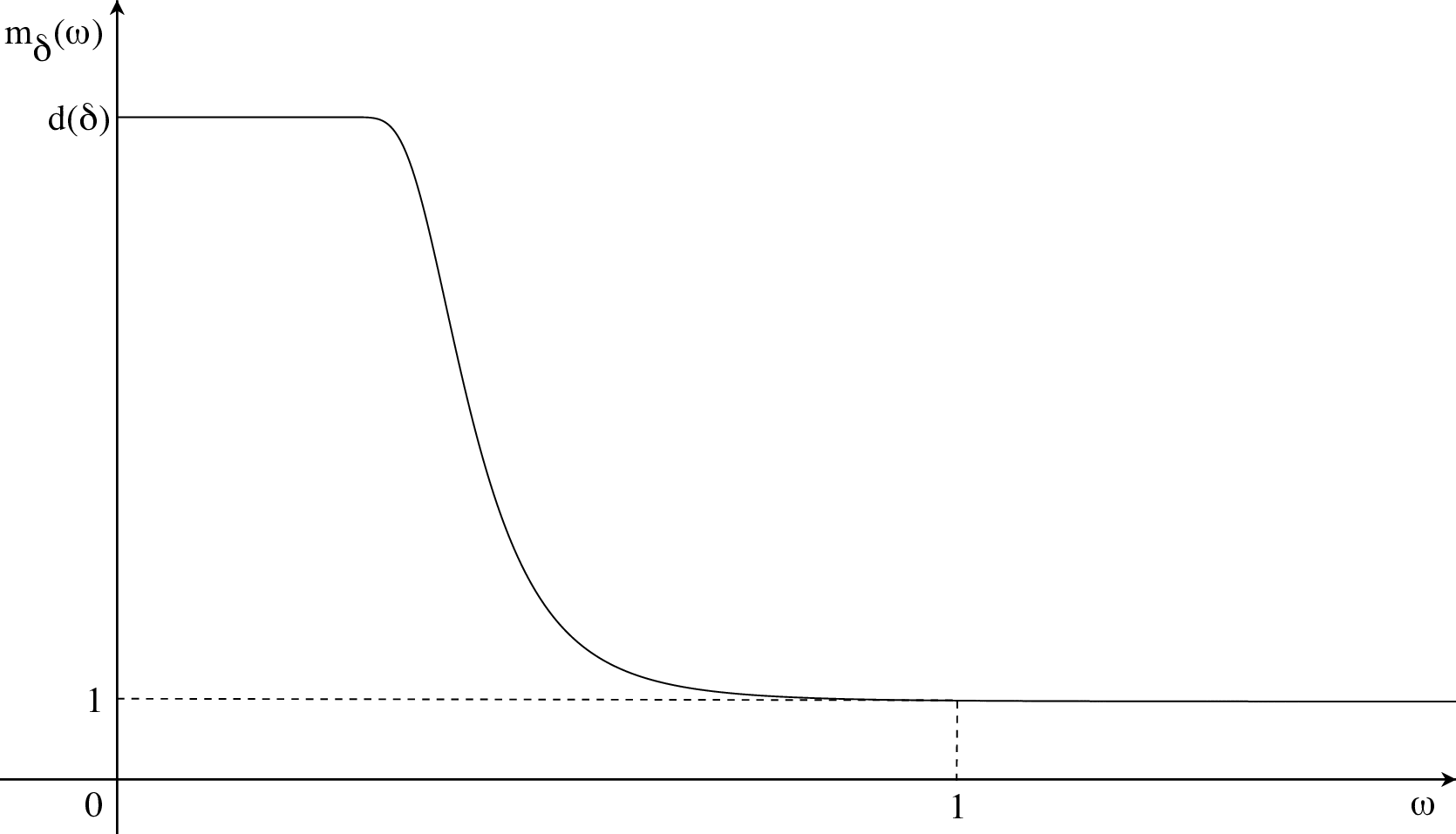
Let us recall the definition of the conjugate operator used in [GGM2]. Let χ∈C0∞​([0,∞))\chi\in\mathrm{C}_{0}^{\infty}([0,\infty)) be such that χ⁡(ω)=0\chi(\omega)=0 if ω≥1\omega\geq 1 and χ⁡(ω)=1\chi(\omega)=1 if ω≤1/2\omega\leq 1/2. For 0<δ≤1/20<\delta\leq 1/2, the function mδ∈C∞​([0,∞))m_{\delta}\in\mathrm{C}^{\infty}([0,\infty)) is defined by

mδ​(ω)=χ⁡(ωδ)​d​(δ)+(1−χ)​(ωδ)​d​(ω),m_{\delta}(\omega)=\chi(\frac{\omega}{\delta})d(\delta)+(1-\chi)(\frac{\omega}{\delta})d(\omega), (2.11)

(see Figure 2).

Refer to caption
Figure 2. The map ω↦mδ​(ω)\omega\mapsto m_{\delta}(\omega)

Consider the following operator a~δ\tilde{a}_{\delta} acting on 𝔥~\tilde{\mathfrak{h}}:

a~δ:=i​mδ​(ω)​∂∂ω+i2​d​mδd​ω​(ω),𝒟⁡(a~δ)=H01​(ℝ+)⊗L2​(Sd−1),\tilde{a}_{\delta}:={\rm i}m_{\delta}(\omega)\frac{\partial}{\partial\omega}+\frac{{\rm i}}{2}\frac{{\rm d}m_{\delta}}{{\rm d}\omega}(\omega),\quad\mathcal{D}(\tilde{a}_{\delta})=\mathrm{H}_{0}^{1}(\mathbb{R}^{+})\otimes\mathrm{L}^{2}(S^{d-1}), (2.12)

where H01​(ℝ+)H_{0}^{1}(\mathbb{R}^{+}) denotes the closure of C0∞​(ℝ+)\mathrm{C}_{0}^{\infty}(\mathbb{R}^{+}) in H1​(ℝ+)\mathrm{H}^{1}(\mathbb{R}^{+}) and C0∞​(ℝ+)\mathrm{C}_{0}^{\infty}(\mathbb{R}^{+}) is the set of smooth compactly supported functions on ℝ+\mathbb{R}^{+}. Then the operator A~δ\tilde{A}_{\delta} on ℋ~PF\tilde{\mathcal{H}}_{\mathrm{PF}} is defined by A~δ:=𝟙𝒦⊗d​Γ​(a~δ)\tilde{A}_{\delta}:=\mathds{1}_{\mathcal{K}}\otimes{\rm d}\Gamma(\tilde{a}_{\delta}). It is proved in [GGM2] that A~δ\tilde{A}_{\delta} is closed, densely defined and maximal symmetric.

Let Mδ:=𝟙𝒦⊗d​Γ​(mδ)M_{\delta}:=\mathds{1}_{\mathcal{K}}\otimes{\rm d}\Gamma(m_{\delta}) and Rδ​(v~):=−ϕ⁡(i​a~δ​v~)R_{\delta}(\tilde{v}):=-\phi({\rm i}\tilde{a}_{\delta}\tilde{v}). Then MδM_{\delta} is self-adjoint, Mδ≥0M_{\delta}\geq 0, and if vv satisfies Hypotheses (𝐈𝟏){\bf(I1)} and (𝐈𝟐){\bf(I2)}, then, by [GGM2, Lemma 6.4 OPENi)i)], Rδ​(v~)R_{\delta}(\tilde{v}) is symmetric and H~vPF\tilde{H}^{\mathrm{PF}}_{v}-bounded.

2.2. Checking the abstract assumptions

In this subsection, we verify that, on the Hilbert space ℋ=ℋ~PF\mathcal{H}=\tilde{\mathcal{H}}_{\mathrm{PF}}, the operators H=H~vPFH=\tilde{H}^{\mathrm{PF}}_{v}, M=MδM=M_{\delta}, R=Rδ​(v~)R=R_{\delta}(\tilde{v}), A=A~δA=\tilde{A}_{\delta} fulfil Conditions 1.3, 1.10 and 1.11 stated in Section 1 (provided that vv satisfies, in particular, the hypotheses stated above). The following lemma shows that Condition 1.3 (1) is satisfied.

Lemma 2.1.

Assume that vv satisfies Hypothesis (𝐈𝟏){\bf(I1)}. Then for all δ>0\delta>0,

H~vPF∈CMo1​(Mδ).\tilde{H}^{\mathrm{PF}}_{v}\in\mathrm{C}^{1}_{\mathrm{Mo}}(M_{\delta}). (2.13)
Proof.

The fact that H~vPF∈C1​(Mδ)\tilde{H}^{\mathrm{PF}}_{v}\in\mathrm{C}^{1}(M_{\delta}) follows from [GGM2, Lemma 6.4 OPENi)i)]. Moreover, since mδm_{\delta} is bounded and [ω,mδ]=0[\omega,m_{\delta}]=0, we have that [H~vPF,i​Mδ]0=−ϕ⁡(i​mδ​v~)[\tilde{H}^{\mathrm{PF}}_{v},{\rm i}M_{\delta}]^{0}=-\phi({\rm i}m_{\delta}\tilde{v}) by [GGM2, Corollary 4.13]. Using again that mδm_{\delta} is bounded, we then conclude from Hypothesis (𝐈𝟏){\bf(I1)} and [GGM2, Proposition 4.6] that [H~vPF,i​Mδ]0[\tilde{H}^{\mathrm{PF}}_{v},{\rm i}M_{\delta}]^{0} is H~0PF\tilde{H}^{\mathrm{PF}}_{0}-bounded, and hence H~vPF\tilde{H}^{\mathrm{PF}}_{v}-bounded (with relative bound 0). ∎

Lemma 2.1 together with [GGM2] imply:

Proposition 2.2.

Assume Hypothesis (𝐇𝟎){\bf(H0)} and that vv satisfies Hypotheses (𝐈𝟏){\bf(I1)}, (𝐈𝟐){\bf(I2)} and (𝐈𝟑)\bf{(I3)}. Then for all E0∈ℝE_{0}\in\mathbb{R}, there exists δ0>0\delta_{0}>0 such that for all 0<δ≤δ00<\delta\leq\delta_{0}, the operators H=H~vPFH=\tilde{H}^{\mathrm{PF}}_{v}, M=MδM=M_{\delta}, R=Rδ​(v~)R=R_{\delta}(\tilde{v}), A=A~δA=\tilde{A}_{\delta} fulfil Conditions 1.3 with I=(−∞,E0)I=(-\infty,E_{0}).

Remark 2.3.

We remark that the formulation of the Mourre estimate stated in [GGM2, Theorem 7.12] is not the same as the one considered in Condition 1.3 (2). However, one can verify that the latter is indeed a consequence of [GGM2, Theorem 7.12].

In order to verify Condition 1.10, we need to impose a further condition on vv:

  • (I4)

    The form (K⊗𝟙𝔥~)​v~−v~​K(K\otimes\mathds{1}_{\tilde{\mathfrak{h}}})\tilde{v}-\tilde{v}K extends by continuity from 𝒟⁡(K⊗𝟙Ê​𝔥~)×𝒟⁡(K)\mathcal{D}(K\otimes\mathds{1}_{\tilde{Ê\mathfrak{h}}})\times\mathcal{D}(K) to an element of 𝒪~Ê​12\tilde{\mathcal{O}}_{Ê\frac{1}{2}}.

Here 𝒪~Ê​12\tilde{\mathcal{O}}_{Ê\frac{1}{2}} is defined as 𝒪~Ê​τ\tilde{\mathcal{O}}_{Ê\tau} (see (2.4) and (2.10)). Notice that, assuming (𝐈𝟏)\bf{(I1)}, the statement above is meaningful.

We have to identify the set ℬ1,γ\mathcal{B}_{1,\gamma} used in Condition 1.10. To this end, let us first introduce some definitions. Let ℐPF​(d)\mathcal{I}_{\mathrm{PF}}(d) be defined by:

ℐPF(d):={v∈ℒ(𝒦;𝒦⊗𝔥),\displaystyle\mathcal{I}_{\mathrm{PF}}(d):=\big\{v\in\mathcal{L}(\mathcal{K};\mathcal{K}\otimes\mathfrak{h}),\, v satisfies (𝐈𝟏),(𝐈𝟐),(𝐈𝟑),(𝐈𝟒)}.\displaystyle v\text{ satisfies }\mathbf{(I1)},\mathbf{(I2)},\mathbf{(I3)},\mathbf{(I4)}\big\}. (2.14)

Observe that ℐPF​(d)\mathcal{I}_{\mathrm{PF}}(d) can be equipped with a norm, ∥⋅∥PF\|\cdot\|_{\mathrm{PF}}, matching the four conditions (𝐈𝟏)\bf{(I1)}, (𝐈𝟐)​Ê\bf{(I2)Ê}, (𝐈𝟑)\bf{(I3)}, (𝐈𝟒)\bf{(I4)} (see [FMS, Subsection 5.1]).

Let v∈ℐPF​(d)v\in\mathcal{I}_{\mathrm{PF}}(d). Let Wδ,tW_{\delta,t} denote the C0C_{0}-semigroup generated by A~δ\tilde{A}_{\delta}. We set

𝒢δPF:=𝒟⁡(|H~vPF|12)∩𝒟⁡(Mδ12).\displaystyle\mathcal{G}^{\mathrm{PF}}_{\delta}:=\mathcal{D}(|\tilde{H}^{\mathrm{PF}}_{v}|^{\frac{1}{2}})\cap\mathcal{D}(M_{\delta}^{\frac{1}{2}}). (2.15)

By Proposition 2.2, we have that H=H~vPFH=\tilde{H}^{\mathrm{PF}}_{v}, M=MδM=M_{\delta}, A=A~δA=\tilde{A}_{\delta} fulfil Condition 1.3 (3), and hence Wδ,t|𝒢δPFW_{\delta,t}|_{\mathcal{G}^{\mathrm{PF}}_{\delta}} is a C0C_{0}-semigroup. Its generator is denoted by A~𝒢δPF\tilde{A}_{\mathcal{G}^{\mathrm{PF}}_{\delta}}. Likewise, the extension of Wδ,tW_{\delta,t} to (𝒢δPF)∗(\mathcal{G}^{\mathrm{PF}}_{\delta})^{*} is a C0C_{0}-semigroup whose generator is denoted by A~(𝒢δPF)∗\tilde{A}_{(\mathcal{G}^{\mathrm{PF}}_{\delta})^{*}}.

Let 𝒱1PF\mathcal{V}_{1}^{\mathrm{PF}} denote the set of symmetric operators VV, ϵ\epsilon-bounded relatively to H~vPF\tilde{H}^{\mathrm{PF}}_{v}, such that V∈C1​(A~𝒢δPF,A~(𝒢δPF)∗)V\in\mathrm{C}^{1}(\tilde{A}_{\mathcal{G}^{\mathrm{PF}}_{\delta}};\tilde{A}_{(\mathcal{G}^{\mathrm{PF}}_{\delta})^{*}}) and [V,i​A~δ]0[V,{\rm i}\tilde{A}_{\delta}]^{0} is H~vPF\tilde{H}^{\mathrm{PF}}_{v}-bounded. It is equipped with the norm

‖V‖1PF=‖V​(H~vPF−i)−1‖+‖[V,i​A~δ]0​(H~vPF−i)−1‖.\|V\|_{1}^{\mathrm{PF}}=\|V(\tilde{H}^{\mathrm{PF}}_{v}-{\rm i})^{-1}\|+\|[V,{\rm i}\tilde{A}_{\delta}]^{0}(\tilde{H}^{\mathrm{PF}}_{v}-{\rm i})^{-1}\|. (2.16)

By [GGM2, Proposition 4.6], if ww satisfies Hypothesis (𝐈𝟏)\bf{(I1)}, then ϕ⁡(w~)\phi(\tilde{w}) is ϵ\epsilon-bounded relatively to H~vPF\tilde{H}^{\mathrm{PF}}_{v}, and, by [GGM2, Lemma 6.4 OPENi)i)], if in addition ww satisfies Hypothesis (𝐈𝟐)\bf{(I2)}, then, for any δ>0\delta>0, [ϕ⁡(w~),i​A~δ]0=−ϕ⁡(i​a~δ​w~)[\phi(\tilde{w}),{\rm i}\tilde{A}_{\delta}]^{0}=-\phi({\rm i}\tilde{a}_{\delta}\tilde{w}) is H~vPF\tilde{H}^{\mathrm{PF}}_{v}-bounded. Moreover, one can verify that the map

ℐPF​(d)∋w↦ϕ⁡(w~)∈𝒱1PF\mathcal{I}_{\mathrm{PF}}(d)\ni w\mapsto\phi(\tilde{w})\in\mathcal{V}_{1}^{\mathrm{PF}} (2.17)

is continuous (see [FMS, Lemma 5.8]).

In a separate paper, [FMS], we prove (see [FMS, Theorem 5.2]):

Proposition 2.4.

Assume Hypothesis (𝐇𝟎){\bf(H0)} and let v∈ℐPF​(d)v\in\mathcal{I}_{\mathrm{PF}}(d). For all E0∈ℝE_{0}\in\mathbb{R}, there exists δ0>0\delta_{0}>0 such that for all 0<δ≤δ00<\delta\leq\delta_{0}, the operators H=H~vPFH=\tilde{H}^{\mathrm{PF}}_{v}, M=MδM=M_{\delta}, R=Rδ​(v~)R=R_{\delta}(\tilde{v}), A=A~δA=\tilde{A}_{\delta} fulfil Condition 1.10. Here I=(−∞,E0)I=(-\infty,E_{0}) and ℬ1,γ\mathcal{B}_{1,\gamma} is given by

B1,γ={ϕ⁡(w~),w∈ℐPF​(d),‖w‖PF≤γ~},\displaystyle B_{1,\gamma}=\{\phi(\tilde{w}),w\in\mathcal{I}_{\mathrm{PF}}(d),\|w\|_{\mathrm{PF}}\leq\tilde{\gamma}\}, (2.18)

where γ~>0\tilde{\gamma}>0 is fixed sufficiently small.

Remarks 2.5.
  1.  1)

    Since the map (2.17) is continuous, for any γ>0\gamma>0, the set ℬ1,γ\mathcal{B}_{1,\gamma} is included in {V∈𝒱1PF,‖V‖1PF≤γ}\{V\in\mathcal{V}_{1}^{\mathrm{PF}},\|V\|_{1}^{\mathrm{PF}}\leq\gamma\} provided that γ~\tilde{\gamma} is chosen small enough. Moreover, B1,γB_{1,\gamma} is clearly star-shaped and symmetric with respect to 0. Hence the requirements of Condition 1.10 are satisfied.

  2.  2)

    Under the conditions of Proposition 2.4, we do not expect Condition 1.9 to be satisfied in general. Indeed, the assumption that v∈ℐPF​(d)v\in\mathcal{I}_{\mathrm{PF}}(d) in the statement of Proposition 2.4 allows us to control two commutators of H~vPF\tilde{H}^{\mathrm{PF}}_{v} with A~δ\tilde{A}_{\delta}. In order to be able to conclude that Condition 1.9 is satisfied using the method of [FMS], one would need to control three commutators of H~vPF\tilde{H}^{\mathrm{PF}}_{v} with A~δ\tilde{A}_{\delta} (see [FMS]). This would require a stronger restriction on the infrared behavior of the form factor vv than the one imposed by Hypotheses (𝐈𝟏){\bf(I1)}–(𝐈𝟐){\bf(I2)}–(𝐈𝟑){\bf(I3)}.

In order to apply Theorems 1.14 and 1.15, it remains to verify Condition 1.11. Let

𝒮=𝒟⁡(K)⊗Γfin​(C0∞​(ℝ+)⊗L2​(Sd−1)),\mathcal{S}=\mathcal{D}(K)\otimes\Gamma_{\mathrm{fin}}(\mathrm{C}_{0}^{\infty}(\mathbb{R}^{+})\otimes\mathrm{L}^{2}(S^{d-1})), (2.19)

where for ℰ⊆L2​(ℝ+)⊗L2​(Sd−1)\mathcal{E}\subseteq\mathrm{L}^{2}(\mathbb{R}^{+})\otimes\mathrm{L}^{2}(S^{d-1}),

Γfin(ℰ):={\displaystyle\Gamma_{\mathrm{fin}}(\mathcal{E}):=\big\{ Φ=(Φ(0),Φ(1),Φ(2),…)∈Γ(ℰ),∃n0,Φ(n)=0 for n≥n0}.\displaystyle\Phi=(\Phi^{(0)},\Phi^{(1)},\Phi^{(2)},\dots)\in\Gamma(\mathcal{E}),\exists n_{0},\Phi^{(n)}=0\text{ for }n\geq n_{0}\big\}. (2.20)

For any δ>0\delta>0, 𝒮\mathcal{S} is included in 𝒟⁡(H~vPF)∩𝒟⁡(Mδ)∩𝒟⁡(A~δ)\mathcal{D}(\tilde{H}^{\mathrm{PF}}_{v})\cap\mathcal{D}(M_{\delta})\cap\mathcal{D}(\tilde{A}_{\delta}). Moreover, 𝒮\mathcal{S} is a core for A~δ∗\tilde{A}_{\delta}^{*}. Therefore we get:

Proposition 2.6.

Assume that vv satisfies Hypothesis (𝐈𝟏){\bf(I1)}. Then, for all δ>0\delta>0, the operators H=H~vPFH=\tilde{H}^{\mathrm{PF}}_{v}, M=MδM=M_{\delta}, A=A~δA=\tilde{A}_{\delta} fulfil Condition 1.11.

Let us finally mention the particular case for which the unperturbed Hamiltonian under consideration is the non-interacting one, H~0PF\tilde{H}^{\mathrm{PF}}_{0}, given by

H~0PF:=K⊗𝟙Γ⁡(𝔥~)+𝟙𝒦⊗d​Γ​(ω).\tilde{H}_{0}^{\mathrm{PF}}:=K\otimes\mathds{1}_{\Gamma(\tilde{\mathfrak{h}})}+\mathds{1}_{\mathcal{K}}\otimes{\rm d}\Gamma(\omega). (2.21)

In this case, one can choose M=𝟙𝒦⊗𝒩M=\mathds{1}_{\mathcal{K}}\otimes\mathcal{N}, where 𝒩:=d​Γ​(𝟙𝔥~)\mathcal{N}:={\rm d}\Gamma(\mathds{1}_{\tilde{\mathfrak{h}}}\,) is the number operator, and A=𝟙𝒦⊗dΓ(i∂ω)A=\mathds{1}_{\mathcal{K}}\otimes{\rm d}\Gamma({\rm i}\partial_{\omega}). Then one can easily check the following proposition:

Proposition 2.7.

Assume Hypothesis (𝐇𝟎){\bf(H0)}. Then the operators H=H~0PF,M=𝟙𝒦⊗𝒩,R=0,A=𝟙𝒦⊗dΓ(i∂ω)H=\tilde{H}^{\mathrm{PF}}_{0},M=\mathds{1}_{\mathcal{K}}\otimes\mathcal{N},R=0,A=\mathds{1}_{\mathcal{K}}\otimes{\rm d}\Gamma({\rm i}\partial_{\omega}) fulfil Conditions 1.3 (with I=ℝI=\mathbb{R}) and Condition 1.9.

Remark 2.8.

The fact that Condition 1.9 is fulfilled under the conditions of Proposition 2.7 is obvious, since the unperturbed eigenstates are of the form ϕ⊗Ω\phi\otimes\Omega, where ϕ\phi is an eigenstate of KK, and Ω\Omega denotes the vacuum in Γ⁡(𝔥~)\Gamma(\tilde{\mathfrak{h}}).

2.3. Results

As a consequence of Propositions 2.2, 2.4 and 2.6, applying Theorems 1.14 and 1.15, we obtain:

Theorem 2.9.

Assume Hypothesis (𝐇𝟎){\bf(H0)}. Let v0,v∈ℐPF​(d)v_{0},v\in\mathcal{I}_{\mathrm{PF}}(d). Let JJ be a compact interval such that σpp​(Hv0PF)∩J={λ}\sigma_{\rm pp}(H^{\mathrm{PF}}_{v_{0}})\cap J=\{\lambda\}. Let Pv0P_{v_{0}} denote the eigenprojection Pv0=EHv0PF​({λ})P_{v_{0}}=E_{H^{\mathrm{PF}}_{v_{0}}}(\{\lambda\}) and P¯v0=I−Pv0\bar{P}_{v_{0}}=I-P_{v_{0}}. Then the following holds:

  • i)

    There exists σ0>0\sigma_{0}>0 such that for all 0≤|σ|≤σ00\leq|\sigma|\leq\sigma_{0}, the total multiplicity of the eigenvalues of Hv0PF+σ​ϕ​(v)H^{\mathrm{PF}}_{v_{0}}+\sigma\phi(v) in JJ is at most dimRan⁡(Pv0)\dim\mathrm{Ran}(P_{v_{0}}).

  • ii)

    Suppose in addition that

    Pv0​ϕ​(v)​Im​((Hv0PF−λ−i​0)−1​P¯v0)​ϕ​(v)​Pv0≥c​Pv0,P_{v_{0}}\phi(v){\rm Im}\,\big((H^{\mathrm{PF}}_{v_{0}}-\lambda-{\rm i}0)^{-1}\bar{P}_{v_{0}}\big)\phi(v)P_{v_{0}}\geq cP_{v_{0}}, (2.22)

    for some c>0c>0. Then there exists σ0>0\sigma_{0}>0 such that for all 0<|σ|≤σ00<|\sigma|\leq\sigma_{0},

    σpp​(Hv0PF+σ​ϕ​(v))∩J=∅.\sigma_{\rm pp}\big(H^{\mathrm{PF}}_{v_{0}}+\sigma\phi(v)\big)\cap J=\emptyset. (2.23)
Remarks 2.10.
  1.  1)

    In view of Propositions 2.2, 2.4 and 2.6, Theorems 1.14 and 1.15 imply Theorem 2.9 with H~v0PF\tilde{H}^{\mathrm{PF}}_{v_{0}} replacing Hv0PFH^{\mathrm{PF}}_{v_{0}} and ϕ⁡(v~)\phi(\tilde{v}) replacing ϕ⁡(v)\phi(v). However, using the unitary transformation mapping ℋPF\mathcal{H}_{\mathrm{PF}} to ℋ~PF\tilde{\mathcal{H}}_{\mathrm{PF}}, the statement of Theorem 2.9 clearly follows.

  2.  2)

    In the case where the unperturbed Hamiltonian is the non-interacting one, that is Hv0PF=H0PFH^{\mathrm{PF}}_{v_{0}}=H_{0}^{\mathrm{PF}} with H0PF=K⊗𝟙Γ⁡(𝔥)+𝟙𝒦⊗d​Γ​(|k|)H_{0}^{\mathrm{PF}}=K\otimes\mathds{1}_{\Gamma(\mathfrak{h})}+\mathds{1}_{\mathcal{K}}\otimes{\rm d}\Gamma(|k|), one can use Proposition 2.7 instead of Proposition 2.4 in order to conclude Theorem 2.9 ii). Indeed, it follows from [GGM2] that if vv satisfies (𝐈𝟏)\bf{(I1)}–(𝐈𝟐)\bf{(I2)}–(𝐈𝟑)\bf{(I3)}, then ϕ⁡(v~)∈𝒱2\phi(\tilde{v})\in\mathcal{V}_{2} (in the sense of Definition 1.6). Hence, since Condition 1.9 is satisfied by Proposition 2.7, we can apply Theorem 1.15 with Condition OPENi)\ref{item:a}) instead of Condition OPENii)\ref{item:b}). For a general v0∈ℐPF​(d)v_{0}\in\mathcal{I}_{\mathrm{PF}}(d), however, we have to apply Theorem 1.15 with Condition OPENi)\ref{item:a}) (see Remark 2.5 2) above).

The latter result (the absence of eigenvalues of H0PF+σ​ϕ​(v)H^{\mathrm{PF}}_{0}+\sigma\phi(v) for sufficiently small σ≠0\sigma\neq 0 according to Fermi Golden Rule) already appears in [DJ] assuming in particular that ⟨∂ω⟩νv~∈ℬ(𝒦;𝒦⊗𝔥~)\langle\partial_{\omega}\rangle^{\nu}\tilde{v}\in\mathcal{B}(\mathcal{K};\mathcal{K}\otimes\tilde{\mathfrak{h}}) for some ν>1\nu>1. Let us also mention [Go] where a similar result with different assumptions on the form factor is obtained, still for sufficiently small values of the coupling constant. Besides, in [DJ], upper semicontinuity of the point spectrum of H0PF+σ​ϕ​(v)H^{\mathrm{PF}}_{0}+\sigma\phi(v) (in the sense stated in Theorem 2.9 i)) is obtained for sufficiently small σ\sigma, assuming that ⟨∂ω⟩νv~∈ℬ(𝒦;𝒦⊗𝔥~)\langle\partial_{\omega}\rangle^{\nu}\tilde{v}\in\mathcal{B}(\mathcal{K};\mathcal{K}\otimes\tilde{\mathfrak{h}}) for some ν>2\nu>2. The main achievement of our paper, as far as massless Pauli-Fierz models are concerned, is to provide a method which allows us to consider Hv0PFH^{\mathrm{PF}}_{v_{0}} as the unperturbed Hamiltonian, for any v0v_{0} belonging to ℐPF​(d)\mathcal{I}_{\mathrm{PF}}(d).

A model sharing several properties with the one considered in this subsection is the so-called “standard model of non-relativistic QED”. For results on spectral theory in this context involving the Mourre method, we refer to [Sk, BFS, BFSS, DJ, FGS].

2.4. Example: The massless Nelson model

An example of a model satisfying the hypotheses of Subsection 2.1 is the Nelson model of confined non-relativistic quantum particles interacting with massless scalar bosons. The Hilbert space is given by

ℋN:=L2​(ℝ3​P)⊗ℱ,\mathcal{H}_{\mathrm{N}}:=\mathrm{L}^{2}(\mathbb{R}^{3P})\otimes\mathcal{F}, (2.24)

where ℱ:=Γ⁡(L2​(ℝ3))\mathcal{F}:=\Gamma(\mathrm{L}^{2}(\mathbb{R}^{3})) is the symmetric Fock space over L2​(ℝ3)\mathrm{L}^{2}(\mathbb{R}^{3}) (see (2.1)). The Nelson Hamiltonian acts on ℋN\mathcal{H}_{\mathrm{N}} and is defined by

HρN:=K⊗𝟙ℱ+𝟙L2​(ℝ3​P)⊗d​Γ​(|k|)+Iρ​(x).H^{\mathrm{N}}_{\rho}:=K\otimes\mathds{1}_{\mathcal{F}}+\mathds{1}_{\mathrm{L}^{2}(\mathbb{R}^{3P})}\otimes{\rm d}\Gamma(|k|)+I_{\rho}(x). (2.25)

Here x=(x1,…,xP)x=(x_{1},\dots,x_{P}), and KK is a Schrödinger operator on L2​(ℝ3​P)\mathrm{L}^{2}(\mathbb{R}^{3P}) describing the dynamics of PP non-relativistic particles. We suppose that KK is given by

K:=∑i=1P12​mi​Δi+∑i<jVi​j​(xi−xj)+W⁡(x1,…,xp),K:=\sum_{i=1}^{P}\frac{1}{2m_{i}}\Delta_{i}+\sum_{i<j}V_{ij}(x_{i}-x_{j})+W(x_{1},\dots,x_{p}), (2.26)

where the masses mim_{i} are positive, the confining potential WW satisfies

  • (W0)

    W∈Lloc2​(ℝ3​P)W\in\mathrm{L}^{2}_{\mathrm{loc}}(\mathbb{R}^{3P}) and there exist positive constants c0,c1>0c_{0},c_{1}>0 and α>2\alpha>2 such that W⁡(x)≥c0​|x|2​α−c1W(x)\geq c_{0}|x|^{2\alpha}-c_{1},

and the pair potentials Vi​jV_{ij} satisfy

  • (V0)

    The Vi​jV_{ij}’s are Δ\Delta-bounded with relative bound 0.

Without loss of generality, we can assume that K≥0K\geq 0. Note that (𝐖𝟎){\bf(W0)} implies that Hypothesis (𝐇𝟎){\bf(H0)} of Subsection 2.1 is satisfied.

The coupling Iρ​(x)I_{\rho}(x) in (2.25) is of the form

Iρ​(x):=∑i=1PΦρ​(xi),I_{\rho}(x):=\sum_{i=1}^{P}\Phi_{\rho}(x_{i}), (2.27)

where, for y∈ℝ3y\in\mathbb{R}^{3}, Φρ​(y)\Phi_{\rho}(y) is the field operator defined by

Φρ(y):=12∫ℝ3(ρ(k)e−ik⋅ya∗(k)+ρ¯(k)ei​k⋅xa(k))dk.\Phi_{\rho}(y):=\frac{1}{\sqrt{2}}\int_{\mathbb{R}^{3}}\big(\rho(k)e^{-{\rm i}k\cdot y}a^{*}(k)+\bar{\rho}(k)e^{{\rm i}k\cdot x}a(k)\big){\rm d}k. (2.28)

In particular, Iρ​(x)I_{\rho}(x) can be written under the form Iρ​(x)=ϕ⁡(ΨN​(ρ))I_{\rho}(x)=\phi(\Psi_{\mathrm{N}}(\rho)), where

ΨN​(ρ)∈ℬ⁡(L2​(ℝ3​P),L2​(ℝ3​P)⊗L2​(ℝ3))=ℬ⁡(L2​(ℝ3​P),L2​(ℝ3,L2​(ℝ3​P)))\Psi_{\mathrm{N}}(\rho)\in\mathcal{B}(\mathrm{L}^{2}(\mathbb{R}^{3P});\mathrm{L}^{2}(\mathbb{R}^{3P})\otimes\mathrm{L}^{2}(\mathbb{R}^{3}))=\mathcal{B}(\mathrm{L}^{2}(\mathbb{R}^{3P});\mathrm{L}^{2}(\mathbb{R}^{3};\mathrm{L}^{2}(\mathbb{R}^{3P})))

is defined by

(ΨN(ρ)ψ)(k)(x1,…,xP)=∑j=1Pe−ik⋅xjρ(k)ψ(x1,…,xP).(\Psi_{\mathrm{N}}(\rho)\psi)(k)(x_{1},\dots,x_{P})=\sum_{j=1}^{P}e^{-{\rm i}k\cdot x_{j}}\rho(k)\psi(x_{1},\dots,x_{P}). (2.29)

Hence HρNH^{\mathrm{N}}_{\rho} is a Pauli-Fierz Hamiltonian in the sense of Subsection 2.1, with 𝒦=L2​(ℝ3​P)\mathcal{K}=\mathrm{L}^{2}(\mathbb{R}^{3P}) and 𝔥=L2​(ℝ3)\mathfrak{h}=\mathrm{L}^{2}(\mathbb{R}^{3}).

For simplicity, we assume that ρ\rho only depends on kk through its norm, |k||k|, and, going to polar coordinates, we introduce

ρ~​(ω)=ω​ρ​(ω,0,0),ω∈ℝ+.\tilde{\rho}(\omega)=\omega\rho(\omega,0,0),\quad\omega\in\mathbb{R}^{+}. (2.30)

Our set of conditions on ρ~\tilde{\rho} is the following:

  • (ρ\rho1)

    ∫0∞(1+ω−1)​|ρ~​(ω)|2​𝑑ω<∞\int_{0}^{\infty}(1+\omega^{-1})|\tilde{\rho}(\omega)|^{2}{\rm d}\omega<\infty,

  • (ρ\rho2)

    ∫0∞(1+ω−1)​d​(ω)2​[ω−2​|ρ~​(ω)|2+|d​ρ~d​ω​(ω)|2]​𝑑ω<∞\int_{0}^{\infty}(1+\omega^{-1})d(\omega)^{2}\big[\omega^{-2}|\tilde{\rho}(\omega)|^{2}+\big|\frac{{\rm d}\tilde{\rho}}{{\rm d}\omega}(\omega)\big|^{2}\big]{\rm d}\omega<\infty,

  • (ρ\rho3)

    ∫0∞|d2​ρ~d​ω2​(ω)|2​𝑑ω<∞\int_{0}^{\infty}\big|\frac{{\rm d}^{2}\tilde{\rho}}{{\rm d}\omega^{2}}(\omega)\big|^{2}{\rm d}\omega<\infty,

  • (ρ\rho4)

    ∫0∞ω4​|ρ~​(ω)|2​𝑑ω<∞\int_{0}^{\infty}\omega^{4}\big|\tilde{\rho}(\omega)\big|^{2}{\rm d}\omega<\infty,

where dd denotes the function considered in Subsection 2.1. Note that (ρ\rho1)–(ρ\rho2)–(ρ\rho3) are the assumptions made in [GGM2]. The further assumption (ρ\rho4) is made in order that Hypothesis (I4) of Subsection 2.2 is satisfied. We observe that (ρ\rho2) and (ρ\rho4) imply (ρ\rho1).

The set of functions ρ\rho satisfying (ρ\rho1)–(ρ\rho2)–(ρ\rho3)–(ρ\rho4) is denoted by ℐN​(d)\mathcal{I}_{\mathrm{N}}(d). The following proposition is proven in [FMS, Subsection 5.2]:

Proposition 2.11.

Let ρ∈ℐN​(d)\rho\in\mathcal{I}_{\mathrm{N}}(d). Then ΨN​(ρ)\Psi_{\mathrm{N}}(\rho) defined as in (2.29) belongs to ℐPF​Ê​(d)\mathcal{I}_{\mathrm{PF}Ê}(d).

An example of ρ\rho, and hence ρ~\tilde{\rho}, satisfying (ρ\rho1)–(ρ\rho2)–(ρ\rho3)–(ρ\rho4) is

ρ⁡(k)=e−|k|22​Λ2​|k|−12+ϵ,ρ~​(ω)=e−ω22​Λ2​ω12+ϵ,\rho(k)=e^{-\frac{|k|^{2}}{2\Lambda^{2}}}|k|^{-\frac{1}{2}+\epsilon},\quad\tilde{\rho}(\omega)=e^{-\frac{\omega^{2}}{2\Lambda^{2}}}\omega^{\frac{1}{2}+\epsilon}, (2.31)

with 0<Λ<∞0<\Lambda<\infty and ϵ>1\epsilon>1.

From Proposition 2.11 and Theorem 2.9, we obtain:

Theorem 2.12.

Assume that Hypotheses (𝐖𝟎){\bf(W0)} and (𝐕𝟎){\bf(V0)} hold. Let ρ0,ρ∈ℐN​(d)\rho_{0},\rho\in\mathcal{I}_{\mathrm{N}}(d). Let JJ be a compact interval such that σpp​(Hρ0N)∩J={λ}\sigma_{\rm pp}(H^{\mathrm{N}}_{\rho_{0}})\cap J=\{\lambda\}. Let Pρ0P_{\rho_{0}} denote the eigenprojection Pρ0=EHρ0N​({λ})P_{\rho_{0}}=E_{H^{\mathrm{N}}_{\rho_{0}}}(\{\lambda\}) and P¯ρ0=I−Pρ0\bar{P}_{\rho_{0}}=I-P_{\rho_{0}}. Then the following holds:

  • i)

    There exists σ0>0\sigma_{0}>0 such that for all 0≤|σ|≤σ00\leq|\sigma|\leq\sigma_{0}, the total multiplicity of the eigenvalues of Hρ0N+σ​Iρ​(x)H^{\mathrm{N}}_{\rho_{0}}+\sigma I_{\rho}(x) in JJ is at most dimRan⁡(Pρ0)\dim\mathrm{Ran}(P_{\rho_{0}}).

  • ii)

    Suppose in addition that

    Pρ0​Iρ​(x)​Im​((Hρ0N−λ−i​0)−1​P¯ρ0)​Iρ​(x)​Pρ0≥c​Pρ0,P_{\rho_{0}}I_{\rho}(x){\rm Im}\,\big((H^{\mathrm{N}}_{\rho_{0}}-\lambda-{\rm i}0)^{-1}\bar{P}_{\rho_{0}}\big)I_{\rho}(x)P_{\rho_{0}}\geq cP_{\rho_{0}}, (2.32)

    for some c>0c>0. Then there exists σ0>0\sigma_{0}>0 such that for all 0<|σ|≤σ00<|\sigma|\leq\sigma_{0},

    σpp​(Hρ0N+σ​Iρ​(x))∩J=∅.\sigma_{\rm pp}\big(H^{\mathrm{N}}_{\rho_{0}}+\sigma I_{\rho}(x)\big)\cap J=\emptyset. (2.33)

In fact, the confinement assumption (𝐖𝟎){\bf(W0)} allows one to make use of a unitary dressing transformation (see e.g. [GGM2, FMS]) in order to “improve” the infrared behavior of the form factor in the Hamiltonian Hρ0NH^{\mathrm{N}}_{\rho_{0}}. More precisely, let (ρ\rho1’) denote the following condition:

  • (ρ\rho1’)

    ∫0∞(1+ω−2)​|ρ~​(ω)|2​𝑑ω<∞\int_{0}^{\infty}(1+\omega^{-2})|\tilde{\rho}(\omega)|^{2}{\rm d}\omega<\infty.

Assuming that ρ0\rho_{0} satisfies this condition, the unitary operator

Uρ0:=e−iPΦiρ0/|⋅|U_{\rho_{0}}:=e^{-{\rm i}P\Phi_{{\rm i}\rho_{0}/|\cdot|}} (2.34)

is well-defined and we can consider the Hamiltonian

Hρ0N′:=\displaystyle H_{\rho_{0}}^{\mathrm{N}^{\prime}}:= (𝟙𝒦⊗Uρ0)​HÊ​ρ0N​(𝟙𝒦⊗Uρ0∗)\displaystyle(\mathds{1}_{\mathcal{K}}\otimes U_{\rho_{0}})H_{Ê\rho_{0}}^{\mathrm{N}}(\mathds{1}_{\mathcal{K}}\otimes U_{\rho_{0}}^{*})
=\displaystyle= KÊ​ρ0⊗𝟙ℱ+𝟙Ê​𝒦⊗d​Γ​(|k|)+IÊ​ρ0​(x)−IÊ​ρ0​(0),\displaystyle K_{Ê\rho_{0}}\otimes\mathds{1}_{\mathcal{F}}+\mathds{1}_{Ê\mathcal{K}}\otimes{\rm d}\Gamma(|k|)+I_{Ê\rho_{0}}(x)-I_{Ê\rho_{0}}(0), (2.35)

where

Kρ0:=\displaystyle K_{\rho_{0}}:= K+P2Ê​2​∫Ê​ℝ3|ρ0​(k)|2|k|​𝑑k−P​∑j=1P∫Ê​ℝ3|ρ0​(k)|2|k|​cos​(k⋅xj)​𝑑k.\displaystyle K+\frac{P^{2}}{Ê2}\int_{Ê\mathbb{R}^{3}}\frac{|\rho_{0}(k)|^{2}}{|k|}{\rm d}k-P\sum_{j=1}^{P}\int_{Ê\mathbb{R}^{3}}\frac{|\rho_{0}(k)|^{2}}{|k|}\mathrm{cos}(k\cdot x_{j}){\rm d}k. (2.36)

In the same way as in (2.29), we observe that Iρ0​(x)−Iρ0​(0)=ϕ⁡(ΨN′​(ρ0))I_{\rho_{0}}(x)-I_{\rho_{0}}(0)=\phi(\Psi^{\prime}_{\mathrm{N}}(\rho_{0})), where ΨN′​(ρ0)\Psi^{\prime}_{\mathrm{N}}(\rho_{0}) is defined by

(ΨN′(ρ0)ψ)(k)(x1,…,xP)=∑j=1P(e−ik⋅xj−1)ρ0(k)ψ(x1,…,xP).(\Psi^{\prime}_{\mathrm{N}}(\rho_{0})\psi)(k)(x_{1},\dots,x_{P})=\sum_{j=1}^{P}(e^{-{\rm i}k\cdot x_{j}}-1)\rho_{0}(k)\psi(x_{1},\dots,x_{P}). (2.37)

In particular, Hρ0N′H_{\rho_{0}}^{\mathrm{N}^{\prime}} is a Pauli-Fierz Hamiltonian in the sense of Subsection 2.1.

We consider the following further conditions:

  • (ρ\rho2’)

    ∫0∞|d​ρ~d​ω​(ω)|2​𝑑ω<∞\int_{0}^{\infty}\big|\frac{{\rm d}\tilde{\rho}}{{\rm d}\omega}(\omega)\big|^{2}{\rm d}\omega<\infty,

  • (ρ\rho3’)

    ∫0∞(1+ω2)−1​ω2​|d2​ρ~d​ω2​(ω)|2​𝑑ω<∞\int_{0}^{\infty}(1+\omega^{2})^{-1}\omega^{2}\big|\frac{{\rm d}^{2}\tilde{\rho}}{{\rm d}\omega^{2}}(\omega)\big|^{2}{\rm d}\omega<\infty,

and we denote by ℐN′​(d)\mathcal{I}_{\mathrm{N}}^{\prime}(d) the set of functions ρ\rho satisfying (ρ\rho1’)–(ρ\rho2’)–(ρ\rho3’)–(ρ\rho4). In [FMS, Subsection 5.2], we verify that if ρ0∈ℐN′​(d)\rho_{0}\in\mathcal{I}_{\mathrm{N}}^{\prime}(d), then ΨN′​(ρ0)\Psi^{\prime}_{\mathrm{N}}(\rho_{0}) defined as in (2.37) belongs to ℐPF​Ê​(d)\mathcal{I}_{\mathrm{PF}Ê}(d). Notice that for any 0<Λ<∞0<\Lambda<\infty and ϵ>0\epsilon>0, the function given in (2.31) belongs to ℐN′​(d)\mathcal{I}_{\mathrm{N}}^{\prime}(d).

As in the statement of Theorem 2.12, we consider a perturbation of the Hamiltonian Hρ0NH_{\rho_{0}}^{\mathrm{N}} of the form σ​Iρ​(x)\sigma I_{\rho}(x). After the dressing transformation, the perturbation becomes

σ​Iρ0,ρ​(x):=\displaystyle\sigma I_{\rho_{0},\rho}(x):= σ⁡(𝟙𝒦⊗Uρ0)​Iρ​(x)​(𝟙𝒦⊗Uρ0∗)\displaystyle\sigma(\mathds{1}_{\mathcal{K}}\otimes U_{\rho_{0}})I_{\rho}(x)(\mathds{1}_{\mathcal{K}}\otimes U_{\rho_{0}}^{*})
=\displaystyle= Iρ(x)−P∑j=1PRe∫ℝ3ρ¯0​(k)​ρ​(k)|k|e−ik⋅xjdk.\displaystyle I_{\rho}(x)-P\sum_{j=1}^{P}\mathrm{Re}\int_{\mathbb{R}^{3}}\frac{\bar{\rho}_{0}(k)\rho(k)}{|k|}e^{-{\rm i}k\cdot x_{j}}{\rm d}k. (2.38)

Notice that σ​Iρ0,ρ​(x)\sigma I_{\rho_{0},\rho}(x) is not a field operator in the sense of Subsection 2.1. Hence it does not belong to the class of perturbations considered in Theorem 2.9. Nevertheless, proceeding in the same way as what we did in Subsection 2.2 to deduce Theorem 2.9 (see in particular [FMS, Theorem 1.2 2)] for the verification of Condition 1.10 in the present context), we obtain:

Theorem 2.13.

Assume that Hypotheses (𝐖𝟎){\bf(W0)} and (𝐕𝟎){\bf(V0)} are satisfied and let ρ0∈ℐN′​(d)\rho_{0}\in\mathcal{I}_{\mathrm{N}}^{\prime}(d) and ρ∈ℐN​(d)\rho\in\mathcal{I}_{\mathrm{N}}(d). Let JJ be a compact interval such that σpp​(Hρ0N)∩J={λ}\sigma_{\rm pp}(H^{\mathrm{N}}_{\rho_{0}})\cap J=\{\lambda\}. Let Pρ0P_{\rho_{0}} denote the eigenprojection Pρ0=EHρ0N​({λ})P_{\rho_{0}}=E_{H^{\mathrm{N}}_{\rho_{0}}}(\{\lambda\}) and P¯ρ0=I−Pρ0\bar{P}_{\rho_{0}}=I-P_{\rho_{0}}. Then the conclusions 𝑂𝑃𝐸𝑁i)\mathrm{i)} and 𝑂𝑃𝐸𝑁ii)\mathrm{ii)} of Theorem 2.12 hold.

Observe that, thanks to the unitary dressing transformation Uρ0U_{\rho_{0}}, the Fermi golden rule condition (2.32) is equivalent to the following one:

Pρ0′​Iρ0,ρ​(x)​Im​((Hρ0N′−λ−i​0)−1​P¯ρ0′)​Iρ0,ρ​(x)​Pρ0′≥c​Pρ0′,P_{\rho_{0}}^{\prime}I_{\rho_{0},\rho}(x){\rm Im}\,\big((H^{\mathrm{N}^{\prime}}_{\rho_{0}}-\lambda-{\rm i}0)^{-1}\bar{P}_{\rho_{0}}^{\prime}\big)I_{\rho_{0},\rho}(x)P_{\rho_{0}}^{\prime}\geq cP_{\rho_{0}}^{\prime}, (2.39)

where

Pρ0′:=EHρ0N′​({λ}).P_{\rho_{0}}^{\prime}:=E_{H^{\mathrm{N}^{\prime}}_{\rho_{0}}}(\{\lambda\}). (2.40)

Hence the conclusions of Theorem 2.13 for Hρ0NH_{\rho_{0}}^{\mathrm{N}} follows from the corresponding statements for Hρ0N′H_{\rho_{0}}^{\mathrm{N}^{\prime}}.

In Theorem 2.13, ρ0\rho_{0} and ρ\rho do not belong to the same class of form factors (as far as the infrared singularity is concerned, ρ0\rho_{0} is allowed to have a more singular infrared behavior than ρ\rho). This is due to the fact that the unitary transformation Uρ0U_{\rho_{0}} is ρ0\rho_{0}-dependent, so that the Hamiltonian obtained after the transformation, Hρ0N′H^{\mathrm{N}^{\prime}}_{\rho_{0}}, does not depend linearly on ρ0\rho_{0}. Thus, a perturbation of the form Hρ0+σ​ρN′−Hρ0N′H^{\mathrm{N}^{\prime}}_{\rho_{0}+\sigma\rho}-H^{\mathrm{N}^{\prime}}_{\rho_{0}} does not belong to the class of linear perturbations considered in this paper (at least as far as the Fermi Golden Rule criterion is concerned). Nevertheless, since the non-linear terms in σ\sigma in the expression of Hρ0+σ​ρN′−Hρ0N′H^{\mathrm{N}^{\prime}}_{\rho_{0}+\sigma\rho}-H^{\mathrm{N}^{\prime}}_{\rho_{0}} act only on the particle Hilbert space L2​(ℝ3​P)\mathrm{L}^{2}(\mathbb{R}^{3P}) (and hence, in particular, commute with the conjugate operator A~δ\tilde{A}_{\delta} of Subsection 2.1), we expect that the method of this paper can be extended to cover the case where both ρ0\rho_{0} and ρ\rho belong to ℐN′​(d)\mathcal{I}_{\mathrm{N}}^{\prime}(d).

3. Reduced Limiting Absorption Principle at an eigenvalue

In this section we prove two different “reduced Limiting Absorption Principles”. Assuming Conditions 1.3 and 1.7, we shall prove a Limiting Absorption Principle for the reduced unperturbed Hamiltonian H​P¯H\bar{P} (where P=EH​({λ})P=E_{H}(\{\lambda\}) and P¯=I−P\bar{P}=I-P). If the stronger Condition 1.9 is satisfied, we shall obtain a Limiting Absorption Principle for the reduced perturbed Hamiltonian H+α​P+σ​VH+\alpha P+\sigma V (for some α>0\alpha>0), provided that V∈𝒱2V\in\mathcal{V}_{2} and that σ\sigma is sufficiently small.

Let us first recall from [GGM1]:

Theorem 3.1.

Assume that Conditions 1.3 hold. Suppose J⊆IJ\subseteq I is a compact interval such that σpp​(H)∩J=∅\sigma_{\rm pp}(H)\cap J=\emptyset. Let S={z∈ℂ,Rez∈J,0<|Imz|≤1}S=\{z\in\mathbb{C},{\rm Re}\,z\in J,0<|{\rm Im}\,z|\leq 1\}. For any 1/2<s≤11/2<s\leq 1,

supz∈S‖⟨A⟩−s​(H−z)−1​⟨A⟩−s‖<∞.\sup_{z\in S}\|\langle A\rangle^{-s}(H-z)^{-1}\langle A\rangle^{-s}\|<\infty. (3.1)

Moreover the function S∋z→⟨A⟩−s​(H−z)−1​⟨A⟩−s∈ℬ⁡(ℋ)S\ni z\to\langle A\rangle^{-s}(H-z)^{-1}\langle A\rangle^{-s}\in\mathcal{B}(\mathcal{H}) is uniformly Hölder continuous of order s−1/2s-1/2.

Remarks 3.2.
  1.  1)

    Strictly speaking, the Mourre estimate formulated in Condition 1.3 (2) together with [GGM1] yield that, for any η∈J\eta\in J, there is a neighbourhood IηI_{\eta} such that, for any compact interval Jη⊆IηJ_{\eta}\subseteq I_{\eta}, the Limiting Absorption Principle (3.1) holds with JηJ_{\eta} replacing JJ. The statement of Theorem 3.1 then follows from the compactness of JJ and a covering argument (see Step II in the proof of Theorem 3.4 below for the use of the same argument).

  2.  2)

    The result [GGM1, Theorem 3.3] is stronger in that the bound (3.1) holds in a stronger operator topology (given in terms of the Hilbert spaces 𝒢\mathcal{G} and OPEN𝒢∗)\mathcal{G}^{*}). For our purposes (3.1) suffices. A similar remark is due for the bounds (3.2) and (3.21) given below.

We shall now obtain a result similar to Theorem 3.1 for a reduced resolvent.

Theorem 3.3.

Assume that Conditions 1.3 and Condition 1.7 hold. Suppose J⊆IJ\subseteq I is a compact interval such that σpp​(H)∩J={λ}\sigma_{\rm pp}(H)\cap J=\{\lambda\}. Let PP denote the eigenprojection P=EH​({λ})P=E_{H}(\{\lambda\}) and let P¯=I−P\bar{P}=I-P. Let S={z∈ℂ,Rez∈J,0<|Imz|≤1}S=\{z\in\mathbb{C},{\rm Re}\,z\in J,0<|{\rm Im}\,z|\leq 1\}. For any 1/2<s≤11/2<s\leq 1,

supz∈S‖⟨A⟩−s​(H−z)−1​P¯​⟨A⟩−s‖<∞.\sup_{z\in S}\|\langle A\rangle^{-s}(H-z)^{-1}\bar{P}\langle A\rangle^{-s}\|<\infty. (3.2)

Moreover there exists C>0C>0 such that for all z,z′∈Sz,z^{\prime}\in S,

‖⟨A⟩−s​((H−z)−1−(H−z′)−1)​P¯​⟨A⟩−s‖≤C​|z−z′|s−12.\begin{split}&\left\|\langle A\rangle^{-s}\left((H-z)^{-1}-(H-z^{\prime})^{-1}\right)\bar{P}\langle A\rangle^{-s}\right\|\leq C|z-z^{\prime}|^{s-\frac{1}{2}}.\end{split} (3.3)
Proof.

It follows from Conditions 1.3 and Condition 1.7 that σpp​(H)\sigma_{\mathrm{pp}}(H) is finite in a neighbourhood of λ\lambda. Hence, possibly by considering a bigger compact interval, we can assume without loss of generality that λ\lambda is included in the interior of JJ.

Consider Condition 1.3 (2) with η=λ\eta=\lambda. Let Jλ⊆JJ_{\lambda}\subseteq J be a compact neighbourhood of λ\lambda such that fλ=1f_{\lambda}=1 on a neighbourhood of JλJ_{\lambda}. Applying Theorem 3.1 on [infJ,infJλ][\inf J,\inf J_{\lambda}] and using that P+P¯=IP+\bar{P}=I, we obtain that

supz∈ℂ,Re​z∈[infJ,infJλ],0<|Im​z|≤1‖⟨A⟩−s​(H−z)−1​P¯​⟨A⟩−s‖<∞,\sup_{z\in\mathbb{C},{\rm Re}\,z\in[\inf J,\inf J_{\lambda}],0<|{\rm Im}\,z|\leq 1}\|\langle A\rangle^{-s}(H-z)^{-1}\bar{P}\langle A\rangle^{-s}\|<\infty, (3.4)

and that z↦⟨A⟩−s​(H−z)−1​P¯​⟨A⟩−sz\mapsto\langle A\rangle^{-s}(H-z)^{-1}\bar{P}\langle A\rangle^{-s} is Hölder continuous of order s−1/2s-1/2 on {z∈ℂ,Rez∈[infJ,infJλ],0<|Imz|≤1}\{z\in\mathbb{C},{\rm Re}\,z\in[\inf J,\inf J_{\lambda}],0<|{\rm Im}\,z|\leq 1\}. The same holds with [supJλ,supJ][\sup J_{\lambda},\sup J] replacing [infJ,infJλ][\inf J,\inf J_{\lambda}]. Therefore, to conclude the proof, one can verify that it is sufficient to establish the statement of Theorem 3.3 with JJ replaced by JλJ_{\lambda}. We can follow the proof of [GGM1, Theorem 3.3]. We emphasize the differences with [GGM1] and refer the reader to that paper for more details.

We obtain from (1.4) with η=λ\eta=\lambda that

M+R≥2−1​c0​I−C2​fλ⊥​(H)2​⟨H⟩−fλ​(H)​K​fλ​(H).M+R\geq 2^{-1}c_{0}I-C_{2}f^{\bot}_{\lambda}(H)^{2}\langle H\rangle-f_{\lambda}(H)Kf_{\lambda}(H). (3.5)

Since fλ​(H)f_{\lambda}(H) goes strongly to PP as λ→0\lambda\to 0, we obtain

M+R≥3−1​c0​I−C2​fλ⊥​(H)2​⟨H⟩−C3​P,M+R\geq 3^{-1}c_{0}I-C_{2}f^{\bot}_{\lambda}(H)^{2}\langle H\rangle-C_{3}P, (3.6)

which is valid if the support of fλf_{\lambda} is sufficiently close to λ\lambda. Applying P¯\bar{P} from the left and from the right in (3.6) yields

P¯​(M+R)​P¯≥3−1​c0​P¯−C2​P¯​fλ⊥​(H)2​⟨H⟩​P¯.\bar{P}(M+R)\bar{P}\geq 3^{-1}c_{0}\bar{P}-C_{2}\bar{P}f^{\bot}_{\lambda}(H)^{2}\langle H\rangle\bar{P}. (3.7)

Next, we can mimic the proof of [GGM1, Theorem 3.3] using (3.7) and the following slightly different constructions: In Subsection 3.4 of [GGM1] the operator HϵH_{\epsilon} (related to the one from the seminal paper [Mo]) is taken as Hϵ=H−i​ϵ​H′H_{\epsilon}=H-{\rm i}\epsilon H^{\prime}. Notice that here and henceforth we can assume without loss that H′H^{\prime} is closed (possibly by taking the closure).

We propose to take

H¯ϵ:=H−i​ϵ​P¯​H′​P¯,\bar{H}_{\epsilon}:=H-{\rm i}\epsilon\bar{P}H^{\prime}\bar{P}, (3.8)

with domain 𝒟⁡(H¯ϵ):=𝒟⁡(H)∩𝒟⁡(M)∩Ran⁡(P¯)\mathcal{D}(\bar{H}_{\epsilon}):=\mathcal{D}(H)\cap\mathcal{D}(M)\cap\mathrm{Ran}(\bar{P}) on the Hilbert space ℋ¯:=P¯​ℋ\bar{\mathcal{H}}:=\bar{P}\mathcal{H}. It follows from the assumption Ran⁡(P)⊆𝒟⁡(M)\mathrm{Ran}(P)\subseteq\mathcal{D}(M) that H¯ϵ\bar{H}_{\epsilon} is well-defined and commutes with P¯\bar{P}. Similarly, denoting HP¯:=H|𝒟⁡(H)∩Ran⁡(P¯)H_{\bar{P}}:=H|_{\mathcal{D}(H)\cap\mathrm{Ran}(\bar{P})} and MP¯:=(P¯​M​P¯)|𝒟⁡(M)∩Ran⁡(P¯)M_{\bar{P}}:=(\bar{P}M\bar{P})|_{\mathcal{D}(M)\cap\mathrm{Ran}(\bar{P})}, the assumption that Ran⁡(P)⊆𝒟⁡(M)\mathrm{Ran}(P)\subseteq\mathcal{D}(M) implies that HP¯H_{\bar{P}} and MP¯M_{\bar{P}} are self-adjoint. Moreover HP¯∈C1​(MP¯)H_{\bar{P}}\in\mathrm{C}^{1}(M_{\bar{P}}), 𝒟⁡(HP¯)∩𝒟⁡(MP¯)\mathcal{D}(H_{\bar{P}})\cap\mathcal{D}(M_{\bar{P}}) is a core for MP¯M_{\bar{P}}, and P¯​H′​P¯\bar{P}H^{\prime}\bar{P} coincides with the closure of MP¯+RP¯M_{\bar{P}}+R_{\bar{P}} defined on 𝒟⁡(MP¯)∩𝒟⁡(HP¯)\mathcal{D}(M_{\bar{P}})\cap\mathcal{D}(H_{\bar{P}}), where RP¯:=(P¯​R​P¯)|𝒟⁡(H)∩Ran⁡(P¯)R_{\bar{P}}:=(\bar{P}R\bar{P})|_{\mathcal{D}(H)\cap\mathrm{Ran}(\bar{P})}. Therefore the assumptions of [GGM1, Theorem 2.25] are satisfied (see [GGM1, Lemma 2.26]), which implies that H¯ϵ\bar{H}_{\epsilon} is closed, densely defined, and H¯ϵ∗=H¯−ϵ\bar{H}_{\epsilon}^{*}=\bar{H}_{-\epsilon}.

Let 𝒢¯:=𝒢∩Ran⁡(P¯)\bar{\mathcal{G}}:=\mathcal{G}\cap\mathrm{Ran}(\bar{P}). By Conditions 1.3 and the fact that Ran⁡(P)⊆𝒟⁡(M)\mathrm{Ran}(P)\subseteq\mathcal{D}(M), H¯ϵ\bar{H}_{\epsilon} extends to a bounded operator: H¯ϵ∈ℬ⁡(𝒢¯,𝒢¯∗)\bar{H}_{\epsilon}\in\mathcal{B}(\bar{\mathcal{G}};\bar{\mathcal{G}}^{*}). Mimicking [GGM1, Subsection 3.4] (replacing u∈𝒟⁡(Hϵ)u\in\mathcal{D}(H_{\epsilon}) in Lemmata 3.9 and 3.10 by u∈𝒟⁡(H¯ϵ)u\in\mathcal{D}(\bar{H}_{\epsilon}), and using (3.7)), one can show that there exists ϵ0\epsilon_{0} such that for all 0<|ϵ|≤ϵ00<|\epsilon|\leq\epsilon_{0}, for all z=η+i​μz=\eta+{\rm i}\mu with η∈Jλ\eta\in J_{\lambda} and ϵ​μ>0\epsilon\mu>0, H¯ϵ−z\bar{H}_{\epsilon}-z is invertible with bounded inverse R¯ϵ​(z)∈ℬ⁡(ℋ¯,𝒟⁡(H¯ϵ))\bar{R}_{\epsilon}(z)\in\mathcal{B}(\bar{\mathcal{H}};\mathcal{D}(\bar{H}_{\epsilon})). Furthermore R¯ϵ​(z)\bar{R}_{\epsilon}(z) extends to a bounded operator in ℬ⁡(𝒢¯∗,𝒢¯)\mathcal{B}(\bar{\mathcal{G}}^{*};\bar{\mathcal{G}}) which coincides with the inverse of (H¯ϵ−z)∈ℬ⁡(𝒢¯,𝒢¯∗)(\bar{H}_{\epsilon}-z)\in\mathcal{B}(\bar{\mathcal{G}};\bar{\mathcal{G}}^{*}), and which satisfies

‖R¯ϵ​(z)‖ℬ⁡(𝒢¯,𝒢¯∗)≤C|ϵ|,\displaystyle\|\bar{R}_{\epsilon}(z)\|_{\mathcal{B}(\bar{\mathcal{G}};\bar{\mathcal{G}}^{*})}\leq\frac{C}{|\epsilon|}, (3.9a)
‖R¯ϵ​(z)​v‖𝒢¯≤C|ϵ|12​(|(v,R¯ϵ​(z)​v)|12+‖v‖)​ for all ​v∈ℋ¯,\displaystyle\|\bar{R}_{\epsilon}(z)v\|_{\bar{\mathcal{G}}}\leq\frac{C}{|\epsilon|^{\frac{1}{2}}}\left(\big|(v,\bar{R}_{\epsilon}(z)v)\big|^{\frac{1}{2}}+\|v\|\right)\text{ for all }v\in\bar{\mathcal{H}}, (3.9b)
s​-​limϵ→0±R¯ϵ​(z)=(HP¯−z)−1∈ℬ⁡(ℋ¯),\displaystyle\mathrm{s}\text{-}\lim_{\epsilon\to 0^{\pm}}\bar{R}_{\epsilon}(z)=(H_{\bar{P}}-z)^{-1}\in\mathcal{B}(\bar{\mathcal{H}}), (3.9c)

(see [GGM1, Proposition 3.11 and Lemma 3.12]).

Let ρϵ:=⟨ϵ​A⟩s−1​⟨A⟩−s\rho_{\epsilon}:=\langle\epsilon A\rangle^{s-1}\langle A\rangle^{-s}, with 1/2<s≤11/2<s\leq 1. Instead of looking at the expectation of the resolvent Rϵ​(z):=(Hϵ−z)−1R_{\epsilon}(z):=(H_{\epsilon}-z)^{-1}, ϵ≠0\epsilon\neq 0, we propose to show a differential inequality for the quantity

Fϵ​(z):=⟨ρϵ​u,P¯​R¯ϵ​(z)​P¯​ρϵ​u⟩;F_{\epsilon}(z):=\left\langle\rho_{\epsilon}u,\bar{P}\bar{R}_{\epsilon}(z)\bar{P}\rho_{\epsilon}u\right\rangle; (3.10)

here u∈ℋu\in\mathcal{H}, so that ρϵ​u∈𝒟⁡(A)⊆𝒟⁡(A∗)\rho_{\epsilon}u\in\mathcal{D}(A)\subseteq\mathcal{D}(A^{*}). Note that the assumption Ran⁡(P)⊆𝒟⁡(A)\mathrm{Ran}(P)\subseteq\mathcal{D}(A) implies that P¯\bar{P} leaves 𝒟⁡(A)\mathcal{D}(A) invariant.

In the same way as in [GGM1], one can verify that

dd​ϵ​Fϵ​(z)=\displaystyle\frac{\rm d}{{\rm d}\epsilon}F_{\epsilon}(z)= ⟨(dd​ϵ​ρϵ)​u,R¯ϵ​(z)​P¯​ρϵ​u⟩+⟨ρϵ​u,R¯ϵ​(z)​P¯​(dd​ϵ​ρϵ)​u⟩\displaystyle\langle(\frac{\rm d}{{\rm d}\epsilon}\rho_{\epsilon})u,\bar{R}_{\epsilon}(z)\bar{P}\rho_{\epsilon}u\rangle+\langle\rho_{\epsilon}u,\bar{R}_{\epsilon}(z)\bar{P}(\frac{\rm d}{{\rm d}\epsilon}\rho_{\epsilon})u\rangle
+⟨R¯ϵ∗​(z)​P¯​ρϵ​u,A​ρϵ​u⟩−⟨A​ρϵ​u,R¯ϵ​(z)​P¯​ρϵ​u⟩\displaystyle+\langle\bar{R}_{\epsilon}^{*}(z)\bar{P}\rho_{\epsilon}u,A\rho_{\epsilon}u\rangle-\langle A\rho_{\epsilon}u,\bar{R}_{\epsilon}(z)\bar{P}\rho_{\epsilon}u\rangle\phantom{\frac{d}{d\epsilon}}
+ϵ⁡⟨R¯ϵ∗​(z)​P¯​ρϵ​u,(H′​P​A−A​P​H′−H′′)​R¯ϵ​(z)​P¯​ρϵ​u⟩,\displaystyle+\epsilon\langle\bar{R}_{\epsilon}^{*}(z)\bar{P}\rho_{\epsilon}u,\left(H^{\prime}PA-APH^{\prime}-H^{\prime\prime}\right)\bar{R}_{\epsilon}(z)\bar{P}\rho_{\epsilon}u\rangle, (3.11)

where d​ρϵ/d​ϵ=(s−1)​ϵ​|A|2​⟨ϵ​A⟩s−3​⟨A⟩−s{\rm d}\rho_{\epsilon}/{\rm d}\epsilon=(s-1)\epsilon|A|^{2}\langle\epsilon A\rangle^{s-3}\langle A\rangle^{-s}. In particular

‖d​ρϵ/d​ϵ‖≤C​|ϵ|s−1and‖A​ρϵ‖≤C​|ϵ|s−1.\|{\rm d}\rho_{\epsilon}/{\rm d}\epsilon\|\leq C|\epsilon|^{s-1}\quad\text{and}\quad\|A\rho_{\epsilon}\|\leq C|\epsilon|^{s-1}. (3.12)

Next it follows from Conditions 1.3 and Condition 1.7 that

H′​P​A−A​P​H′−H′′∈ℬ⁡(𝒢,𝒢∗).H^{\prime}PA-APH^{\prime}-H^{\prime\prime}\in\mathcal{B}(\mathcal{G};\mathcal{G}^{*}).

This implies

|Ê​dd​ϵ​Fϵ​(z)|≤\displaystyle\left|Ê\frac{\rm d}{{\rm d}\epsilon}F_{\epsilon}(z)\right|\leq C1​|ϵ|s−1​‖u‖​(‖R¯ϵ​(z)​P¯​ρϵ​u‖+‖R¯ϵ∗​(z)​P¯​ρϵ​u‖)\displaystyle C_{1}|\epsilon|^{s-1}\|u\|\left(\|\bar{R}_{\epsilon}(z)\bar{P}\rho_{\epsilon}u\|+\|\bar{R}^{*}_{\epsilon}(z)\bar{P}\rho_{\epsilon}u\|\right)
+C2​|ϵ|​‖R¯ϵ​(z)​P¯​ρϵ​u‖𝒢​‖R¯ϵ∗​(z)​P¯​ρϵ​u‖𝒢.\displaystyle+C_{2}|\epsilon|\|\bar{R}_{\epsilon}(z)\bar{P}\rho_{\epsilon}u\|_{\mathcal{G}}\|\bar{R}^{*}_{\epsilon}(z)\bar{P}\rho_{\epsilon}u\|_{\mathcal{G}}. (3.13)

By (3.9b), we obtain

|Ê​dd​ϵ​Fϵ​(z)|\displaystyle\left|Ê\frac{\rm d}{{\rm d}\epsilon}F_{\epsilon}(z)\right| ≤C3​|ϵ|s−1​‖u‖​|ϵ|−12​(|Fϵ​(z)|12+‖P¯​ρϵ​u‖)\displaystyle\leq C_{3}|\epsilon|^{s-1}\|u\||\epsilon|^{-\frac{1}{2}}\big(|F_{\epsilon}(z)|^{\frac{1}{2}}+\|\bar{P}\rho_{\epsilon}u\|\big)
+C4​|ϵ|​(|ϵ|−12​(|Fϵ​(z)|12+‖P¯​ρϵ​u‖))2\displaystyle\quad+C_{4}|\epsilon|\Big(|\epsilon|^{-\frac{1}{2}}\big(|F_{\epsilon}(z)|^{\frac{1}{2}}+\|\bar{P}\rho_{\epsilon}u\|\big)\Big)^{2}
≤C5​|ϵ|s−32​(|Fϵ​(z)|+‖u‖2),\displaystyle\leq C_{5}|\epsilon|^{s-\frac{3}{2}}\big(|F_{\epsilon}(z)|+\|u\|^{2}\big), (3.14)

for 0<|ϵ|≤ϵ00<|\epsilon|\leq\epsilon_{0}. Applying Gronwall’s lemma, this yields

|Fϵ​(z)|≤C6​‖u‖2,|F_{\epsilon}(z)|\leq C_{6}\|u\|^{2}, (3.15)

which combined with (3.9c) gives

supz∈ℂ,Re​z∈Jλ,0<|Im​z|≤1‖⟨A⟩−s​(H−z)−1​P¯​⟨A⟩−s‖<∞.\sup_{z\in\mathbb{C},{\rm Re}\,z\in J_{\lambda},0<|{\rm Im}\,z|\leq 1}\|\langle A\rangle^{-s}(H-z)^{-1}\bar{P}\langle A\rangle^{-s}\|<\infty. (3.16)

In order to prove the Hölder continuity in zz, we use that, for 0<ϵ1<ϵ00<\epsilon_{1}<\epsilon_{0},

F0​(z)−F0​(z′)=\displaystyle F_{0}(z)-F_{0}(z^{\prime})= −∫0ϵ1dd​ϵ(Fϵ(z)−Fϵ(z′))dϵ\displaystyle-\int_{0}^{\epsilon_{1}}\frac{{\rm d}}{{\rm d}\epsilon}(F_{\epsilon}(z)-F_{\epsilon}(z^{\prime})){\rm d}\epsilon
−∫ϵ1ϵ0dd​ϵ(Fϵ(z)−Fϵ(z′))dϵ+(Fϵ0(z)−Fϵ0(z′)).\displaystyle-\int_{\epsilon_{1}}^{\epsilon_{0}}\frac{{\rm d}}{{\rm d}\epsilon}(F_{\epsilon}(z)-F_{\epsilon}(z^{\prime})){\rm d}\epsilon+(F_{\epsilon_{0}}(z)-F_{\epsilon_{0}}(z^{\prime})). (3.17)

It follows from (3.14) and (3.15) that

|∫0ϵ1dd​ϵ​(Fϵ​(z)−Fϵ​(z′))​𝑑ϵ|≤C7​ϵ1s−12​‖u‖2.\Big|\int_{0}^{\epsilon_{1}}\frac{{\rm d}}{{\rm d}\epsilon}(F_{\epsilon}(z)-F_{\epsilon}(z^{\prime})){\rm d}\epsilon\Big|\leq C_{7}\epsilon_{1}^{s-\frac{1}{2}}\|u\|^{2}. (3.18)

Moreover, using the first resolvent equation together with (3.11), (3.9a), (3.9b), (3.12) and (3.15), we obtain

|dd​ϵ​(Fϵ​(z)−Fϵ​(z′))|≤C8​|ϵ|s−52​|z−z′|​‖u‖2,\Big|\frac{{\rm d}}{{\rm d}\epsilon}(F_{\epsilon}(z)-F_{\epsilon}(z^{\prime}))\Big|\leq C_{8}|\epsilon|^{s-\frac{5}{2}}|z-z^{\prime}|\|u\|^{2},

which implies

|∫ϵ1ϵ0dd​ϵ​(Fϵ​(z)−Fϵ​(z′))​𝑑ϵ|≤C9​ϵ1s−32​|z−z′|​‖u‖2.\Big|\int_{\epsilon_{1}}^{\epsilon_{0}}\frac{{\rm d}}{{\rm d}\epsilon}(F_{\epsilon}(z)-F_{\epsilon}(z^{\prime})){\rm d}\epsilon\Big|\leq C_{9}\epsilon_{1}^{s-\frac{3}{2}}|z-z^{\prime}|\|u\|^{2}. (3.19)

Finally, the first resolvent equation and (3.9a) give

|(Fϵ0​(z)−Fϵ0​(z′))|≤C⁡(ϵ0)​|z−z′|​‖u‖2,\big|(F_{\epsilon_{0}}(z)-F_{\epsilon_{0}}(z^{\prime}))\big|\leq C(\epsilon_{0})|z-z^{\prime}|\|u\|^{2}, (3.20)

for some positive constant C⁡(ϵ0)C(\epsilon_{0}) depending on ϵ0\epsilon_{0}. Taking ϵ1=|z−z′|\epsilon_{1}=|z-z^{\prime}|, Equation (3.3) follows from (3.17)–(3.20). ∎

We have the following stronger result if Condition 1.9 is further assumed.

Theorem 3.4.

Assume that Conditions 1.3 and Condition 1.9 hold. Suppose J⊆IJ\subseteq I is a compact interval such that σpp​(H)∩J⊆{λ}\sigma_{\rm pp}(H)\cap J\subseteq\{\lambda\}. Let P=EH​({λ})P=E_{H}(\{\lambda\}) and V∈𝒱2V\in\mathcal{V}_{2}. For σ∈ℝ\sigma\in\mathbb{R}, define Hσ:=H+σ​VH_{\sigma}:=H+\sigma V and H¯σ:=Hσ+αJ​P\bar{H}_{\sigma}:=H_{\sigma}+\alpha_{J}P, where αJ∈ℝ\alpha_{J}\in\mathbb{R} is fixed such that αJ>supJ−infJ\alpha_{J}>\sup J-\inf J. Let S={z∈ℂ,Rez∈J,0<|Imz|≤1}S=\{z\in\mathbb{C},{\rm Re}\,z\in J,0<|{\rm Im}\,z|\leq 1\}. For all 1/2<s≤11/2<s\leq 1, there exists σ0>0\sigma_{0}>0 such that for all |σ|≤σ0|\sigma|\leq\sigma_{0},

supz∈S‖⟨A⟩−s​(H¯σ−z)−1​⟨A⟩−s‖<∞.\sup_{z\in S}\|\langle A\rangle^{-s}(\bar{H}_{\sigma}-z)^{-1}\langle A\rangle^{-s}\|<\infty. (3.21)

Moreover there exists C>0C>0 such that for all σ,σ′∈[−σ0,σ0]\sigma,\sigma^{\prime}\in[-\sigma_{0},\sigma_{0}], for all z,z′∈Sz,z^{\prime}\in S,

‖⟨A⟩−s​((H¯σ−z)−1−(H¯σ′−z′)−1)​⟨A⟩−s‖≤C⁡(|σ−σ′|s−12+|z−z′|s−12).\displaystyle\left\|\langle A\rangle^{-s}\left((\bar{H}_{\sigma}-z)^{-1}-(\bar{H}_{\sigma^{\prime}}-z^{\prime})^{-1}\right)\langle A\rangle^{-s}\right\|\leq C\left(|\sigma-\sigma^{\prime}|^{s-\frac{1}{2}}+|z-z^{\prime}|^{s-\frac{1}{2}}\right). (3.22)
Remarks 3.5.
  1.  1)

    In the case σpp​(H)∩J=∅\sigma_{\mathrm{pp}}(H)\cap J=\emptyset, we have P=0P=0 and hence H¯σ=Hσ\bar{H}_{\sigma}=H_{\sigma}. Of course, Condition 1.9 is not required in this case.

  2.  2)

    The assumption that αJ>supJ−infJ\alpha_{J}>\sup J-\inf J implies that H+αJ​PH+\alpha_{J}P does not have eigenvalues in JJ.

  3.  3)

    Equations (3.21)–(3.22) with σ=σ′=0\sigma=\sigma^{\prime}=0 yield that

    supz∈S‖⟨A⟩−s​(H−z)−1​P¯​⟨A⟩−s‖<∞,\sup_{z\in S}\|\langle A\rangle^{-s}(H-z)^{-1}\bar{P}\langle A\rangle^{-s}\|<\infty, (3.23)

    and that z↦⟨A⟩−s​(H−z)−1​P¯​⟨A⟩−sz\mapsto\langle A\rangle^{-s}(H-z)^{-1}\bar{P}\langle A\rangle^{-s} is Hölder continuous of order s−1/2s-1/2 on SS. Hence we recover the Limiting Absorption Principles of Theorems 3.1 and 3.3.

Proof of Theorem 3.4   Considering the Mourre estimate, Condition 1.3 (2), for any η∈J\eta\in J, we denote by Jη⊆IJ_{\eta}\subseteq I a compact neighbourhood of η\eta such that fη=1f_{\eta}=1 on a neighbourhood of JηJ_{\eta}.

Step 1   Let us prove that, for any η∈J\eta\in J, there exists ση>0\sigma_{\eta}>0 such that for all |σ|≤ση|\sigma|\leq\sigma_{\eta},

supz∈ℂ,Re​z∈Jη,0<|Im​z|≤1‖⟨A⟩−s​(H¯σ−z)−1​⟨A⟩−s‖<∞,\sup_{z\in\mathbb{C},{\rm Re}\,z\in J_{\eta},0<|{\rm Im}\,z|\leq 1}\|\langle A\rangle^{-s}(\bar{H}_{\sigma}-z)^{-1}\langle A\rangle^{-s}\|<\infty, (3.24)

and that the function (σ,z)↦⟨A⟩−s​(H¯σ−z)−1​⟨A⟩−s(\sigma,z)\mapsto\langle A\rangle^{-s}(\bar{H}_{\sigma}-z)^{-1}\langle A\rangle^{-s} is Hölder continuous of order s−1/2s-1/2 in σ\sigma and zz on [−ση,ση]×{z∈ℂ,Rez∈Jη,0<|Imz|≤1}[-\sigma_{\eta},\sigma_{\eta}]\times\{z\in\mathbb{C},{\rm Re}\,z\in J_{\eta},0<|{\rm Im}\,z|\leq 1\}.

Let H¯:=H+αJ​P\bar{H}:=H+\alpha_{J}P. Condition 1.7 implies that [P,i​A]0[P,{\rm i}A]^{0} extends to a compact operator. Since H​P=λ​PHP=\lambda P and H​P¯=H¯​P¯H\bar{P}=\bar{H}\bar{P}, we have

fη⟂​(H)2​⟨H⟩=\displaystyle f_{\eta}^{\perp}(H)^{2}\langle H\rangle= fη⟂​(H¯)2​⟨H¯⟩+fη⟂​(λ)2​⟨λ⟩​P−fη⟂​(λ+αJ)2​⟨λ+αJ⟩​P.\displaystyle f_{\eta}^{\perp}(\bar{H})^{2}\langle\bar{H}\rangle+f_{\eta}^{\perp}(\lambda)^{2}\langle\lambda\rangle P-f_{\eta}^{\perp}(\lambda+\alpha_{J})^{2}\langle\lambda+\alpha_{J}\rangle P. (3.25)

Using that the second and third terms in the right-hand-side of (3.25) are compact, the Mourre estimate (1.4) yields

M+(R+αJ​[P,i​A]0)≥c0​I−C0​fη⊥​(H¯)2​⟨H¯⟩−K0′,M+\big(R+\alpha_{J}[P,{\rm i}A]^{0}\big)\geq c_{0}I-C_{0}f^{\bot}_{\eta}(\bar{H})^{2}\langle\bar{H}\rangle-K^{\prime}_{0}, (3.26)

where K0′K^{\prime}_{0} is compact. Since η∉σpp​(H¯)\eta\notin\sigma_{\rm pp}(\bar{H}) (see Remark 3.5 2)), we can put K0′=0K^{\prime}_{0}=0 provided we choose the function fηf_{\eta} supported in a sufficiently small interval containing η\eta. We get

M+(R+αJ​[P,i​A]0)≥2−1​c0​I−C1​fη⊥​(H¯)2​⟨H¯⟩.M+\big(R+\alpha_{J}[P,{\rm i}A]^{0}\big)\geq 2^{-1}c_{0}I-C_{1}f^{\bot}_{\eta}(\bar{H})^{2}\langle\bar{H}\rangle. (3.27)

The estimate (3.27) is stable under perturbation from the class 𝒱1\mathcal{V}_{1}. In particular (and more precisely) there exists ση>0\sigma_{\eta}>0 such that if |σ|≤ση|\sigma|\leq\sigma_{\eta}, then

M+(R+σ​V′+αJ​[P,i​A]0)≥3−1​c0​I−C2​fη⊥​(H¯σ)2​⟨H¯σ⟩.\displaystyle M+\big(R+\sigma V^{\prime}+\alpha_{J}[P,{\rm i}A]^{0}\big)\geq 3^{-1}c_{0}I-C_{2}f^{\bot}_{\eta}(\bar{H}_{\sigma})^{2}\langle\bar{H}_{\sigma}\rangle. (3.28)

Indeed, since V∈𝒱1V\in\mathcal{V}_{1}, we have that

±V′≤C3​⟨H⟩+C4≤C5+C6​fη⟂​(H¯)​⟨H¯⟩​fη⟂​(H¯),\displaystyle\pm V^{\prime}\leq C_{3}\langle H\rangle+C_{4}\leq C_{5}+C_{6}f_{\eta}^{\perp}(\bar{H})\langle\bar{H}\rangle f_{\eta}^{\perp}(\bar{H}), (3.29)

and

fη⟂​(H¯)​⟨H¯⟩​fη⟂​(H¯)\displaystyle f_{\eta}^{\perp}(\bar{H})\langle\bar{H}\rangle f_{\eta}^{\perp}(\bar{H}) ≤C7​fη⟂​(H¯)​⟨H¯σ⟩​fη⟂​(H¯)\displaystyle\leq C_{7}f_{\eta}^{\perp}(\bar{H})\langle\bar{H}_{\sigma}\rangle f_{\eta}^{\perp}(\bar{H})
≤C7​fη⟂​(H¯σ)​⟨H¯σ⟩​fη⟂​(H¯σ)+C8​|σ|.\displaystyle\leq C_{7}f_{\eta}^{\perp}(\bar{H}_{\sigma})\langle\bar{H}_{\sigma}\rangle f_{\eta}^{\perp}(\bar{H}_{\sigma})+C_{8}|\sigma|. (3.30)

The first inequality in (3.30) follows from elementary interpolation while the second inequality follows, for instance, from the Helffer-Sjöstrand functional calculus.

We set for shortness Hσ′:=H′+σ​V′H^{\prime}_{\sigma}:=H^{\prime}+\sigma V^{\prime}, Hσ′′:=H′′+σ​V′′H^{\prime\prime}_{\sigma}:=H^{\prime\prime}+\sigma V^{\prime\prime}, P′:=[P,i​A]0P^{\prime}:=[P,{\rm i}A]^{0} and P′′:=[P′,i​A]0P^{\prime\prime}:=[P^{\prime},{\rm i}A]^{0}. Remark that Conditions 1.3, Condition 1.9 and the assumption V∈𝒱2V\in\mathcal{V}_{2} imply that

Hσ′′,P′′,Hσ′′+αJ​P′′∈ℬ⁡(𝒢,𝒢∗).H^{\prime\prime}_{\sigma},\,P^{\prime\prime},\,H^{\prime\prime}_{\sigma}+\alpha_{J}P^{\prime\prime}\in\mathcal{B}(\mathcal{G};\mathcal{G}^{*}).

Note that equation (3.28) can be written

Hσ′+αJ​P′≥3−1​c0​I−C2​fη⟂​(H¯σ)2​⟨H¯σ⟩.\begin{split}H^{\prime}_{\sigma}+\alpha_{J}P^{\prime}\geq 3^{-1}c_{0}I-C_{2}f_{\eta}^{\perp}(\bar{H}_{\sigma})^{2}\langle\bar{H}_{\sigma}\rangle.\end{split} (3.31)

We emphasize that the constant C2C_{2} is independent of zz and σ\sigma.

To prove (3.24), we can proceed as in the proof of Theorem 3.3, using (3.31) instead of (3.7), and replacing H¯ϵ\bar{H}_{\epsilon} and Fϵ​(z)F_{\epsilon}(z) in (3.8) and (3.10) respectively by

H¯σ,ϵ:=H¯σ−i​ϵ​(Hσ′+αJ​P′),\bar{H}_{\sigma,\epsilon}:=\bar{H}_{\sigma}-{\rm i}\epsilon(H^{\prime}_{\sigma}+\alpha_{J}P^{\prime}), (3.32)

and

Fσ,ϵ​(z):=⟨ρϵ​u,R¯σ,ϵ​(z)​ρϵ​u⟩.F_{\sigma,\epsilon}(z):=\langle\rho_{\epsilon}u,\bar{R}_{\sigma,\epsilon}(z)\rho_{\epsilon}u\rangle. (3.33)

Here we have set

R¯σ,ϵ​(z):=(H¯σ,ϵ−z)−1\bar{R}_{\sigma,\epsilon}(z):=(\bar{H}_{\sigma,\epsilon}-z)^{-1} (3.34)

and, as before, ρϵ=⟨ϵ​A⟩s−1​⟨A⟩−s\rho_{\epsilon}=\langle\epsilon A\rangle^{s-1}\langle A\rangle^{-s}. Notice that, by [GGM1, Theorem 2.25 and Lemma 2.26], H¯σ,ϵ\bar{H}_{\sigma,\epsilon} is closed, densely defined and satisfies H¯σ,ϵ∗=H¯σ,−ϵ\bar{H}_{\sigma,\epsilon}^{*}=\bar{H}_{\sigma,-\epsilon}. Moreover, following [GGM1, Subsection 3.4], one can indeed verify that there exists ϵ0\epsilon_{0} such that for all 0<|ϵ|≤ϵ00<|\epsilon|\leq\epsilon_{0} and z=η′+i​μz=\eta^{\prime}+{\rm i}\mu with η′∈Jη\eta^{\prime}\in J_{\eta} and ϵ​μ>0\epsilon\mu>0, H¯σ,ϵ−z\bar{H}_{\sigma,\epsilon}-z is invertible with bounded inverse R¯σ,ϵ​(z)\bar{R}_{\sigma,\epsilon}(z) satisfying properties similar to (3.9a)–(3.9c). We can compute:

dd​ϵ​Fσ,ϵ​(z)=\displaystyle\frac{\rm d}{{\rm d}\epsilon}F_{\sigma,\epsilon}(z)= ⟨(dd​ϵ​ρϵ)​u,R¯σ,ϵ​(z)​ρϵ​u⟩+⟨ρϵ​u,R¯σ,ϵ​(z)​(dd​ϵ​ρϵ)​u⟩\displaystyle\langle(\frac{\rm d}{{\rm d}\epsilon}\rho_{\epsilon})u,\bar{R}_{\sigma,\epsilon}(z)\rho_{\epsilon}u\rangle+\langle\rho_{\epsilon}u,\bar{R}_{\sigma,\epsilon}(z)(\frac{\rm d}{{\rm d}\epsilon}\rho_{\epsilon})u\rangle
+⟨R¯σ,ϵ∗​(z)​ρϵ​u,A​ρϵ​u⟩−⟨A​ρϵ​u,R¯σ,ϵ​(z)​ρϵ​u⟩\displaystyle+\langle\bar{R}_{\sigma,\epsilon}^{*}(z)\rho_{\epsilon}u,A\rho_{\epsilon}u\rangle-\langle A\rho_{\epsilon}u,\bar{R}_{\sigma,\epsilon}(z)\rho_{\epsilon}u\rangle\phantom{\frac{d}{d\epsilon}}
−ϵ⁡⟨R¯σ,ϵ∗​(z)​ρϵ​u,(Hσ′′+αJ​P′′)​R¯σ,ϵ​(z)​ρϵ​u⟩.\displaystyle-\epsilon\langle\bar{R}_{\sigma,\epsilon}^{*}(z)\rho_{\epsilon}u,\left(H^{\prime\prime}_{\sigma}+\alpha_{J}P^{\prime\prime}\right)\bar{R}_{\sigma,\epsilon}(z)\rho_{\epsilon}u\rangle.\phantom{\frac{d}{d\epsilon}} (3.35)

We obtain as in (3.14) that

|Ê​dd​ϵ​Fσ,ϵ​(z)|\displaystyle\left|Ê\frac{\rm d}{{\rm d}\epsilon}F_{\sigma,\epsilon}(z)\right| ≤C9​|ϵ|s−32​‖u‖2.\displaystyle\leq C_{9}|\epsilon|^{s-\frac{3}{2}}\|u\|^{2}. (3.36)

Estimate (3.21) (with JλJ_{\lambda} in place of JJ) and the Hölder continuity in zz then follow as in the proof of Theorem 3.3.

It remains to prove the Hölder continuity in σ\sigma. We follow again the proof of Theorem 3.3. For 0<ϵ1<ϵ00<\epsilon_{1}<\epsilon_{0}, we have

Fσ,0​(z)−Fσ′,0​(z)=\displaystyle F_{\sigma,0}(z)-F_{\sigma^{\prime},0}(z)= −∫0ϵ1dd​ϵ(Fσ,ϵ(z)−Fσ′,ϵ(z))dϵ\displaystyle-\int_{0}^{\epsilon_{1}}\frac{{\rm d}}{{\rm d}\epsilon}(F_{\sigma,\epsilon}(z)-F_{\sigma^{\prime},\epsilon}(z)){\rm d}\epsilon
−∫ϵ1ϵ0dd​ϵ(Fσ,ϵ(z)−Fσ′,ϵ(z))dϵ+(Fσ,ϵ0(z)−Fσ′,ϵ0(z)).\displaystyle-\int_{\epsilon_{1}}^{\epsilon_{0}}\frac{{\rm d}}{{\rm d}\epsilon}(F_{\sigma,\epsilon}(z)-F_{\sigma^{\prime},\epsilon}(z)){\rm d}\epsilon+(F_{\sigma,\epsilon_{0}}(z)-F_{\sigma^{\prime},\epsilon_{0}}(z)). (3.37)

The first term in the right-hand-side of (3.37) is estimated thanks to (3.36), which gives

|∫0ϵ1dd​ϵ​(Fσ,ϵ​(z)−Fσ′,ϵ​(z))​𝑑ϵ|≤C10​ϵ1s−12​‖u‖2.\Big|\int_{0}^{\epsilon_{1}}\frac{{\rm d}}{{\rm d}\epsilon}(F_{\sigma,\epsilon}(z)-F_{\sigma^{\prime},\epsilon}(z)){\rm d}\epsilon\Big|\leq C_{10}\epsilon_{1}^{s-\frac{1}{2}}\|u\|^{2}. (3.38)

As for the second and third terms on the right-hand-side of (3.37), we use that, by the second resolvent equation,

R¯σ,ϵ​(z)−R¯σ′,ϵ​(z)=−(σ−σ′)​R¯σ,ϵ​(z)​(V−i​ϵ​V′)​R¯σ′,ϵ​(z).\bar{R}_{\sigma,\epsilon}(z)-\bar{R}_{\sigma^{\prime},\epsilon}(z)=-(\sigma-\sigma^{\prime})\bar{R}_{\sigma,\epsilon}(z)(V-{\rm i}\epsilon V^{\prime})\bar{R}_{\sigma^{\prime},\epsilon}(z).

Since VV and V′V^{\prime} are HH-bounded by assumption, this implies in the same way as in the proof of (3.19) and (3.20) that

|∫ϵ1ϵ0dd​ϵ​(Fσ,ϵ​(z)−Fσ′,ϵ​(z))​𝑑ϵ|≤C11​ϵ1s−32​|σ−σ′|​‖u‖2,\Big|\int_{\epsilon_{1}}^{\epsilon_{0}}\frac{{\rm d}}{{\rm d}\epsilon}(F_{\sigma,\epsilon}(z)-F_{\sigma^{\prime},\epsilon}(z)){\rm d}\epsilon\Big|\leq C_{11}\epsilon_{1}^{s-\frac{3}{2}}|\sigma-\sigma^{\prime}|\|u\|^{2}, (3.39)

and

|(Fσ,ϵ0​(z)−Fσ′,ϵ0​(z))|≤C⁡(ϵ0)​|σ−σ′|​‖u‖2.\big|(F_{\sigma,\epsilon_{0}}(z)-F_{\sigma^{\prime},\epsilon_{0}}(z))\big|\leq C(\epsilon_{0})|\sigma-\sigma^{\prime}|\|u\|^{2}. (3.40)

The Hölder continuity in σ\sigma follows from (3.37)–(3.40) by choosing ϵ1=|σ−σ′|\epsilon_{1}=|\sigma-\sigma^{\prime}|.

Step 2   Since JJ is compact, it follows from Step 1 and a covering argument that there exist η1,…,ηl\eta_{1},\dots,\eta_{l} (with l<∞l<\infty) such that J⊆Jη1∪⋯∪JηlJ\subseteq J_{\eta_{1}}\cup\dots\cup J_{\eta_{l}}. Taking σ0=min⁡(ση1,…,σηl)\sigma_{0}=\min(\sigma_{\eta_{1}},\dots,\sigma_{\eta_{l}}), Equation (3.21) and the Hölder continuity in σ\sigma follow. The Hölder continuity in zz is a straightforward consequence of the fact that

∑n=1l(an)s−12≤l32−s​(∑n=1lan)s−12,\sum_{n=1}^{l}(a_{n})^{s-\frac{1}{2}}\leq l^{\frac{3}{2}-s}\big(\sum_{n=1}^{l}a_{n}\big)^{s-\frac{1}{2}}, (3.41)

for any sequence of positive numbers (an)n=1,…,l(a_{n})_{n=1,\dots,l}, and 1/2<s≤11/2<s\leq 1. ∎

4. Upper semicontinuity of point spectrum

In this section we study upper semicontinuity of the point spectrum of HH. The main result is Theorem 1.14 proven below.

Let us begin with stating a consequence of Theorem 3.4, which shows that if the unperturbed Hamiltonian do not have eigenvalues in a compact interval, the same holds for the perturbed Hamiltonian (provided that the perturbation VV belongs to 𝒱2\mathcal{V}_{2}).

Corollary 4.1.

Assume that Conditions 1.3 hold. Let J⊆IJ\subseteq I be a compact interval such that σpp​(H)∩J=∅\sigma_{\mathrm{pp}}(H)\cap J=\emptyset. Let V∈𝒱2V\in\mathcal{V}_{2}. There exists σ0>0\sigma_{0}>0 such that for any |σ|≤σ0|\sigma|\leq\sigma_{0},

σpp​(H+σ​V)∩J=∅.\sigma_{\mathrm{pp}}(H+\sigma V)\cap J=\emptyset. (4.1)

The statement of Corollary 4.1 remains true under the weaker assumption that V∈𝒱1V\in\mathcal{V}_{1}, provided that a priori eigenstates of H+σ​VH+\sigma V belong to 𝒟⁡(M1/2)\mathcal{D}(M^{1/2}). This is a consequence of the Mourre estimate established in the proof of Theorem 3.4 (see (3.28)), together with the virial property that ⟨ψ,(H′+σ​V′)​ψ⟩=0\langle\psi,(H^{\prime}+\sigma V^{\prime})\psi\rangle=0 which holds for any eigenstate ψ\psi of H+σ​VH+\sigma V satisfying ψ∈𝒟⁡(M1/2)\psi\in\mathcal{D}(M^{1/2}). Hence we have the following:

Corollary 4.2.

Assume that Conditions 1.3 hold. Let J⊆IJ\subseteq I be a compact interval such that σpp​(H)∩J=∅\sigma_{\mathrm{pp}}(H)\cap J=\emptyset. Let V∈𝒱1V\in\mathcal{V}_{1}. There exists σ0>0\sigma_{0}>0 such that for any |σ|≤σ0|\sigma|\leq\sigma_{0}, the following holds: Suppose that any eigenstate ψ\psi of H+σ​VH+\sigma V associated to an eigenvalue λ∈J\lambda\in J satisfies ψ∈𝒟⁡(M1/2)\psi\in\mathcal{D}(M^{1/2}), then

σpp​(H+σ​V)∩J=∅.\sigma_{\mathrm{pp}}(H+\sigma V)\cap J=\emptyset. (4.2)

We now turn to the proof of Theorem 1.14. Here we need Condition 1.10 and that V∈ℬ1,γV\in\mathcal{B}_{1,\gamma} in addition to Conditions 1.3.

Proof of Theorem 1.14   Let λ∈I\lambda\in I and J⊆IJ\subseteq I as in the statement of the theorem.

Step 1   Let us prove that, for any η∈J\eta\in J, there exist βη>0\beta_{\eta}>0 and γη>0\gamma_{\eta}>0 such that, for ‖V‖1≤γη\|V\|_{1}\leq\gamma_{\eta}, the total multiplicity of the eigenvalues of H+VH+V in (η−βη,η+βη)(\eta-\beta_{\eta},\eta+\beta_{\eta}) is at most dimKer⁡(H−η)\dim\mathrm{Ker}(H-\eta).

If η\eta is an eigenvalue, we proceed as in [AHS, Section 2] introducing the (finite rank) eigenprojection, say PP, corresponding to this eigenvalue and the auxiliary operator H¯=H+αJ​P\bar{H}=H+\alpha_{J}P. Here αJ>supJ−infJ\alpha_{J}>\sup J-\inf J as in Theorem 3.4. Then in the same way as in (3.28), for ‖V‖1≤γη\|V\|_{1}\leq\gamma_{\eta} with γη>0\gamma_{\eta}>0 small enough, we have that

M+(R+αJ​[P,i​A]0+[V,i​A]0)≥3−1​c0​I−C1​fη⊥​(H¯+V)2​⟨H¯+V⟩,\displaystyle M+\big(R+\alpha_{J}[P,{\rm i}A]^{0}+[V,{\rm i}A]^{0}\big)\geq 3^{-1}c_{0}I-C_{1}f^{\bot}_{\eta}(\bar{H}+V)^{2}\langle\bar{H}+V\rangle, (4.3)

where fη∈C0∞​(ℝ)f_{\eta}\in\mathrm{C}_{0}^{\infty}(\mathbb{R}) is such that 0≤fη≤10\leq f_{\eta}\leq 1 and fη=1f_{\eta}=1 in a neighbourhood of η\eta. Let us in the following agree on the convention that P=0P=0 and H¯=H\bar{H}=H if η∉σpp​(H)\eta\notin\sigma_{\rm pp}(H). Then (4.3) holds no matter whether η\eta is an eigenvalue or not (provided ‖V‖1\|V\|_{1} is sufficiently small and that the support of fηf_{\eta} is chosen sufficiently close to η\eta).

Now, it suffices to follow the proof of [AHS, Theorem 2.5], combining Condition 1.10 and (4.3). More precisely, let mm be the multiplicity of η\eta and let us assume that H+VH+V has eigenvalues (ηj)(\eta_{j}), j=1,…,m1j=1,\dots,m_{1}, of total multiplicity m1>mm_{1}>m, located in (η−βη,η+βη)⊆I(\eta-\beta_{\eta},\eta+\beta_{\eta})\subseteq I. Let (ψj)(\psi_{j}), j=1,…,m1j=1,\dots,m_{1}, be an orthonormal set of eigenvectors, ψj\psi_{j} being associated with ηj\eta_{j}. Consider a linear combination ψ=∑jaj​ψj\psi=\sum_{j}a_{j}\psi_{j} such that ‖ψ‖=1\|\psi\|=1 and P​ψ=0P\psi=0. Since V∈ℬ1,γV\in\mathcal{B}_{1,\gamma}, it follows from Condition 1.10 that ψ∈𝒟∩D⁡(A)\psi\in\mathcal{D}\cap D(A), whence (4.3) together with Remark 1.4 2) yields

3−1​c0\displaystyle 3^{-1}c_{0} ≤⟨ψ,(M+R+αJ​[P,i​A]0+[V,i​A]0)​ψ⟩+C1​‖fη⟂​(H¯+V)​⟨H¯+V⟩1/2​ψ‖2\displaystyle\leq\left\langle\psi,(M+R+\alpha_{J}[P,{\rm i}A]^{0}+[V,{\rm i}A]^{0})\psi\right\rangle+C_{1}\Big\|f_{\eta}^{\perp}(\bar{H}+V)\langle\bar{H}+V\rangle^{1/2}\psi\Big\|^{2}\phantom{\big\|^{2}}
=i⁡⟨(H¯+V−η)​ψ,A​ψ⟩−i⁡⟨A​ψ,(H¯+V−η)​ψ⟩+C1​‖fη⟂​(H¯+V)​⟨H¯+V⟩1/2​ψ‖2\displaystyle={\rm i}\left\langle(\bar{H}+V-\eta)\psi,A\psi\right\rangle-{\rm i}\left\langle A\psi,(\bar{H}+V-\eta)\psi\right\rangle+C_{1}\Big\|f_{\eta}^{\perp}(\bar{H}+V)\langle\bar{H}+V\rangle^{1/2}\psi\Big\|^{2}
≤βη​(2​‖A​ψ‖+C2​βη).\displaystyle\leq\beta_{\eta}\left(2\|A\psi\|+C_{2}\beta_{\eta}\right).\phantom{\big\|^{2}} (4.4)

In the second inequality, we used that

‖(H¯+V−η)​ψ‖=‖∑jaj​(ηj−η)​ψj‖≤βη,\left\|(\bar{H}+V-\eta)\psi\right\|=\|\sum_{j}a_{j}(\eta_{j}-\eta)\psi_{j}\|\leq\beta_{\eta}, (4.5)

and hence also that that ‖fη⟂​(H¯+V)​⟨H¯+V⟩1/2​ψ‖≤C3​βη\left\|f_{\eta}^{\perp}(\bar{H}+V)\langle\bar{H}+V\rangle^{1/2}\psi\right\|\leq C_{3}\beta_{\eta} by the Spectral Theorem, where the constant C3C_{3} depends on supp⁡(fη)\mathrm{supp}(f_{\eta}). By Condition 1.10, we obtain a contradiction provided that βη\beta_{\eta} is chosen sufficiently small.

Step 2   Let us prove that the total multiplicity of the eigenvalues of H+VH+V in JJ is at most dimKer⁡(H−λ)\dim\mathrm{Ker}(H-\lambda).

It follows from Step 1 that, for any η∈[infJ,λ−βλ]∪[λ+βλ,supJ]\eta\in[\inf J,\lambda-\beta_{\lambda}]\cup[\lambda+\beta_{\lambda},\sup J], there exist βη>0\beta_{\eta}>0 and γη>0\gamma_{\eta}>0 such that, for ‖V‖1≤γη\|V\|_{1}\leq\gamma_{\eta}, H+VH+V does not have eigenvalues in (η−βη,η+βη)(\eta-\beta_{\eta},\eta+\beta_{\eta}). Since [infJ,λ−βλ]∪[λ+βλ,supJ][\inf J,\lambda-\beta_{\lambda}]\cup[\lambda+\beta_{\lambda},\sup J] is compact, it follows from a covering argument that there exist η1,…,ηl\eta_{1},\dots,\eta_{l} such that

[infJ,λ−βλ]∪[λ+βλ,supJ]⊂⋃j=1l(ηj−βηj,ηj+βηj).[\inf J,\lambda-\beta_{\lambda}]\cup[\lambda+\beta_{\lambda},\sup J]\subset\bigcup_{j=1}^{l}(\eta_{j}-\beta_{\eta_{j}},\eta_{j}+\beta_{\eta_{j}}). (4.6)

Hence, for ‖V‖1≤min⁡(γη1,…,γηl)\|V\|_{1}\leq\min(\gamma_{\eta_{1}},\dots,\gamma_{\eta_{l}}), H+VH+V does not have eigenvalues in [infJ,λ−βλ]∪[λ+βλ,supJ][\inf J,\lambda-\beta_{\lambda}]\cup[\lambda+\beta_{\lambda},\sup J]. Applying Step 1 again with η=λ\eta=\lambda, this concludes the proof. ∎

The next proposition is a consequence of Theorem 1.14. It will be used in Section 5.

Proposition 4.3.

Assume that Conditions 1.3 and Condition 1.10 hold. Suppose λ∈σpp​(H)\lambda\in\sigma_{\rm pp}(H) and that J⊆IJ\subseteq I is a compact interval such that σpp​(H)∩J={λ}\sigma_{\rm pp}(H)\cap J=\{\lambda\}. Let P=EH​({λ})P=E_{H}(\{\lambda\}), P¯=I−P\bar{P}=I-P and PV,J=E(H+V)pp​(J)P_{V,J}=E_{(H+V)_{\rm pp}}(J) for any V∈𝒱1V\in\mathcal{V}_{1} (with sufficiently small norm). Then for any sequence V(n)∈ℬ1,γV^{(n)}\in\mathcal{B}_{1,\gamma} such that ‖V(n)‖1→0\|V^{(n)}\|_{1}\to 0,

‖P¯​PV(n),J‖→0.\|\bar{P}P_{V^{(n)},J}\|\to 0. (4.7)

One of the following two alternatives 𝑂𝑃𝐸𝑁i)i) or 𝑂𝑃𝐸𝑁i​i)ii) holds:

  1. i)

    There exists 0<γ′≤γ0<\gamma^{\prime}\leq\gamma such that if V∈ℬ1,γV\in\mathcal{B}_{1,\gamma} and 0≠‖V‖1≤γ′0\neq\|V\|_{1}\leq\gamma^{\prime}, then the operator H+VH+V does not have eigenvalues in JJ.

  2. ii)

    There exists a sequence of operators Vn∈ℬ1,γV_{n}\in\mathcal{B}_{1,\gamma} with 0≠‖Vn‖1→00\neq\|V_{n}\|_{1}\to 0 and a sequence of normalized eigenstates, (H+Vn−λn)​ψn=0(H+V_{n}-\lambda_{n})\psi_{n}=0, with eigenvalues λn→λ\lambda_{n}\to\lambda, such that for some ψ∞∈Ran⁡(P)\psi_{\infty}\in{\operatorname{Ran}}(P) we have ‖ψn−ψ∞‖→0\|\psi_{n}-\psi_{\infty}\|\to 0.

Proof.

If (4.7) fails there exist an ϵ>0\epsilon>0, a sequence of elements V(n)∈ℬ1,γV^{(n)}\in\mathcal{B}_{1,\gamma} with 0≠‖V(n)‖1→00\neq\|V^{(n)}\|_{1}\to 0, a linear combination of eigenstates of H+V(n)H+V^{(n)}, viz. ψ(n)=∑j≤m⁡(n)aj(n)​ψj(n)\psi^{(n)}=\sum_{j\leq m(n)}a_{j}^{(n)}\psi_{j}^{(n)}, such that

‖ψ(n)‖≤1​ and ​‖P¯​ψ(n)‖>ϵ.\|\psi^{(n)}\|\leq 1\text{ and }\|\bar{P}\psi^{(n)}\|>\epsilon. (4.8)

Here m⁡(n)≤dimRan⁡(P)m(n)\leq\dim{\operatorname{Ran}}(P) specifies the dimension of the range of PV(n),JP_{V^{(n)},J}.

Due to Theorem 1.14 the corresponding eigenvalues, say λj(n)\lambda^{(n)}_{j}, concentrate at λ\lambda. More precisely

maxj≤m⁡(n)⁡|λj(n)−λ|→0​ for ​n→∞.\max_{j\leq m(n)}|\lambda^{(n)}_{j}-\lambda|\to 0\text{ for }n\to\infty. (4.9)

In particular we have

maxj≤m⁡(n)⁡‖(H−λ)​ψj(n)‖→0, and ​maxj≤m⁡(n)​‖fλ⟂​(H)​ψj(n)‖→0,\max_{j\leq m(n)}\|(H-\lambda)\psi^{(n)}_{j}\|\to 0,\text{ and }\max_{j\leq m(n)}\|f_{\lambda}^{\perp}(H)\psi^{(n)}_{j}\|\to 0, (4.10)

and therefore also

‖(H−λ)​ψ(n)‖→0, and ​‖fλ⟂​(H)​ψ(n)‖→0.\|(H-\lambda)\psi^{(n)}\|\to 0,\text{ and }\|f_{\lambda}^{\perp}(H)\psi^{(n)}\|\to 0. (4.11)

Next by the Banach-Alaoglu Theorem [Yo, Theorem 1 on p. 126] we can assume that there exists the weak limit ψ∞:=w−limψ(n)\psi_{\infty}:={\rm w}-\lim\psi^{(n)} (by passing to a subsequence and change notation). From the first identity of (4.11) we learn that ψ∞∈Ran⁡(P)\psi_{\infty}\in{\operatorname{Ran}}(P). Consequently

w−limP¯​ψ(n)=P¯​ψ∞=0.{\rm w}-\lim\bar{P}\psi^{(n)}=\bar{P}\psi_{\infty}=0. (4.12)

Now we apply a similar argument as the one for proving Theorem 1.14 now based on (1.4) rather than (4.3): Looking at the expectation of both sides of (1.4) in the states ϕn:=P¯​ψ(n)\phi_{n}:=\bar{P}\psi^{(n)}, using Remark 1.4 2), we obtain

c0​‖ϕn‖2≤\displaystyle c_{0}\|\phi_{n}\|^{2}\leq 2​‖(H−λ)​ϕn‖​‖A​ϕn‖+C​‖⟨H⟩1/2​fλ⟂​(H)​ϕn‖2+⟨ϕn,K0​ϕn⟩.\displaystyle 2\|(H-\lambda)\phi_{n}\|\|A\phi_{n}\|+C\|\langle H\rangle^{1/2}f_{\lambda}^{\perp}(H)\phi_{n}\|^{2}+\langle\phi_{n},K_{0}\phi_{n}\rangle. (4.13)

Since K0K_{0} is compact we obtain from (4.12) that ⟨ϕn,K0​ϕn⟩→0\langle\phi_{n},K_{0}\phi_{n}\rangle\to 0. By (1.11), ‖A​ϕn‖\|A\phi_{n}\| is uniformly bounded, and therefore we conclude in combination with (4.11) that ‖ϕn‖→0\|\phi_{n}\|\to 0. This contradicts (4.8).

Let us now prove that either i) of ii) holds. If i) fails indeed there exists a sequence of normalized eigenstates, (H+Vn−λn)​ψn=0(H+V_{n}-\lambda_{n})\psi_{n}=0, with eigenvalues λn→λ\lambda_{n}\to\lambda and with Vn∈ℬ1,γV_{n}\in\mathcal{B}_{1,\gamma}, 0≠‖Vn‖1→00\neq\|V_{n}\|_{1}\to 0. Due to (4.7) ‖P¯​ψn‖→0\|\bar{P}\psi_{n}\|\to 0. By compactness there exists ψ∈Ran⁡(P)\psi\in{\operatorname{Ran}}(P) such that along some subsequence P​ψnk→ψP\psi_{n_{k}}\to\psi. Whence

‖ψnk−ψ‖≤‖P¯​ψnk‖+‖P​ψnk−ψ‖→0​ for ​k→∞,\|\psi_{n_{k}}-\psi\|\leq\|\bar{P}\psi_{n_{k}}\|+\|P\psi_{n_{k}}-\psi\|\to 0\text{ for }k\to\infty, (4.14)

and we conclude ii). ∎

There is a different version of the second part of Proposition 4.3 given by first fixing V∈ℬ1,γV\in\mathcal{B}_{1,\gamma} (but otherwise given under the same conditions). Now we look at the eigenvalue problem in II of the family of perturbed Hamiltonians Hσ=H+σ​VH_{\sigma}=H+\sigma V with σ∈ℝ\sigma\in{\mathbb{R}} and |σ|>0|\sigma|>0 sufficiently small. In this framework there is a similar dichotomy (it can be shown by applying Proposition 4.3 under the same conditions, replacing ℬ1,γ\mathcal{B}_{1,\gamma} by the subset {σ​V,|σ|≤σ0}⊆ℬ1,γ\{\sigma V,|\sigma|\leq\sigma_{0}\}\subseteq\mathcal{B}_{1,\gamma}).

Corollary 4.4.

Assume that Conditions 1.3 and Condition 1.10 hold. Suppose λ∈σpp​(H)\lambda\in\sigma_{\rm pp}(H) and that J⊆IJ\subseteq I is a compact interval such that σpp​(H)∩J={λ}\sigma_{\rm pp}(H)\cap J=\{\lambda\}. Let P=EH​({λ})P=E_{H}(\{\lambda\}) and let V∈ℬ1,γV\in\mathcal{B}_{1,\gamma}. One of the following two alternatives i) or ii) holds:

  1. i)

    For some sufficiently small σ0>0\sigma_{0}>0 there are no eigenvalues of Hσ:=H+σ​VH_{\sigma}:=H+\sigma V in JJ for all σ∈]−σ0,σ0[∖{0}\sigma\in]-\sigma_{0},\sigma_{0}[\;\setminus\{0\}.

  2. ii)

    For some sequence of coupling constants , 0≠σn→00\neq\sigma_{n}\to 0, and some sequence of normalized eigenstates ψn\psi_{n}, (H+σn​V−λn)​ψn=0(H+\sigma_{n}V-\lambda_{n})\psi_{n}=0 with λn→λ\lambda_{n}\to\lambda, there exists ψ∞∈Ran⁡(P)\psi_{\infty}\in\mathrm{Ran}(P) such that ‖ψn−ψ∞‖→0\|\psi_{n}-\psi_{\infty}\|\to 0.

5. Second order perturbation theory

In this section we shall study second order perturbation theory. Our main interest is the Fermi Golden Rule, which indeed we shall show is a consequence of having an expansion to second order of any possible existing perturbed eigenvalue near an unperturbed one. This is done in Subsection 5.1 under Conditions 1.3 and Condition 1.10, in the case where the unperturbed eigenvalue is simple. In the degenerate case, this is done in Subsection 5.2 assuming Condition 1.9 rather than Condition 1.10. We do not obtain an expansion to second order of the perturbed eigenvalues assuming Condition 1.10 only. Nevertheless we shall show a similar version of the Fermi Golden Rule in this case also (done in Subsection 5.2).

5.1. Second order perturbation theory – simple case

Theorem 5.1.

Assume that Conditions 1.3, Condition 1.10 and Condition 1.11 hold. Suppose λ∈σpp​(H)\lambda\in\sigma_{\rm pp}(H) and that J⊆IJ\subseteq I is a compact interval such that σpp​(H)∩J={λ}\sigma_{\rm pp}(H)\cap J=\{\lambda\}. Let P=EH​({λ})P=E_{H}(\{\lambda\}), P¯=I−P\bar{P}=I-P. Let V∈ℬ1,γV\in\mathcal{B}_{1,\gamma}. Suppose

dimRan⁡(P)=1, viz. ​P=|ψ⟩​⟨ψ|.\dim{\operatorname{Ran}}(P)=1,\text{ viz. }P=|\psi\rangle\langle\psi|. (5.1)

For all 1/2<s≤11/2<s\leq 1 and ϵ>0\epsilon>0, there exists σ0>0\sigma_{0}>0 such that if |σ|≤σ0|\sigma|\leq\sigma_{0} and λσ∈J\lambda_{\sigma}\in J is an eigenvalue of HσH_{\sigma}, then

|λσ−λ−σ⁡⟨ψ,V​ψ⟩+σ2​⟨V​ψ,(H−λ−i​0)−1​P¯​V​ψ⟩|≤ϵ​σ2,\begin{split}&\left|\lambda_{\sigma}-\lambda-\sigma\langle\psi,V\psi\rangle+\sigma^{2}\langle V\psi,(H-\lambda-{\rm i}0)^{-1}\bar{P}V\psi\rangle\right|\leq\epsilon\sigma^{2},\end{split} (5.2)

and there exists a normalized eigenstate ψσ\psi_{\sigma}, Hσ​ψσ=λσ​ψσH_{\sigma}\psi_{\sigma}=\lambda_{\sigma}\psi_{\sigma}, such that

‖ψσ−ψ+σ​(H−λ−i​0)−1​P¯​V​ψ‖𝒟​(⟨A⟩s)∗≤ϵ​|σ|.\left\|\psi_{\sigma}-\psi+\sigma(H-\lambda-{\rm i}0)^{-1}\bar{P}V\psi\right\|_{\mathcal{D}(\langle A\rangle^{s})^{*}}\leq\epsilon|\sigma|. (5.3)
Remarks 5.2.
  1.  1)

    It is a consequence of Conditions 1.3, Condition 1.7, Remark 1.8 and Condition 1.11 that

    Ran⁡(V​P)⊆𝒟⁡(A)​ for all ​V∈𝒱1.{\operatorname{Ran}}(VP)\subseteq\mathcal{D}(A)\text{ for }\text{all }V\in\mathcal{V}_{1}. (5.4)

    Notice that we can compute the commutator form [V,i​A][V,{\rm i}A] on (𝒟⁡(M1/2)∩𝒟⁡(H)∩𝒟⁡(A∗))×(𝒟⁡(M1/2)∩𝒟⁡(H)∩𝒟⁡(A))\big(\mathcal{D}(M^{1/2})\cap\mathcal{D}(H)\cap\mathcal{D}(A^{*})\big)\times\big(\mathcal{D}(M^{1/2})\cap\mathcal{D}(H)\cap\mathcal{D}(A)\big) by a formula similar to (1.3). Whence this form is given by V′V^{\prime}, cf. (1.6), which by assumption is an HH-bounded operator. In combination with Theorem 3.3 (5.4) implies that indeed the operator

    P​V​(H−λ−i​0)−1​P¯​V​P∈ℬ⁡(ℋ).PV(H-\lambda-{\rm i}0)^{-1}\bar{P}VP\in\mathcal{B}(\mathcal{H}). (5.5)
  2.  2)

    Due to Theorem 1.14 there is at most one eigenvalue λσ\lambda_{\sigma} of HσH_{\sigma} near λ\lambda, and if it exists it is simple.

Corollary 5.3.

Under the conditions of Theorem 5.1 and the condition

Im⁡⟨V​ψ,(H−λ−i​0)−1​P¯​V​ψ⟩>0,{\rm Im}\,\langle V\psi,(H-\lambda-{\rm i}0)^{-1}\bar{P}V\psi\rangle>0, (5.6)

there exists σ0>0\sigma_{0}>0 such that for all σ∈]−σ0,σ0[∖{0}\sigma\in]-\sigma_{0},\sigma_{0}[\;\setminus\{0\}

σpp​(Hσ)∩J=∅.\sigma_{\rm pp}(H_{\sigma})\cap J=\emptyset. (5.7)

Proof of Theorem 5.1   Assume by contradiction that (5.2) does not hold. Then there exist ϵ>0\epsilon>0 and a sequence σn→0\sigma_{n}\to 0 such that HσnH_{\sigma_{n}} has an eigenvalue λn\lambda_{n} in JJ satisfying, for all nn and for some ψ∈Ran⁡(P)\psi\in\mathrm{Ran}(P), ‖ψ‖=1\|\psi\|=1,

|λn−λ−σn​⟨ψ,V​ψ⟩+σn2​⟨V​ψ,(H−λ−i​0)−1​P¯​V​ψ⟩|≥ϵ​σn2.\begin{split}&\left|\lambda_{n}-\lambda-\sigma_{n}\langle\psi,V\psi\rangle+\sigma_{n}^{2}\langle V\psi,(H-\lambda-{\rm i}0)^{-1}\bar{P}V\psi\rangle\right|\geq\epsilon\sigma_{n}^{2}.\end{split} (5.8)

Since dimRan⁡(P)=1\dim\mathrm{Ran}(P)=1, (5.8) actually holds for any ψ∈Ran⁡(P)\psi\in\mathrm{Ran}(P) such that ‖ψ‖=1\|\psi\|=1. Let ψn\psi_{n} be a normalized eigenstate of Hn:=HσnH_{n}:=H_{\sigma_{n}} associated to λn\lambda_{n}, Hn​ψn=λn​ψnH_{n}\psi_{n}=\lambda_{n}\psi_{n}. Arguing as in the proof of Proposition 4.3 we can assume that there exists ψ~∈Ran⁡(P)\tilde{\psi}\in\mathrm{Ran}(P) such that ‖ψn−ψ~‖→0\|\psi_{n}-\tilde{\psi}\|\to 0. Henceforth we set ψ=ψ~\psi=\tilde{\psi}. Let Pn:=EHn​({λn})P_{n}:=E_{H_{n}}(\{\lambda_{n}\}). It follows from the fact that dimRan⁡(P)=1\dim\mathrm{Ran}(P)=1 together with Theorem 1.14 that dimRan⁡(Pn)=1\dim\mathrm{Ran}(P_{n})=1. Hence Pn=|ψn⟩​⟨ψn|P_{n}=|\psi_{n}\rangle\langle\psi_{n}|. The equation (Hn−λn)​Pn=0(H_{n}-\lambda_{n})P_{n}=0 is equivalent to the following system of equations:

{P⁡(σn​V+λ−λn)​Pn=0,σn​P¯​V​Pn+(λ−λn)​P¯​Pn+(H−λ)​P¯​Pn=0.\begin{cases}P\big(\sigma_{n}V+\lambda-\lambda_{n}\big)P_{n}=0,\\ \sigma_{n}\bar{P}VP_{n}+(\lambda-\lambda_{n})\bar{P}P_{n}+(H-\lambda)\bar{P}P_{n}=0.\end{cases} (5.9)

Since ‖ψn−ψ‖→0\|\psi_{n}-\psi\|\to 0, we have ‖P¯​Pn‖→0\|\bar{P}P_{n}\|\to 0 and ‖P​Pn‖→1\|PP_{n}\|\to 1. Hence the first equation of (5.9) yields

λ−λn=O⁡(|σn|).\lambda-\lambda_{n}=O(|\sigma_{n}|). (5.10)

Now, using the second equation of (5.9), we can write, for any ϕ∈ℋ\phi\in\mathcal{H} such that ‖ϕ‖=1\|\phi\|=1, and any 1/2<s≤11/2<s\leq 1,

‖P¯​Pn​ϕ‖2\displaystyle\|\bar{P}P_{n}\phi\|^{2} =|⟨P¯​Pn​ϕ,P¯​Pn​ϕ⟩|\displaystyle=\left|\langle\bar{P}P_{n}\phi,\bar{P}P_{n}\phi\rangle\right|
=|⟨P¯​Pn​ϕ,(H−λ−i0)−1​(σn​P¯​V​Pn+(λ−λn+i0)​P¯​Pn)​ϕ⟩|\displaystyle=\left|\langle\bar{P}P_{n}\phi,(H-\lambda-{\rm i}0)^{-1}\big(\sigma_{n}\bar{P}VP_{n}+(\lambda-\lambda_{n}+{\rm i}0)\bar{P}P_{n}\big)\phi\rangle\right|
≤C|σn|‖⟨A⟩−s(H−λ−i0)−1P¯⟨A⟩−s‖×\displaystyle\leq C|\sigma_{n}|\left\|\langle A\rangle^{-s}(H-\lambda-{\rm i}0)^{-1}\bar{P}\langle A\rangle^{-s}\right\|\times
‖⟨A⟩s​P¯​Pn‖​(‖⟨A⟩​P¯​Pn‖+‖⟨A⟩​P¯​V​Pn‖).\displaystyle\qquad\|\langle A\rangle^{s}\bar{P}P_{n}\|\left(\|\langle A\rangle\bar{P}P_{n}\|+\|\langle A\rangle\bar{P}VP_{n}\|\right). (5.11)

Using Condition 1.10 and the assumption that V∈ℬ1,γV\in\mathcal{B}_{1,\gamma}, one can prove that ‖⟨A⟩​P¯​Pn‖\|\langle A\rangle\bar{P}P_{n}\| and ‖⟨A⟩​P¯​V​Pn‖\|\langle A\rangle\bar{P}VP_{n}\| are uniformly bounded in nn. In addition we claim that for s<1s<1, ‖⟨A⟩s​P¯​Pn‖→0\|\langle A\rangle^{s}\bar{P}P_{n}\|\to 0 as n→∞n\to\infty. To prove this, it suffices to use that ‖⟨A⟩s​(⟨A⟩+i​k)−1‖→0\|\langle A\rangle^{s}(\langle A\rangle+{\rm i}k)^{-1}\|\to 0 as k→∞k\to\infty, together with ‖⟨A⟩​P¯​Pn‖\|\langle A\rangle\bar{P}P_{n}\| being uniformly bounded in nn and ‖P¯​Pn‖→0\|\bar{P}P_{n}\|\to 0 as n→∞n\to\infty. Therefore by Theorem 3.3,

‖P¯​Pn‖2=o⁡(|σn|).\|\bar{P}P_{n}\|^{2}=o(|\sigma_{n}|). (5.12)

Since dimRan⁡(P)=dimRan⁡(Pn)=1\dim\mathrm{Ran}(P)=\dim\mathrm{Ran}(P_{n})=1, Equation (5.12) implies

‖P¯​ψn‖2=‖P¯n​ψ‖2=o⁡(|σn|),\|\bar{P}\psi_{n}\|^{2}=\|\bar{P}_{n}\psi\|^{2}=o(|\sigma_{n}|), (5.13)

and in particular also

‖P¯n​P‖2=o⁡(|σn|),\|\bar{P}_{n}P\|^{2}=o(|\sigma_{n}|), (5.14)

where we have set P¯n=I−Pn\bar{P}_{n}=I-P_{n}. Taking the expectation of the first equation of (5.9) in the state ψ\psi gives

λ−λn\displaystyle\lambda-\lambda_{n} =−σn​⟨ψ,V​ψ⟩+(λ−λn)​(1−‖Pn​ψ‖2)−σn​⟨ψ,V⁡(Pn−P)​ψ⟩\displaystyle=-\sigma_{n}\langle\psi,V\psi\rangle+(\lambda-\lambda_{n})(1-\|P_{n}\psi\|^{2})-\sigma_{n}\langle\psi,V(P_{n}-P)\psi\rangle
=−σn​⟨ψ,V​ψ⟩+σn​⟨ψ,V​P¯n​ψ⟩+o⁡(σn2),\displaystyle=-\sigma_{n}\langle\psi,V\psi\rangle+\sigma_{n}\langle\psi,V\bar{P}_{n}\psi\rangle+o(\sigma_{n}^{2}), (5.15)

where we used (5.10) and (5.13) in the second equality. Let us write

P¯n​ψ=P​P¯n​ψ−P¯​Pn​ψ.\bar{P}_{n}\psi=P\bar{P}_{n}\psi-\bar{P}P_{n}\psi. (5.16)

Estimate (5.14) yields ‖P​P¯n​ψ‖=o⁡(|σn|)\|P\bar{P}_{n}\psi\|=o(|\sigma_{n}|). Inserting (5.16) and the second equation of (5.9) into (5.15), we obtain

λ−λn=\displaystyle\lambda-\lambda_{n}= −σn​⟨ψ,V​ψ⟩+σn2​⟨V​ψ,(H−λ−i0)−1​P¯​V​Pn​ψ⟩\displaystyle-\sigma_{n}\langle\psi,V\psi\rangle+\sigma_{n}^{2}\langle V\psi,(H-\lambda-{\rm i}0)^{-1}\bar{P}VP_{n}\psi\rangle
+σn​(λ−λn)​⟨V​ψ,(H−λ−i0)−1​P¯​Pn​ψ⟩+o⁡(σn2).\displaystyle+\sigma_{n}(\lambda-\lambda_{n})\langle V\psi,(H-\lambda-{\rm i}0)^{-1}\bar{P}P_{n}\psi\rangle+o(\sigma_{n}^{2}). (5.17)

As above we can use λ−λn=O⁡(|σn|)\lambda-\lambda_{n}=O(|\sigma_{n}|) together with the fact that ‖Ê​⟨A⟩s​P¯​Pn‖→0\|Ê\langle A\rangle^{s}\bar{P}P_{n}\|\to 0 for s<1s<1 and Theorem 3.3 to obtain

σn​(λ−λn)​⟨V​ψ,(H−λ−i​0)−1​P¯​Pn​ψ⟩=o⁡(σn2).\sigma_{n}(\lambda-\lambda_{n})\langle V\psi,(H-\lambda-{\rm i}0)^{-1}\bar{P}P_{n}\psi\rangle=o(\sigma_{n}^{2}). (5.18)

Finally, it follows from Condition 1.10 and the assumption V∈ℬ1,γV\in\mathcal{B}_{1,\gamma} that ‖⟨A⟩s​V​(Pn−P)​ψ‖→0\|\langle A\rangle^{s}V(P_{n}-P)\psi\|\to 0 for s<1s<1. This leads to

λ−λn=−σn​⟨ψ,V​ψ⟩+σn2​⟨V​ψ,(H−λ−i​0)−1​P¯​V​ψ⟩+o⁡(σn2),\lambda-\lambda_{n}=-\sigma_{n}\langle\psi,V\psi\rangle+\sigma_{n}^{2}\langle V\psi,(H-\lambda-{\rm i}0)^{-1}\bar{P}V\psi\rangle+o(\sigma_{n}^{2}), (5.19)

which contradicts (5.8), and hence proves (5.2).

It remains to prove (5.3). Assume, again by contradiction, that (5.3) does not hold. Then there exist ϵ>0\epsilon>0 and a sequence σn→0\sigma_{n}\to 0 such that Hn=HσnH_{n}=H_{\sigma_{n}} has an eigenvalue λn∈J\lambda_{n}\in J associated to a normalized eigenstate ψn\psi_{n} satisfying, for any ψ∈Ran⁡(P)\psi\in\mathrm{Ran}(P), ‖ψ‖=1\|\psi\|=1,

‖ψn−ψ+σn​(H−λ−i​0)−1​P¯​V​ψ‖(𝒟⁡(⟨A⟩s))∗≥ϵ​|σn|.\left\|\psi_{n}-\psi+\sigma_{n}(H-\lambda-{\rm i}0)^{-1}\bar{P}V\psi\right\|_{(\mathcal{D}(\langle A\rangle^{s}))^{*}}\geq\epsilon|\sigma_{n}|. (5.20)

As above we can assume that there exists ψ∈Ran⁡(P)\psi\in\mathrm{Ran}(P) such that ‖ψn−ψ‖→0\|\psi_{n}-\psi\|\to 0. Let ψ~:=ei​θn​ψ\tilde{\psi}:=e^{i\theta_{n}}\psi, where θn∈ℝ\theta_{n}\in\mathbb{R} is defined by the equation ⟨ψ,ψn⟩=ei​θn​|⟨ψ,ψn⟩|\langle\psi,\psi_{n}\rangle=e^{i\theta_{n}}|\langle\psi,\psi_{n}\rangle|. Using the second equation of (5.9), we can write

ψn\displaystyle\psi_{n} =P​ψn+P¯​ψn\displaystyle=P\psi_{n}+\bar{P}\psi_{n}
=⟨ψ,ψn⟩​ψ−(λ−λn)​(H−λ−i0)−1​P¯​ψn−σn​(H−λ−i0)−1​P¯​V​ψn\displaystyle=\langle\psi,\psi_{n}\rangle\psi-(\lambda-\lambda_{n})(H-\lambda-{\rm i}0)^{-1}\bar{P}\psi_{n}-\sigma_{n}(H-\lambda-{\rm i}0)^{-1}\bar{P}V\psi_{n}
=ψ~−σn​(H−λ−i0)−1​P¯​V​ψ~+Rn,\displaystyle=\tilde{\psi}-\sigma_{n}(H-\lambda-{\rm i}0)^{-1}\bar{P}V\tilde{\psi}+R_{n}, (5.21)

where

Rn=\displaystyle R_{n}= (‖P​ψn‖−1)​ψ~−(λ−λn)​(H−λ−i0)−1​P¯​ψn\displaystyle\big(\|P\psi_{n}\|-1)\tilde{\psi}-(\lambda-\lambda_{n})(H-\lambda-{\rm i}0)^{-1}\bar{P}\psi_{n}
−σn​(H−λ−i0)−1​P¯​V​(ψn−ψ~).\displaystyle-\sigma_{n}(H-\lambda-{\rm i}0)^{-1}\bar{P}V(\psi_{n}-\tilde{\psi}\big). (5.22)

By arguments similar to the ones used to prove (5.2), one can see that ‖Rn‖D​(⟨A⟩s)∗=o⁡(|σn|)\|R_{n}\|_{D(\langle A\rangle^{s})^{*}}=o(|\sigma_{n}|) for any fixed 1/2<s<11/2<s<1, which contradicts (5.20), and hence proves (5.3). ∎

5.2. Fermi Golden Rule criterion – general case

We begin this section with a result similar to Theorem 5.1 that we shall obtain without requiring an hypothesis of simplicity. Here we need Condition 1.9 rather than Condition 1.10.

Theorem 5.4.

Suppose Conditions 1.3, Condition 1.9 and Condition 1.11. Let V∈𝒱2V\in\mathcal{V}_{2}. Suppose λ∈σpp​(H)\lambda\in\sigma_{\rm pp}(H) and that J⊆IJ\subseteq I is a compact interval such that σpp​(H)∩J={λ}\sigma_{\rm pp}(H)\cap J=\{\lambda\}. Let P=EH​({λ})P=E_{H}(\{\lambda\}), P¯=I−P\bar{P}=I-P.

There exist C≥0C\geq 0 and σ0>0\sigma_{0}>0 such that if |σ|≤σ0|\sigma|\leq\sigma_{0} and λσ∈J\lambda_{\sigma}\in J is an eigenvalue of Hσ=H+σ​VH_{\sigma}=H+\sigma V, then there exists ψ∈Ran⁡(P)\psi\in\mathrm{Ran}(P), ‖ψ‖=1\|\psi\|=1, such that

|λσ−λ−σ⁡⟨ψ,V​ψ⟩+σ2​⟨V​ψ,(H−λ−i​0)−1​P¯​V​ψ⟩|≤C​|σ|5/2.\begin{split}&\big|\lambda_{\sigma}-\lambda-\sigma\langle\psi,V\psi\rangle+\sigma^{2}\langle V\psi,(H-\lambda-{\rm i}0)^{-1}\bar{P}V\psi\rangle\big|\leq C|\sigma|^{5/2}.\end{split} (5.23)
Remarks 5.5.
  1.  1)

    In the simple case, P=|ψ⟩​⟨ψ|P=|\psi\rangle\langle\psi|, (5.23) is stronger than (5.2).

  2.  2)

    We do not have an analogue of (5.3) under the conditions of Theorem 5.4, even if we assume in addition dimRan⁡(P)=1\dim\mathrm{Ran}(P)=1. Similarly, cf. Remark 5.2 2), we do not have upper semicontinuity of point spectrum at λ\lambda even if dimRan⁡(P)=1\dim\mathrm{Ran}(P)=1.

Proof of Theorem 5.4   We can argue in a way similar to the proofs of Proposition 5.2 and Lemma 5.3 in [AHS]. For σ=0\sigma=0, there is nothing to prove. Let σ≠0\sigma\neq 0.

As in the proof of Theorem 3.4, we set H¯=H+αJ​P\bar{H}=H+\alpha_{J}P with αJ>supJ−infJ\alpha_{J}>\sup J-\inf J, and H¯σ=H¯+σ​V\bar{H}_{\sigma}=\bar{H}+\sigma V. Assume that λσ∈σpp​(Hσ)\lambda_{\sigma}\in\sigma_{\rm pp}(H_{\sigma}) and let ϕσ\phi_{\sigma} be such that (Hσ−λσ)​ϕσ=0(H_{\sigma}-\lambda_{\sigma})\phi_{\sigma}=0, ‖ϕσ‖=1\|\phi_{\sigma}\|=1. Hence

(H¯σ−λσ)​ϕσ=αJ​P​ϕσ.(\bar{H}_{\sigma}-\lambda_{\sigma})\phi_{\sigma}=\alpha_{J}P\phi_{\sigma}. (5.24)

By Theorem 3.4, λσ∉σpp​(H¯σ)\lambda_{\sigma}\notin\sigma_{\mathrm{pp}}(\bar{H}_{\sigma}), and hence in particular P​ϕσ≠0P\phi_{\sigma}\neq 0. Moreover, it follows from (5.24) that, for any ϵ>0\epsilon>0,

P​ϕσ=αJ​P​(H¯σ−λσ−i​ϵ)−1​P​ϕσ−i​ϵ​αJ​P​(H¯σ−λσ−i​ϵ)−1​ϕσ.P\phi_{\sigma}=\alpha_{J}P\big(\bar{H}_{\sigma}-\lambda_{\sigma}-{\rm i}\epsilon\big)^{-1}P\phi_{\sigma}-{\rm i}\epsilon\alpha_{J}P\big(\bar{H}_{\sigma}-\lambda_{\sigma}-{\rm i}\epsilon\big)^{-1}\phi_{\sigma}. (5.25)

Letting ϵ→0\epsilon\to 0, since λσ∉σpp​(H¯σ)\lambda_{\sigma}\notin\sigma_{\mathrm{pp}}(\bar{H}_{\sigma}), we obtain

P​ϕσ=αJ​P​(H¯σ−λσ−i​0)−1​P​ϕσ.P\phi_{\sigma}=\alpha_{J}P\big(\bar{H}_{\sigma}-\lambda_{\sigma}-{\rm i}0\big)^{-1}P\phi_{\sigma}. (5.26)

Note that the right-hand-side of (5.26) is well-defined by Theorem 3.4 since, by Condition 1.9, Ran⁡(P)⊆𝒟⁡(A)\mathrm{Ran}(P)\subseteq\mathcal{D}(A).

Let β:=αJ+λ−λσ\beta:=\alpha_{J}+\lambda-\lambda_{\sigma}. Hence P⁡(H¯−λσ)​P=β​PP\big(\bar{H}-\lambda_{\sigma}\big)P=\beta P. Using twice the second resolvent equation, one easily verifies that, for any ϵ>0\epsilon>0,

P​(H¯σ−λσ−i​ϵ)−1​P\displaystyle P\big(\bar{H}_{\sigma}-\lambda_{\sigma}-{\rm i}\epsilon\big)^{-1}P
=(β−i​ϵ)−1​P−(β−i​ϵ)−2​σ​P​V​P+(β−i​ϵ)−2​σ2​P​V​(H¯σ−λσ−i​ϵ)−1​V​P.\displaystyle=(\beta-{\rm i}\epsilon)^{-1}P-(\beta-{\rm i}\epsilon)^{-2}\sigma PVP+(\beta-{\rm i}\epsilon)^{-2}\sigma^{2}PV\big(\bar{H}_{\sigma}-\lambda_{\sigma}-{\rm i}\epsilon\big)^{-1}VP. (5.27)

Letting ϵ→0\epsilon\to 0 and using Theorem 3.4 with s=1s=1, this yields

P​(H¯σ−λσ−i0)−1​P\displaystyle P\big(\bar{H}_{\sigma}-\lambda_{\sigma}-{\rm i}0\big)^{-1}P
=β−1​P−β−2​σ​P​V​P+β−2​σ2​P​V​(H¯−λσ−i0)−1​V​P+R1,\displaystyle=\beta^{-1}P-\beta^{-2}\sigma PVP+\beta^{-2}\sigma^{2}PV\big(\bar{H}-\lambda_{\sigma}-{\rm i}0\big)^{-1}VP+R_{1}, (5.28)

where R1R_{1} is a bounded operator on Ran⁡(P)\mathrm{Ran}(P) satisfying ‖R1‖≤C1​|σ|5/2\|R_{1}\|\leq C_{1}|\sigma|^{5/2}. Note that the right-hand-side of (5.28) is well-defined by Theorem 3.4 and Remark 5.2 2).

Now let ψ:=‖P​ϕσ‖−1​P​ϕσ\psi:=\|P\phi_{\sigma}\|^{-1}P\phi_{\sigma}. Multiplying (5.28) by αJ​β\alpha_{J}\beta and taking the expectation in ψ\psi, we obtain thanks to (5.26):

λ−λσ=\displaystyle\lambda-\lambda_{\sigma}= −αJ​β−1​σ​⟨ψ,V​ψ⟩\displaystyle-\alpha_{J}\beta^{-1}\sigma\langle\psi,V\psi\rangle
+αJ​β−1​σ2​⟨V​ψ,(H¯−λσ−i0)−1​V​ψ⟩+⟨ψ,R1​ψ⟩.\displaystyle+\alpha_{J}\beta^{-1}\sigma^{2}\langle V\psi,\big(\bar{H}-\lambda_{\sigma}-{\rm i}0\big)^{-1}V\psi\rangle+\langle\psi,R_{1}\psi\rangle. (5.29)

Using again Theorem 3.4 with s=1s=1, this implies

λ−λσ=\displaystyle\lambda-\lambda_{\sigma}= −αJ​β−1​σ​⟨ψ,V​ψ⟩\displaystyle-\alpha_{J}\beta^{-1}\sigma\langle\psi,V\psi\rangle
+αJ​β−1​σ2​⟨V​ψ,(H¯−λ−i0)−1​V​ψ⟩+⟨ψ,R2​ψ⟩,\displaystyle+\alpha_{J}\beta^{-1}\sigma^{2}\langle V\psi,\big(\bar{H}-\lambda-{\rm i}0\big)^{-1}V\psi\rangle+\langle\psi,R_{2}\psi\rangle, (5.30)

where R2R_{2} is a bounded operator on Ran⁡(P)\mathrm{Ran}(P) satisfying ‖R2‖≤C2​|σ|5/2\|R_{2}\|\leq C_{2}|\sigma|^{5/2}. In particular, |λ−λσ|≤C3​|σ||\lambda-\lambda_{\sigma}|\leq C_{3}|\sigma|. We then obtain from (5.26) and (5.28) that

λ−λσσ​ψ\displaystyle\frac{\lambda-\lambda_{\sigma}}{\sigma}\psi =−αJ​β−1​P​V​P​ψ+αJ​β−1​σ​P​V​(H¯−λ−i0)−1​V​P​ψ+σ−1​R2​ψ\displaystyle=-\alpha_{J}\beta^{-1}PVP\psi+\alpha_{J}\beta^{-1}\sigma PV\big(\bar{H}-\lambda-{\rm i}0\big)^{-1}VP\psi+\sigma^{-1}R_{2}\psi
=(−P​V​P+σ​R3)​ψ,\displaystyle=(-PVP+\sigma R_{3})\psi,\phantom{\big)^{-1}} (5.31)

where R3R_{3} is an operator on the finite dimensional space Ran⁡(P)\mathrm{Ran}(P) uniformly bounded in σ\sigma. It follows from the usual perturbation theory (see [Ka]) that ψ\psi can be written as ψ=ψ1+σ​ψ2\psi=\psi_{1}+\sigma\psi_{2} where ψ1\psi_{1} is an eigenstate of −P​V​P-PVP and ψ2∈Ran⁡(P)\psi_{2}\in\mathrm{Ran}(P). Now, multiplying (5.30) by αJ−1​β\alpha_{J}^{-1}\beta gives

(λ−λσ)​αJ−1​β\displaystyle(\lambda-\lambda_{\sigma})\alpha_{J}^{-1}\beta =−σ⁡⟨ψ,V​ψ⟩+σ2​⟨V​ψ,(H¯−λ−i0)−1​V​ψ⟩+αJ−1​β​⟨ψ,R2​ψ⟩\displaystyle=-\sigma\langle\psi,V\psi\rangle+\sigma^{2}\langle V\psi,(\bar{H}-\lambda-{\rm i}0)^{-1}V\psi\rangle+\alpha_{J}^{-1}\beta\langle\psi,R_{2}\psi\rangle
=−σ⁡⟨ψ,V​ψ⟩+αJ−1​σ2​⟨V​ψ,P​V​ψ⟩+σ2​⟨V​ψ,(H−λ−i0)−1​P¯​V​ψ⟩\displaystyle=-\sigma\langle\psi,V\psi\rangle+\alpha_{J}^{-1}\sigma^{2}\langle V\psi,PV\psi\rangle+\sigma^{2}\langle V\psi,(H-\lambda-{\rm i}0)^{-1}\bar{P}V\psi\rangle
+αJ−1​β​⟨ψ,R2​ψ⟩.\displaystyle\quad+\alpha_{J}^{-1}\beta\langle\psi,R_{2}\psi\rangle. (5.32)

By (5.30), we can write

λ−λσ=−σ⁡⟨ψ,V​ψ⟩+⟨ψ,R4​ψ⟩,\lambda-\lambda_{\sigma}=-\sigma\langle\psi,V\psi\rangle+\langle\psi,R_{4}\psi\rangle, (5.33)

with ‖R4‖≤C4​σ2\|R_{4}\|\leq C_{4}\sigma^{2}, and hence

(λ−λσ)​αJ−1​β\displaystyle(\lambda-\lambda_{\sigma})\alpha_{J}^{-1}\beta =(λ−λσ)+αJ−1​(λ−λσ)2\displaystyle=(\lambda-\lambda_{\sigma})+\alpha_{J}^{-1}(\lambda-\lambda_{\sigma})^{2}
=(λ−λσ)+αJ−1​σ2​⟨ψ,V​ψ⟩2+O⁡(|σ|3).\displaystyle=(\lambda-\lambda_{\sigma})+\alpha_{J}^{-1}\sigma^{2}\langle\psi,V\psi\rangle^{2}+O(|\sigma|^{3}). (5.34)

Since ψ=ψ1+σ​ψ2\psi=\psi_{1}+\sigma\psi_{2} where ψ1\psi_{1} is an eigenstate of −P​V​P-PVP, we have

⟨ψ,V​ψ⟩2−‖P​V​ψ‖2=O⁡(|σ|).\langle\psi,V\psi\rangle^{2}-\|PV\psi\|^{2}=O(|\sigma|). (5.35)

Therefore,

αJ−1​σ2​⟨V​ψ,P​V​ψ⟩−αJ−1​σ2​⟨ψ,V​ψ⟩2=O⁡(|σ|3).\alpha_{J}^{-1}\sigma^{2}\langle V\psi,PV\psi\rangle-\alpha_{J}^{-1}\sigma^{2}\langle\psi,V\psi\rangle^{2}=O(|\sigma|^{3}). (5.36)

Combining Equations (5.32), (5.34) and (5.36), the statement of the theorem follows. ∎

We come now to the proof of Theorem 1.15 on the absence of eigenvalues of the perturbed Hamiltonian Hσ=H+σ​VH_{\sigma}=H+\sigma V, generalizing Corollary 5.3:

Proof of Theorem 1.15   Suppose first that Condition 1.9 holds and that V∈𝒱2V\in\mathcal{V}_{2}. By Theorem 5.4, there exists σ0>0\sigma_{0}>0 such that if λσ\lambda_{\sigma} is an eigenvalue of HσH_{\sigma} with |σ|≤σ0|\sigma|\leq\sigma_{0}, then (5.23) is satisfied. Taking the imaginary part of (5.23) contradicts (1.13).

Suppose now Condition 1.10 and that V∈ℬ1,γV\in\mathcal{B}_{1,\gamma}. Assume by contradiction that (1.14) is false. Then the second alternative ii) of Corollary 4.4 holds. Hence we consider a sequence of normalized eigenstates ψn→ψ∞∈Ran⁡(P)\psi_{n}\to\psi_{\infty}\in{\operatorname{Ran}}(P) of a sequence of Hamiltonians Hn:=HσnH_{n}:=H_{\sigma_{n}} given in terms of a certain sequence of coupling constants σn→0,σn≠0\sigma_{n}\to 0,\;\sigma_{n}\neq 0. Let Pn=|ψn⟩​⟨ψn|P_{n}=|\psi_{n}\rangle\langle\psi_{n}|. As in the proof of Theorem 5.1, the equation (Hn−λn)​Pn=0(H_{n}-\lambda_{n})P_{n}=0 is equivalent to (5.9). We notice that

Im⁡(Pn​V​P¯​Pn)=−Im⁡(Pn​V​P​Pn)=λ−λnσn​Im​(Pn​P​Pn)=0,\displaystyle{\rm Im}\,\big(P_{n}V\bar{P}P_{n}\big)=-{\rm Im}\,\big(P_{n}VPP_{n}\big)=\tfrac{\lambda-\lambda_{n}}{\sigma_{n}}{\rm Im}\,\big(P_{n}PP_{n}\big)=0, (5.37)

due to the first equation of (5.9). Next we apply Pn​V​(H−λ−i​0)−1​P¯P_{n}V(H-\lambda-{\rm i}0)^{-1}\bar{P} from the left in the second equation of (5.9), take the imaginary part and use (5.37) yielding

σn​Pn​V​Im​((H−λ−i0)−1​P¯)​V​Pn\displaystyle\sigma_{n}P_{n}V{\rm Im}\,\big((H-\lambda-{\rm i}0)^{-1}\bar{P}\big)VP_{n}
=(λn−λ)​Im​(Pn​V​(H−λ−i0)−1​P¯​Pn).\displaystyle=(\lambda_{n}-\lambda){\rm Im}\,\big(P_{n}V(H-\lambda-{\rm i}0)^{-1}\bar{P}P_{n}\big). (5.38)

Now we take the expectation of (5.38) in the state ψ∞\psi_{\infty}, use the first equation of (5.9) and divide by σn\sigma_{n} yielding

Im​⟨(H−λ−i0)−1​P¯⟩V​Pn​ψ∞\displaystyle{\rm Im}\,\langle(H-\lambda-{\rm i}0)^{-1}\bar{P}\rangle_{VP_{n}\psi_{\infty}}
=Im​⟨Pn​V​(H−λ−i0)−1​P¯​Pn​V⟩ψ∞.\displaystyle={\rm Im}\,\langle P_{n}V(H-\lambda-{\rm i}0)^{-1}\bar{P}P_{n}V\rangle_{\psi_{\infty}}. (5.39)

Again, using Condition 1.10, we have that ‖⟨A⟩s​P¯​Pn‖→0\|\langle A\rangle^{s}\bar{P}P_{n}\|\to 0 for 1/2<s<11/2<s<1. We then conclude by letting n→∞n\to\infty in the above identity, using Theorem 3.3, which yields

Im​⟨(H−λ−i​0)−1​P¯⟩V​ψ∞=0.{\rm Im}\,\langle(H-\lambda-{\rm i}0)^{-1}\bar{P}\rangle_{V\psi_{\infty}}=0. (5.40)

Clearly (5.40) contradicts (1.13). ∎

References

  • [AHS] S. Agmon, I. Herbst, E. Skibsted, Perturbation of embedded eigenvalues in the generalized NN-body problem, Comm. Math. Phys., 122, (1989), 411–438.
  • [AC] J. Aguilar, J.M. Combes, A class of analytic perturbation for one-body Schrödinger Hamiltonians, Comm. Math. Phys., 22, (1971), 269–279.
  • [ABG] W. Amrein, A. Boutet de Monvel, V. Georgescu, C0C_{0}-groups, commutator methods and spectral theory of NN-body Hamiltonians, Basel–Boston–Berlin, Birkhäuser, 1996.
  • [BC] E. Balslev, J.M. Combes, Spectral properties of many-body Schrödinger operators with dilation analytic interactions, Comm. Math. Phys., 22, (1971), 280–294.
  • [BD] L. Bruneau, J. Dereziński, Pauli-Fierz Hamiltonians defined as quadratic forms, Rep. Math. Phys., 54, (2004), 169–199.
  • [BFS] V. Bach, J. Fröhlich, I.M. Sigal, Quantum electrodynamics of confined non-relativistic particles, Adv. Math., 137, (1998), 299–395.
  • [BFSS] V. Bach, J. Fröhlich, I.M. Sigal, A. Soffer, Positive commutators and the spectrum of Pauli-Fierz Hamiltonian of atoms and molecules, Comm. Math. Phys., 207, (1999), 557–587.
  • [Ca] L. Cattaneo, Mourre’s inequality and embedded boundstates, Bull. Sci. Math., 129, (2005), 591–614.
  • [CGH] L. Cattaneo, G.M. Graf, W. Hunziker, A general resonance theory based on Mourre’s inequality, Ann. Henri Poincaré 7, (2006), 583–601.
  • [DG] J. Dereziński, C. Gérard, Asymptotic completeness in quantum field theory. Massive Pauli-Fierz Hamiltonians., Rev. Math. Phys., 11, (1999), 383–450.
  • [DJ] J. Dereziński, V. Jaksˇ\check{\rm s}ić, Spectral theory of Pauli-Fierz operators, J. Funct. Anal., 180, (2001), 243–327.
  • [FMS] J. Faupin, J.S. Møller, E. Skibsted, Regularity of embedded bound states, (2010), Preprint.
  • [FGS] J. Fröhlich, M. Griesemer, I.M. Sigal, Spectral Theory for the Standard Model of Non-Relativistic QED, Comm. Math. Phys., 283, (2008), 613–646.
  • [GG] V. Georgescu, C. Gérard, On the virial theorem in quantum mechanics, Comm. Math. Phys., 208, (1999), 275–281.
  • [GGM1] V. Georgescu, C. Gérard, J.S. Møller, Commutators, C0C_{0}–semigroups and resolvent estimates, J. Funct. Anal., 216, (2004), 303–361.
  • [GGM2] V. Georgescu, C. Gérard, J.S. Møller, Spectral theory of massless Pauli-Fierz models, Comm. Math. Phys., 249, (2004), 29–78.
  • [Go] S. Golénia, Positive commutators, Fermi Golden Rule and the spectrum of 0 temperature Pauli-Fierz Hamiltonians, J. Funct. Anal., 256, (2009), 2587–2620.
  • [GJ] S. Golénia and T. Jecko, A New Look at Mourre’s Commutator Theory, Compl. anal. oper. theory, 1, (2007), 399–422.
  • [HP] E. Hille and R.S. Phillips, Functional Analysis and Semigroups, American Mathematical Society, Providence, RI, 1957.
  • [HuSi] W. Hunziker and I.M. Sigal, The quantum NN-body problem, J. Math. Phys., 41, (2000), 3448–3510.
  • [HüSp] M. Hübner, H. Spohn, Spectral properties of the spin-boson Hamiltonian, Ann. Inst. Henri Poincaré, 62, (1995), 289–323.
  • [JP] V. Jaksˇ\check{\rm s}ić, C.A. Pillet, On a model for quantum friction, II. Fermi’s Golden Rule and dymamics at positive temperature, Comm. Math. Phys., 176, (1996), 619–644.
  • [Ka] T. Kato, Perturbation Theory for Linear Operators, (second edition) Springer-Verlag, Berlin, 1976.
  • [Mo] É. Mourre, Absence of singular continuous spectrum for certain selfadjoint operators, Comm. Math. Phys., 78, (1980/81), 391–408.
  • [MR] J.S. Møller, M.G.Rasmussen, The translation invariant massive Nelson model: II. The essential spectrum, in preparation.
  • [MS] J.S. Møller, E. Skibsted, Spectral theory of time-periodic many-body systems, Advances in Math., 188, (2004), 137–221.
  • [RS] M. Reed and B. Simon, Methods of modern mathematical physics I-IV, New York, Academic Press 1972-78.
  • [Si] B. Simon, Resonances in N-body quantum systems with dilation analytic potential and foundation of time-dependent perturbation theory, Ann. Math., 97, (1973), 247–274.
  • [Sk] E. Skibsted, Spectral analysis of NN-body systems coupled to a bosonic field, Rev. Math. Phys., 10, (1998), 989–1026.
  • [Yo] K. Yosida, Functional analysis, Berlin, Springer 1965.