Shape of Traveling Densities with
Extremum Statistical Complexity

Ricardo López-Ruiz¹ and Jaime Sañudo²

¹Department of Computer Science and BIFI
Universidad de Zaragoza
Campus San Francisco, E-50009 Zaragoza, Spain
rilopez@unizar.es
²Department of Physics and BIFI
Universidad de Extremadura
Avda. de Elvas, E-06071 Badajoz, Spain
jsr@unex.es

Abstract

In this paper, we analyze the behavior of statistical complexity in several systems where two identical densities that travel in opposite direction cross each other. Besides the crossing between two Gaussian, rectangular and triangular densities studied in a previous work, we also investigate in detail the crossing between two exponential and two gamma distributions. For all these cases, the shape of the total density presenting an extreme value in complexity is found.

Keywords: Statistical complexity, traveling densities, maximum and minimum complexity distributions.

2000 Mathematics Subject Classification: 60E05, 37A60, 35C07.

1 Introduction

The behavior of the statistical complexity in time-dependent systems has not been broadly investigated. A previous work in this direction is presented in [calbet2001] where a gas decaying toward the asymptotic equilibrium state is studied. It was found that this system goes towards equilibrium by approaching the maximum complexity path, which is the trajectory in distribution space formed by the distributions with the maximal complexity. Then, from a physical point of view, it can have some interest to study the extremal behavior of statistical magnitudes in time dependent systems.

In this work, we start by studying the statistical complexity $C$ in a simplified time-dependent system $\rho(x,t)$ composed of two one-dimensional (variable $x$ ) identical densities that travel in opposite directions with the same velocity $v$ , one of them, $\rho_{+}(x,t)$ , going to the right and the other one, $\rho_{-}(x,t)$ going to the left. That is

\rho(x,t)={1\over 2}\,\rho_{+}(x,t)+{1\over 2}\,\rho_{-}(x,t),

(1)

with the normalization condition $\int_{{\rm I}\!{\rm R}}\rho_{\pm}(x,t)dx=1$ that implies the normalization of $\rho(x,t)$ , and the initial condition $\rho_{+}(x,0)=\rho_{-}(x,0)$ . In the next section, we recall the analysis of $C$ done for two Gaussian, rectangular and triangular traveling densities in [tunez2010]. Also, the extension of this study for two exponential and two gamma distributions is performed. Specifically, the shape of $\rho(x,t)$ presenting the maximum and minimum $C$ is explicitly shown for all these cases. The final section includes our conclusions.

2 Complexity in Traveling Densities

Let us start by recalling the definition of the statistical complexity $C$ [lopez1995], the so-called $LMC$ complexity, that is defined as

C=H\cdot D\;,

(2)

where $H$ represents the information content of the system and $D$ gives an idea of how much concentrated is its spatial distribution. For our purpose, we take a version used in [lopez2002] as quantifier of $H$ . This is the simple exponential Shannon entropy [dembo1991], that takes the form,

H=e^{S}\;,

(3)

where $S$ is the Shannon information entropy [shannon1948],

S=-\int\rho(x)\;\log\rho(x)\;dx\;,

(4)

with $x$ representing the continuum of the system states and $\rho(x)$ the probability density associated to all those states. We keep for the disequilibrium the form originally introduced in [lopez1995, lopez2002], that is,

D=\int\rho^{2}(x)\;dx\;.

(5)

Now we proceed to calculate $C$ for the system above mentioned (1) in the Gaussian, exponential, rectangular, triangular and gamma cases.

2.1 Gaussian traveling densities

Here the two one-dimensional traveling densities that compose system (1) take the form:

\rho_{\pm}(x,t)={1\over\sigma\sqrt{2\pi}}\,\exp\left\{{-{(x\mp vt)^{2}}\over 2\sigma^{2}}\right\},

(6)

where $\sigma$ is the variance of the density distribution.

The behavior of complexity, $C_{G}$ , as a function of the adimensional quantity $2vt/\sigma$ is given in Fig. 1. Let us observe that $C_{G}$ presents a minimum. The shape of system (1) for this minimum complexity case is plotted in an adimensional scale in Fig. 2.

Refer to caption — Figure 1: Statistical complexity, $C_{G}$ , vs. the adimensional separation, $2vt/\sigma$ , between the two traveling Gaussian densities defined in Eq. (6). The minimum of $C_{G}$ is reached when $2vt/\sigma=2.91$ . The dashed line indicates the value of complexity for the normalized Gaussian distribution.

2.2 Exponential traveling densities

A similar case to the Gaussian former one is the crossing between two exponential distributions. Here the two one-dimensional traveling densities that compose system (1) take the form:

\rho_{\pm}(x,t)={1\over 2\beta}\exp\left\{-|x\mp vt|/\beta\right\}\,,

(7)

where $\beta$ is the width of the density distribution.

The formula for $C_{Exp}$ can be analytically obtained. The behavior of $C_{Exp}$ as a function of the adimensional quantity $2vt/\beta$ is given in Fig. 3. Let us observe that $C_{Exp}$ presents a minimum. The shape of system (1) for this minimum complexity case is plotted in an adimensional scale in Fig. 4.

2.3 Rectangular traveling densities

Now the two one-dimensional traveling densities that compose system (1) take the form:

\rho_{\pm}(x,t)=\left\{\begin{array}[]{llc}1/\delta&\mbox{if}&-\delta/2\leq x\mp vt\leq\delta/2\,,\\ &\\ 0&\mbox{if}&|x\mp vt|>\delta/2\,.\end{array}\right.

(8)

where $\delta$ is the width of each distribution.

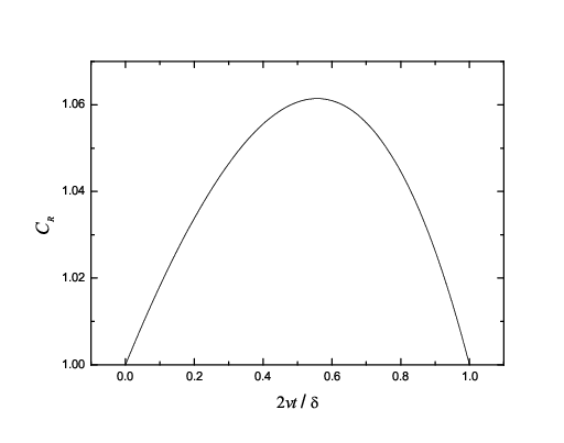
For this case, the complexity, $C_{R}$ , can be analytically obtained. Its expression is:

C_{R}(t)=\left\{\begin{array}[]{llc}2^{2vt/\delta}\left(1-{vt\over\delta}\right)&\mbox{if}&0\leq 2vt\leq\delta\,,\\ &\\ 1&\mbox{if}&2vt>\delta\,,\end{array}\right.

(9)

The behavior of $C_{R}$ as a function of the adimensional quantity $2vt/\delta$ is given in Fig. 5. Let us observe that $C_{R}$ presents a maximum. The shape of system (1) for this maximun complexity case is plotted in an adimensional scale in Fig. 6.

2.4 Triangular traveling densities

The two one-dimensional traveling densities that compose system (1) take the form in this case:

\rho_{\pm}(x,t)=\left\{\begin{array}[]{llc}{(x\mp vt)\over\epsilon^{2}}+{1\over\epsilon}&\mbox{if}&-\epsilon\leq x\mp vt\leq 0\,,\\ &&\\ {-(x\mp vt)\over\epsilon^{2}}+{1\over\epsilon}&\mbox{if}&0<x\mp vt\leq\epsilon\,,\\ &&\\ 0&\mbox{if}&|x\mp vt|>\epsilon\,,\end{array}\right.

(10)

where $\epsilon$ is the width of each distribution (isosceles triangle whose base length is $2\epsilon$ ).

The behavior of complexity, $C_{T}$ , as a function of the adimensional quantity $2vt/\epsilon$ is given in Fig. 7. Let us observe that $C_{T}$ presents a maximum and a minimum. The shape of system (1) for both cases, with maximum and minimum complexitiy, are plotted in an adimensional scale in Figs. 8 and 9, respectively.

2.5 Gamma traveling densities

We study a final case given by the crossing between two gamma distributions. Here the two one-dimensional traveling densities that compose system (1) take the form:

\rho_{\pm}(x,t)={1\over 2\theta^{k}\Gamma(k)}\,|x\mp vt|^{k-1}\exp\left\{{-{|x\mp vt|}/\theta}\right\},

(11)

where $k$ is a real parameter such that $k\geq 1$ and $\theta$ is a scale parameter related to the width of the distribution for a given $k$ . Observe that the exponential case is recovered for $k=1$ . Let us also remark that for a fixed $k$ the parameter $\theta$ modifies the shape of the distribution but the complexity $C$ is conserved.

The behavior of complexity, $C_{Gam}$ , as a function of the adimensional quantity $2vt/\theta$ is given in Fig. 10 for $k=3$ . The behavior for other values of $k$ seems to be similar. Let us observe that $C_{Gam}$ presents two local maxima and two local minima. The shape of system (1) for all these cases, with local extremal complexity, are plotted in an adimensional scale in Figs. 11 and 12, for the local maxima, and in Figs. 13 and 14, for the local minima.

3 Conclusion

In this work, we have studied the behavior of the statistical complexity as a function of time when two traveling identical densities are crossing each other. Five cases have been analyzed: Gaussian, exponential, rectangular, triangular and gamma densities. The Gaussian and exponential cases present a particular configuration with minimum complexity. The rectangular case displays a particular configuration with maximum complexity. The triangular case shows an intermediate behavior between the two former cases with two particular configurations, one of them with maximum complexity and the other one with minimum complexity. The gamma case displays two configurations with local minima complexity and other two configurations with local maxima complexity. In general, all these configurations with extremal complexity cannot be analytically obtained and a careful computational study is required in order to determine them.

Acknowledgment

This research was supported by the spanish Grant with Ref. FIS2009-13364-C02-C01. J.S. also thanks to the Consejería de Economía, Comercio e Innovación of the Junta de Extremadura (Spain) for financial support, Project Ref. GRU09011.

References

[1] \harvarditemCalbet \harvardand López-Ruiz2001calbet2001 Calbet, X. \harvardand López-Ruiz, R. \harvardyearleft2001\harvardyearright. Tendency toward maximum complexity in a non-equilibrium isolated system, Phys. Rev. E 63: 066116(9pp).
[2] \harvarditem[Catalán et al.]Catalán, Garay \harvardand López-Ruiz2002lopez2002 Catalán, R., Garay, J. \harvardand López-Ruiz, R. \harvardyearleft2002\harvardyearright. Features of the extension of a statistical measure of complexity to continuous systems, Phys. Rev. E 66: 011102(6pp).
[3] \harvarditem[Dembo et al.]Dembo, Cover \harvardand Thomas1991dembo1991 Dembo, A., Cover, T. \harvardand Thomas, J. \harvardyearleft1991\harvardyearright. Information theoretic inequalities, IEEE Trans. Inf. Theory 37: 1501–1518.
[4] \harvarditem[López-Ruiz et al.]López-Ruiz, Mancini \harvardand Calbet1995lopez1995 López-Ruiz, R., Mancini, H. \harvardand Calbet, X. \harvardyearleft1995\harvardyearright. A statistical measure of complexity, Phys. Lett. A 209: 321–326.
[5] \harvarditemLópez-Ruiz \harvardand Sañudo2010tunez2010 López-Ruiz, R. \harvardand Sañudo, J. \harvardyearleft2010\harvardyearright. Statistical complexity in traveling densities, Proceedings of the 9th WSEAS International NOLASC’10 Conference, Special Session ”Statistical Complexity in Classical and Quantum Systems”, Sousse, Tunisia -: 20–23.
[6] \harvarditemShannon1948shannon1948 Shannon, C. \harvardyearleft1948\harvardyearright. A mathematical theory of communication, Bell. Sys. Tech. J. 27: 379–423.

Shape of Traveling Densities with Extremum Statistical Complexity