Physics of extra dimensions is an interesting possibility of physics beyond the standard model [1]-[12]. As in a picture believed commonly, physical quantities are momentum-dependent so that quantum corrections should be considered. However, it is far from the full understanding when extra dimensions are included. There are problems of higher-dimensional theory. One arises from a property of non-renormalizability. This inevitably gives rise to innumerable higher-dimensional operators. Another is that loop integrals of virtual processes have higher degrees of divergence than the corresponding four-dimensional integrals. These problems are related to applicability of the theory to describe high-energy behavior. It may be prospective to claim that quantum effects in higher-dimensional theory are derived only in an ultraviolet completion. As such a circumstance, there are some calculations of extra-dimensional loop effects. In flat space, gauge couplings have linear divergence [13, 14]. In warped space, the divergence of gauge couplings is logarithmic [15, 16]. Taking into account the form of the background may give a clue to address the problem of high degrees of divergence for loop integrals.

Extra dimensions need to be hidden if they exist. At low energies spacetime is effectively in four dimensions and at high energies extra dimensions are visible or their signals are visible. It is possible to describe well this picture in a method of tracking the number of Kaluza-Klein (KK) modes [17, 18]. In this method, the coupling has linear dependence on the number of KK modes. At higher energies the number of KK modes is proportional to the cutoff so that dependence is linear to the cutoff. In a typical theory with flat extra dimensions, coupling constants quickly grow and become non-perturbative at about ${\cal O}(10)$ times larger than the KK scale. If the higher-dimensional theory is a perturbation theory only right above the KK scale, the region where it is regarded as a quantum field theory would be too small. Flat extra dimensions may not be suitable for perturbation theory of quantum fields in higher dimensions. In warped space, a position-dependent cutoff directly leads to extra-dimensional signals without tracking the number of KK modes. The pioneering idea with warped space was to generate the hierarchy by making the cutoff on the Planck brane be such a large scale as the Planck scale [10]. Here we stress it is nontrivial whether the idea of the hierarchy solution is compatible with the aspect that at the Planck scale gravity may be quantized. When the Planck scale is included in the context of a theory, the geometry does not appear to be fixed in a classical form. Therefore, if there is an extra-dimensional theory as a quantum theory without including quantization of gravity, the candidate might be a theory in warped space at an intermediate scale whose cutoff is much larger than the TeV scale and much less than the Planck scale.

In this paper, we study a quantum field theory in warped space at an intermediate scale between the TeV and the Planck scales. The intermediate scale is regarded as being much lower than the scale of the geometry stabilization or the Planck scale. In order to avoid the appearance of the Planck scale in the present framework, we place the intermediate and TeV branes at the ends of the bulk instead of the Planck and TeV branes. In dealing with the action integral of field theory, one of the important things is to have a guide of invariance of theory. On the one hand, Lorentz invariance in the bulk is explicitly broken. On the other hand, gauge invariance tends to be preserved at high energies [19]. In this light, we deal with gauge theory, although the estimation of the effect of the extra-dimensional Lorentz violation is beyond the scope of this paper. The vertices of our interest are interactions for low-mass states which are dynamical in effective theory. We examine vertex corrections to self-couplings where zero modes are in external lines. Introducing a position-dependent cutoff, we find that it is possible to perform diagrammatic calculations where the contributions include the effect of a virtual bulk propagation. The values of the corrections are not so different from the four-dimensional correspondent and this supports validity of perturbation at the intermediate scale. On the other hand, it is found that there is nontrivial dependence of the corrections on the curvature and the warp factor and that for a part of each diagram the coefficient for the logarithmic scaling has the value in the four-dimensional theory. In addition to the problem of validity of perturbation, we discuss the problem of higher-dimensional operators associated with non-renormalizability. Non-renormalizability is linked to infinite number of counterterms. We point out a direction to try to identify vertex corrections for low-mass states from higher-dimensional operators without knowing details about how higher-dimensional operators themselves are generated and receive corrections.

This paper is organized as follows. In Sec. 2, an outline of calculations of vertex corrections with a position-dependent cutoff is given. In Sec. 3, the model of non-Abelian theory in warped space is given. In Sec. 4, our result of loop corrections is shown. In Sec. 5, higher-dimensional operators are discussed. We conclude in Sec. 6. Details of Green functions and formula of Bessel functions are summarized in Appendices A and B, respectively.

Our interest in this paper is quantum aspects of vertices in five-dimensional spacetime. As two external lines correspond to propagators, the first vertex appears when the number of external lines is three. With taking into account a three-point vertex, we can imagine the further extension to multiple point diagrams and higher loop corrections. The treatment of two-point diagrams can be read from that of three-point diagrams so that the comparison of the two-point diagrams with the three-point diagrams is applied to the analysis of multiple point diagrams. In addition, in the four-dimensional theory the two-loop renormalization for two-point diagrams needs the one-loop counterterms for three-point diagrams.

For the external lines with fixed positions, their vertices are located at various positions in five-dimensional spacetime. In Figure 1, four-dimensional directions are denoted in vertical directions and the extra-dimensional direction is denoted in a horizontal direction.

Each vertex has corrections. As a practical way to deal with warped space, we adopt a position-dependent cutoff for four-momentum. This is important for keeping perturbative validity of coupling constants. Examples of one-loop diagrams are given in Figure 2. For the left and right figures for vertices in Figure 2, the momentum cutoffs of loop integral are taken differently from each other.

All of these position-dependent contributions must be summed up continuously, i.e., must be integrated.

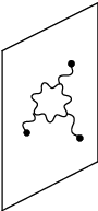
It is physically important to consider the situation that dynamical fields in effective theory below the TeV scale are external lines for three-point functions. For pure gauge theory without symmetry breaking, such dynamical fields are massless mode. The zero mode is a constant with respect to the position in the extra dimension. We will explicitly show in the next section that the Green function connecting a five-dimensional field to a four-dimensional zero mode is position-independent. Because of this position independence, loop corrections can be calculated for diagrams where external lines are amputated. For example, a one-loop diagram composed of three-point interactions is shown in Figure 3.

The cutoff for the four-momentum is determined by the largest interacting position $z$ shown as the vertical broken line in Figure 3. This diagram involves the loop- and $z$-integrals given by

$\displaystyle\int_{1}^{z_{L}}{dz\over kz}\int_{|\ell|\leq\Lambda_{z}}{d^{4}\ell\over(2\pi)^{4}}\int_{1}^{z}{dz_{1}\over kz_{1}}\int_{1}^{z}{dz_{2}\over kz_{2}}G_{\ell}(z,z_{1})G_{\ell}(z,z_{2})G_{\ell}(z_{1},z_{2})\times F,$

(2.1)

where a Green function is denoted as $G_{p}(z,z^{\prime})$ and it depends on four-momentum and the fifth-dimensional position. The factor $F$ is associated with momentum flow and it generally includes the loop momentum $\ell$. The position-dependent cutoff has been introduced as $\Lambda_{z}\equiv\Lambda z_{L}/z$. The momentum cutoff at $z=z_{L}$ is $\Lambda$ and is assumed as $\Lambda\simeq 10$TeV. For a small $z$, $\Lambda_{z}$ becomes large. The energy region of the theory depending on $z$ is schematically shown in Figure 4.

The loop four-momenta run up to the common energy scale, $\Lambda_{z}$ in Figure 4. The cutoff of the theory at a position and also the common energy scale do not need to reach the typical energy region of the theory at a different position, as seen for the theories at $z_{1}$ and $z$ in Figure 4. The other diagrams will be taken into account similarly.

In this section, we give the model and the resulting two-point functions and Green functions. The action integral for non-Abelian gauge theory is given by

$\displaystyle\int d^{4}x\int_{1}^{z_{L}}dz\sqrt{\textrm{det}(g_{KL})}\textrm{tr}\left(-{1\over 2}F_{MN}F_{PQ}g^{MP}g^{NQ}-{1\over\xi}\omega(A)^{2}\right)+S_{\textrm{\scriptsize ghost}},$

(3.1)

with the metric in the five-dimensional spacetime

$\displaystyle ds^{2}={1\over z^{2}}(\eta_{\mu\nu}dx^{\mu}dx^{\nu}-{1\over k^{2}}dz^{2}).$

(3.2)

The four-dimensional Minkowski metric is $(+1,-1,-1,-1)$. The extra-dimensional coordinate is denoted as $z$. The coordinate $z$ takes a value in $1\leq z\leq z_{L}\equiv e^{kL}$, where $k$ is the curvature and $L$ is the size of the extra dimension. The five-dimensional gauge field $A_{M}$ is parted into $A_{\mu}$ and $A_{z}$. The gauge fixing can be taken so as to remove kinetic mixing terms,

$\displaystyle\omega(A)=\partial_{\mu}A_{\nu}\cdot g^{\mu\nu}+\xi zg^{zz}\partial_{z}({1\over z}A_{z}).$

(3.3)

Correspondingly to this gauge fixing, the ghost action integral is given by

	$\displaystyle S_{\textrm{\scriptsize ghost}}$	$\displaystyle\!\!\!=\!\!\!$	$\displaystyle\int d^{4}x\int_{1}^{z_{L}}{dz\over kz}\left(\bar{c}^{a}(-\partial^{\mu}\partial_{\mu})c^{a}-gf^{abc}\bar{c}^{a}\partial^{\mu}(A_{\mu}^{b}c^{c})\right.$		(3.4)
			$\displaystyle\left.+\xi\bar{c}^{a}k^{2}z\partial_{z}({1\over z}\partial_{z})c^{a}+\xi gf^{abc}\bar{c}^{a}k^{2}z\partial_{z}({1\over z}A_{z}^{b}c^{c})\right).$

Here the contraction of a subscript with a superscript stands for a contraction with $\eta^{\mu\nu}$ such as $F_{\mu\nu}F^{\mu\nu}=F_{\mu\nu}F_{\rho\sigma}\eta^{\mu\rho}\eta^{\nu\sigma}$. A contraction with $g^{MN}$ is described explicitly with $g^{MN}$ such as $F_{\mu\nu}F_{\rho\sigma}g^{\mu\rho}g^{\nu\sigma}$. This rule will be used throughout this paper. From the action integral (3.1), interactions for $A_{\mu}$ and $A_{z}$ are given by

	$\displaystyle\int d^{4}x\int_{1}^{z_{L}}{dz\over kz}\left(-gf^{abc}\partial_{\mu}A_{\nu}^{a}\cdot A^{\mu b}A^{\nu c}-{1\over 4}g^{2}f^{abe}f^{cde}A_{\mu}^{a}A_{\nu}^{b}A^{\mu c}A^{\nu d}\right.$
	$\displaystyle\left.+k^{2}gf^{abc}(\partial_{\mu}A_{z}^{a}-\partial_{z}A_{\mu}^{a})\cdot A^{\mu b}A_{z}^{c}+{1\over 2}k^{2}g^{2}f^{abe}f^{cde}A_{\mu}^{a}A_{z}^{b}A^{\mu c}A_{z}^{d}\right).$		(3.5)

In the equation (3.5), the first term with three gauge fields being zero mode is the vertex of our interest. We will examine how the term receives corrections.

In order that symmetry group before the gauge fixing in four dimensions is identical with the original gauge group, $A_{\mu}$ and ghost fields obeys Neumann boundary condition and $A_{z}$ obeys Dirichlet boundary condition. From equations of motion and boundary conditions, the zero modes for $A_{\mu}$ and ghost are constants with respect to the extra-dimensional coordinate. The gauge field is expanded as

$\displaystyle A_{\mu}(x,z)={1\over\sqrt{L}}A_{\mu 0}(x)+\sum_{n=1}^{\infty}N_{n}A_{\mu n}(x)\chi_{n}(z),$

(3.6)

where $N_{n}$ is a normalization constant. For the $\xi=1$ gauge, massive-mode function $\chi_{n}$ for $A_{\mu}$ is given by

$\displaystyle\chi_{n}(z)=z(J_{1}({m_{n}z\over k})+\beta_{n}Y_{1}({m_{n}z\over k})),$

(3.7)

where $\beta_{n}=-J_{0}(m_{n}/k)/Y_{0}(m_{n}/k)=-J_{0}(m_{n}z_{L}/k)/Y_{0}(m_{n}z_{L}/k)$. The mode function $\phi_{n}$ for $A_{z}$ is given by $\phi_{n}(z)=(k/m_{n})\partial_{z}\chi_{n}(z)$.

The Green functions obeying the following equations can be introduced,

	$\displaystyle\left(\partial_{z}^{2}-{1\over z}\partial_{z}+{p^{2}\over k^{2}}\right)G_{p}(z,z^{\prime})={z\over k}\delta(z-z^{\prime}),$		(3.8)
	$\displaystyle\left(\partial_{z}^{2}-{1\over z}\partial_{z}+{p^{2}\over k^{2}\xi}\right)G_{p\over\sqrt{\xi}}(z,z^{\prime})={z\over k}\delta(z-z^{\prime}),$		(3.9)
	$\displaystyle\left(\partial_{z}^{2}-{1\over z}\partial_{z}+{1\over z^{2}}+{p^{2}\over k^{2}\xi}\right)S_{p\over\sqrt{\xi}}(z,z^{\prime})={z\over k}\delta(z-z^{\prime}).$		(3.10)

With these Green functions, two-point functions in the $\xi=1$ gauge for $A_{\mu}$, $A_{z}$ and ghost are given by

	$\displaystyle\langle\tilde{A}^{\mu a}(p,z^{\prime})\tilde{A}^{\nu b}(q,z)\rangle$	$\displaystyle\!\!\!=\!\!\!$	$\displaystyle\delta^{ab}(-iG_{p}(z,z^{\prime})\eta^{\mu\nu})(2\pi)^{4}\delta^{4}(p+q),$		(3.11)
	$\displaystyle\langle\tilde{A}_{z}^{a}(p,z^{\prime})\tilde{A}_{z}^{b}(q,z)\rangle$	$\displaystyle\!\!\!=\!\!\!$	$\displaystyle\delta^{ab}{1\over k^{2}}iS_{p}(z,z^{\prime})(2\pi)^{4}\delta^{4}(p+q),$		(3.12)
	$\displaystyle\langle\bar{\tilde{c}}^{a}(p,z^{\prime})\tilde{c}^{a}(q,z)\rangle$	$\displaystyle\!\!\!=\!\!\!$	$\displaystyle iG_{p}(z,z^{\prime})(2\pi)^{4}\delta^{4}(p+q),$		(3.13)

where the four-dimensional coordinates are written in a momentum picture via Fourier transformation. The explicit forms of Green functions are shown in Appendix A.

The two-point function for a five-dimensional gauge field and a four-dimensional zero-mode gauge field is found from the orthogonality of the mode function. The orthogonality of $\chi_{n}$ yields

$\displaystyle\int_{1}^{z_{L}}{dz\over kz}A_{\mu}(x,z){1\over\sqrt{L}}=A_{\mu 0}(x).$

(3.14)

With this property and the integral of the Green function

$\displaystyle\int_{1}^{z_{L}}{dz^{\prime}\over kz^{\prime}}G_{p}(z,z^{\prime})=\int_{1}^{z}{dz^{\prime}\over kz^{\prime}}G_{p}(z,z^{\prime})_{z^{\prime}\leq z}+\int_{z}^{z_{L}}{dz^{\prime}\over kz^{\prime}}G_{p}(z,z^{\prime})_{z^{\prime}\geq z}={1\over p^{2}},$

(3.15)

the two-point function for $A_{\mu}$ and $A_{\nu 0}$ is obtained as

$\displaystyle\langle\tilde{A}_{\mu}^{a}(p,z)\tilde{A}_{\nu 0}^{b}(q)\rangle={1\over\sqrt{L}}{1\over p^{2}}\delta^{ab}(2\pi)^{4}\delta^{4}(p+q)(-i\eta_{\mu\nu}).$

(3.16)

The two-point function (3.16) is independent of the position $z$.

For KK mode, the mode function has the $z$-dependence. In analogy with Eq. (3.15), the formula is given by

$\displaystyle\int_{1}^{z_{L}}{dz^{\prime}\over kz^{\prime}}G_{p}(z,z^{\prime})\chi_{n}(z^{\prime})={1\over p^{2}-m^{2}}\,\chi_{n}(z).$

(3.17)

From this equation, the two-point function for a five-dimensional gauge field and a four-dimensional KK-mode gauge field is obtained as

$\displaystyle\langle\tilde{A}_{\mu}^{a}(p,z)\tilde{A}_{\nu n}^{b}(q)\rangle=N_{n}\chi_{n}(z){1\over p^{2}-m^{2}}\delta^{ab}(2\pi)^{4}\delta^{4}(p+q)(-i\eta_{\mu\nu}).$

(3.18)

Diagrams with KK-mode external lines may be amputated with respect to the four-dimensional part, whereas the $z$-dependence such as $N_{n}\chi_{n}(z)$ in Eq. (3.18) needs to be taken into account in Eq. (2.1).

We calculate loop corrections of the three-point vertex in the model given in the previous section. For the one-loop diagrams, the tensor structure for momentum flow is analogous to the four-dimensional case. The Green function for gauge field is related to the four-dimensional gauge field propagator with the correspondence,

$\displaystyle-{i\eta_{\mu\nu}\over p^{2}}\leftrightarrow iG_{p}(z,z^{\prime})\eta_{\mu\nu},$

(4.1)

in the $\xi=1$ gauge. Using the same Feynman parameters as in four-dimensional case, we find the one-loop divergent part

$\displaystyle{\cal M}_{\textrm{\scriptsize 1-loop},\mu\nu\rho}^{abc}={1\over(4\pi)^{2}}{g^{3}\over L\sqrt{L}}C_{2}(G)f^{abc}V_{\mu\nu\rho}{\cal M}_{\textrm{\scriptsize 1-loop}},$

(4.2)

with

$\displaystyle{\cal M}_{\textrm{\scriptsize 1-loop}}=-2\left[\left({13\over 8}-{1\over 24}\right){U_{1}\over 2}-{9\over 4}U_{2}\right],$

(4.3)

where the factors $13/8$, $-1/24$ and $-9/4$ arise from three-point interactions, a ghost loop and the contribution with a four-point interaction, respectively. The tensor structure for the momentum flow of the external lines is given by

$\displaystyle V_{\mu\nu\rho}=(q+2p)_{\nu}\eta_{\mu\rho}-(p+2q)_{\mu}\eta_{\nu\rho}+(q-p)_{\rho}\eta_{\mu\nu}.$

(4.4)

The loop- and $z$-integrals are included in

	$\displaystyle i{2\over(4\pi)^{2}}U_{1}$	$\displaystyle\!\!\!=\!\!\!$	$\displaystyle\int_{1}^{z_{L}}{dz\over kz}\int_{|\ell|\leq\Lambda_{z}}{d^{4}\ell\over(2\pi)^{4}}\int_{1}^{z}{dz_{1}\over kz_{1}}\int_{1}^{z}{dz_{2}\over kz_{2}}G_{\ell}(z,z_{1})G_{\ell}(z,z_{2})G_{\ell}(z_{1},z_{2})\ell^{2},$		(4.5)
	$\displaystyle i{2\over(4\pi)^{2}}U_{2}$	$\displaystyle\!\!\!=\!\!\!$	$\displaystyle\int_{1}^{z_{L}}{dz\over kz}\int_{|\ell|\leq\Lambda_{z}}{d^{4}\ell\over(2\pi)^{4}}\int_{1}^{z}{dz_{1}\over kz_{1}}(G_{\ell}(z,z_{1}))^{2}.$		(4.6)

These needs to be examined with a numerical analysis. Then ${\cal M}_{\textrm{\scriptsize 1-loop}}$ is obtained. The correspondence of $U_{1}$ and $U_{2}$ with the four-dimensional case is

	$\displaystyle U_{1}$	$\displaystyle\!\!\!\leftrightarrow\!\!\!$	$\displaystyle\left[i{2\over(4\pi)^{2}}\right]^{-1}\int{d^{4}\ell\over(2\pi)^{4}}{2\ell^{2}\over\left[\ell^{2}-\Delta\right]^{3}}=\log\left(\Lambda^{2}\over\Delta\right),$		(4.7)
	$\displaystyle U_{2}$	$\displaystyle\!\!\!\leftrightarrow\!\!\!$	$\displaystyle\left[i{2\over(4\pi)^{2}}\right]^{-1}\int{d^{4}\ell\over(2\pi)^{4}}{1\over\left[\ell^{2}-\Delta\right]^{2}}={1\over 2}\log\left(\Lambda^{2}\over\Delta\right),$		(4.8)

where $\sqrt{|\Delta|}$ has the scale of external momenta. The four-dimensional correspondent for Eq. (4.3) is given by

$\displaystyle{\cal M}_{\textrm{\scriptsize 1-loop}}\leftrightarrow{2\over 3}\log\left({\Lambda^{2}\over\Delta}\right)\simeq{4\over 3}\log\left({10\textrm{TeV}\over 100\textrm{GeV}}\right)={8\over 3}\log 10.$

(4.9)

Since the momentum-dependence of Eq. (4.9) is logarithmic, the order of the value is not sensitive to a choice of the value of $\Delta$.

Now we analyze $U_{1}$ given in Eq. (4.7). After the $z_{1}$ and $z_{2}$ integrals and the Wick rotation, $U_{1}$ is written as

$\displaystyle U_{1}$

$\displaystyle\!\!\!=\!\!\!$

$\displaystyle-\int_{1}^{z_{L}}{dz\over kz}\int_{0}^{\Lambda_{z}}d\ell_{E}I_{G3}(z)\ell_{E}^{5},$

(4.10)

where the integral of the product of the Green functions is given by

	$\displaystyle I_{G3}(z)$	$\displaystyle\!\!\!=\!\!\!$	$\displaystyle{1\over k^{5}}\bigg\{-{\bar{N}^{2}\over 8}(\bar{d}_{1}(z))^{2}{1\over P_{E}^{2}}\left[{4\bar{N}\over\pi^{2}}T(1)+2a_{0}(z)a_{2}(z)\right.$		(4.11)
			$\displaystyle\left.-\bar{N}P_{E}^{2}T(z)\left[(\bar{a}_{1}(z))^{2}+a_{0}(z)a_{1}(z)\right]\right]\bigg\}.$

The functions appearing in Eq. (4.11) are written in terms of the modified Bessel functions as

	$\displaystyle\bar{N}$	$\displaystyle\!\!\!=\!\!\!$	$\displaystyle{\pi^{2}\over 4}{1\over K_{0}(P_{E})I_{0}(P_{E}z_{L})-I_{0}(P_{E})K_{0}(P_{E}z_{L})},$		(4.12)
	$\displaystyle\bar{d}_{1}(z)$	$\displaystyle\!\!\!=\!\!\!$	$\displaystyle{2\over\pi}z\left[K_{0}(P_{E}z_{L})I_{1}(P_{E}z)+I_{0}(P_{E}z_{L})K_{1}(P_{E}z)\right],$		(4.13)
	$\displaystyle T(z)$	$\displaystyle\!\!\!=\!\!\!$	$\displaystyle-2\bar{a}_{1}(z)\bar{d}_{1}(z)-a_{0}(z)d_{2}(z)-a_{2}(z)d_{0}(z),$		(4.14)
	$\displaystyle d_{0}(z)$	$\displaystyle\!\!\!=\!\!\!$	$\displaystyle{2\over\pi}z\left[K_{0}(P_{E}z_{L})I_{0}(P_{E}z)-I_{0}(P_{E}z_{L})K_{0}(P_{E}z)\right],$		(4.15)
	$\displaystyle d_{2}(z)$	$\displaystyle\!\!\!=\!\!\!$	$\displaystyle{2\over P_{E}z}\bar{d}_{1}(z)-d_{0}(z),$		(4.16)

where $\ell_{E}$ denotes the length in the polar coordinate and $P_{E}=\ell_{E}/k$. The functions $a_{i}(z)$ are given by $d_{i}(z)$ with the replacement $z_{L}\to 1$. The detail of the derivation of Eq. (4.11) is shown in Appendix A. Similarly $U_{2}$ is obtained as

$\displaystyle U_{2}=\int_{1}^{z_{L}}{dz\over kz}\int_{0}^{\Lambda_{z}}d\ell_{E}I_{G2}(z,z)\ell_{E}^{3},$

(4.17)

where

$\displaystyle I_{G2}(z,z)={1\over k^{3}}\left\{{1\over 2}\bar{N}^{2}(\bar{d}_{1}(z))^{2}\left[(\bar{a}_{1}(z))^{2}+a_{0}(z)a_{2}(z)-{4\over\pi^{2}P_{E}^{2}}\right]\right\}.$

(4.18)

We evaluate $\bar{U}_{1}=U_{1}/\log z_{L}$ and $\bar{U}_{2}=U_{2}/\log z_{L}$ changing the values of $k$ and $z_{L}$. These values are order ${\cal O}(1)$ at scales much larger than the TeV scale such as $\Lambda_{z}|_{z=1}=10^{11}\textrm{GeV}$ for $z_{L}=10^{7}$. The numerical values of $\bar{U}_{j}$, $j=1,2$ are tabulated in Table 1.

From Eqs. (4.7) and (4.8), the four-dimensional correspondents satisfy $U_{1}=2U_{2}$. The contributions in the warped space tend to have

$\displaystyle U_{1}={1\over 2}\bar{U}_{1}\log z_{L}^{2}<2U_{2}=\bar{U}_{2}\log z_{L}^{2},$

(4.19)

The correspondence between the values in the four-dimensional case and the warped case occurs depending on $k$ and $z_{L}$. The value $\bar{U}_{1}\approx 1$ is generated for a relatively small $k/z_{L}$. The value $\bar{U}_{2}\approx 0.5$ is generated for a large $z_{L}$ and a relatively large $k/z_{L}$. Once the factor $U_{1}$ and $U_{2}$ are obtained, the contribution ${\cal M}_{\textrm{\scriptsize 1-loop}}$ is derived from Eq. (4.3). The behavior of $\overline{\cal M}_{\textrm{\scriptsize 1-loop}}={\cal M}_{\textrm{\scriptsize 1-loop}}/\log z_{L}^{2}$ as a function of $\bar{U_{j}}$ is shown in Figure 5.

It is seen that the value $\overline{\cal M}_{\textrm{\scriptsize 1-loop}}$ can be positive or negative in a region of $\bar{U}_{j}\sim{\cal O}(1)$. The numerical values of $\overline{\cal M}_{\textrm{\scriptsize 1-loop}}$ for the parameters $z_{L}$ and $k$ given in Table 1 are tabulated in Table 2.

The value of $\overline{\cal M}_{\textrm{ \scriptsize 1-loop}}$ is order ${\cal O}(1)$ and the explicit dependence of the correction ${\cal M}_{\textrm{ \scriptsize 1-loop}}$ on the warp factor is logarithmic, $\log z_{L}^{2}$. In this sense, the perturbation including bulk contributions is valid even at scales which are the warp factor times larger than the TeV scale. The value $\overline{\cal M}_{\textrm{\scriptsize 1-loop}}\approx 2/3$ is obtained for a large $z_{L}$ and a relatively large $k/z_{L}$ where $U_{2}$ in Eq. (4.3) is close to the four-dimensional value and $U_{1}$ is relatively small. The feature of the result is summarized as follows. On the one hand, it is found that the value of the factor $\overline{\cal M}_{\textrm{ \scriptsize 1-loop}}$ in Table 2 is not so different from $2/3$ in the four-dimensional case irrespective of the relation (4.19). On the other hand, each diagrams to compose the total contribution can give the same value as in the four-dimensional case.

Since the gauge coupling is negative mass dimension $[g]=[\textrm{mass}]^{-1/2}$, gauge-invariant higher-dimensional operators can be infinitely written down. This effect would need to be taken into account and the action integral is generally written as

$\displaystyle\int d^{4}x\int dz\sum_{d=0}^{\infty}\sum_{i}c_{d,i}g^{2d}{\cal O}_{d+5,i},$

(5.1)

where ${\cal O}_{D,i}$ denote a operator with dimension $[\textrm{mass}]^{D}$ for species $i$ and $c_{d,i}$ is the corresponding coefficient. However, it is unclear whether all $c_{d,i}$ can be fixed in the present framework. We would like to achieve any approach to identify corrections to low-energy interactions with leaving part of $c_{d,i}$ unknown. We have examined corrections for the zero-mode interaction in the mode expansion of the three-point interaction in Eq. (3.5),

$\displaystyle\int d^{4}x\left(-{g\over\sqrt{L}}f^{abc}\partial_{\mu}A_{\nu 0}^{a}\cdot A_{0}^{\mu b}A_{0}^{\nu c}\right).$

(5.2)

If higher-dimensional operators exist, they contribute to this vertex. For example, there would be dimension-seven operators

$\displaystyle c_{2,1}D^{P}D_{P}F_{MN}\cdot F^{MN}+c_{2,2}D^{M}D_{P}F_{MN}\cdot F^{PN}+\cdots.$

(5.3)

For simplicity, we assume that $c_{2,1}$ is dominant over the other coefficients. Then propagator has an extra factor $1/(c_{2,1}p^{2})$ for a large momentum. In addition, three-point and four-point vertices have an extra factor $c_{2,1}p^{2}$ for a large momentum. Because the propagator is suppressed by an extra factor, the divergent correction to Eq. (5.2) arises not from the original dimension-five operators but from the dimension-seven operators. One-loop diagrams are the same form as drawn by the original dimension-five operators. The diagram composed of only three-point vertex has three internal propagators and three vertices. The ghost loop is similar. The diagram including four-point vertex has two internal propagators and two vertices. Therefore, the extra factors in the propagator and the vertices are canceled each other in the diagrams.

This is depicted in Figure 6. Then we do not need to know what the value of the coefficient $c_{2,1}$ is. Although the idea here is not a solution of the problem of higher-dimensional operators, further development might lead to a method to bypath the problem of higher-dimensional operators.

We have studied a quantum field theory in warped space at an intermediate scale between the TeV and the Planck scales. Our point has been to avoid the appearance of the Planck scale in the present framework by placing the intermediate and TeV branes at the ends of the bulk instead of the Planck and TeV branes. For this setup, we have examined vertex corrections to self-coupling where zero modes are in external lines. In the present case, zero mode is dynamical below the TeV scale. The effect of a position-dependent cutoff has been included via the extra-dimensional integral. The cutoff for the four-momentum $\Lambda_{z}=\Lambda z_{L}/z$ is determined by the smallest interacting point $z$. It has been shown that there is also a technical advantage with zero mode in external lines. The Green function connecting a five-dimensional field to a four-dimensional zero mode is position-independent so that calculations are performed for amputated diagrams. After integrals of products of the five-dimensional Green functions, we have found the vertex correction ${\cal M}_{\textrm{ \scriptsize 1-loop}}$ which depends on the curvature and the warp factor. The values of the corrections are not so different from the four-dimensional correspondent. Its explicit dependence on the warp factor is logarithmic, $\log z_{L}^{2}$. This supports validity of perturbation at the intermediate scale. As for the correspondence with the four-dimensional theory, the value $\bar{U}_{1}\approx 1$ is generated for a relatively small $k/z_{L}$. The values $\bar{U}_{2}\approx 0.5$ and $\overline{M}_{\textrm{\scriptsize 1-loop}}\approx 2/3$ are generated for a large $z_{L}$ and a relatively large $k/z_{L}$. In addition to the issue of perturbation, we have discussed the problem of higher-dimensional operators associated with non-renormalizability. We have pointed out the possibility that the extra factor originated from a higher-dimensional operator is canceled in the loop diagrams for the zero-mode self-coupling vertex. It still remains to examine higher-dimensional aspects from various viewpoints. It needs to be investigated further how a higher-dimensional theory can be a quantum field theory.

References

- [1] N. S. Manton, Nucl. Phys. B 158, 141 (1979).
- [2] D. B. Fairlie, Phys. Lett. B 82, 97 (1979).
- [3] D. B. Fairlie, J. Phys. G 5, L55 (1979).
- [4] Y. Hosotani, Phys. Lett. B 126, 309 (1983).
- [5] Y. Hosotani, Phys. Lett. B 129, 193 (1983).
- [6] I. Antoniadis, Phys. Lett. B 246, 377 (1990).
- [7] N. Arkani-Hamed, S. Dimopoulos and G. R. Dvali, Phys. Lett. B 429, 263 (1998) [arXiv:hep-ph/9803315].
- [8] I. Antoniadis, N. Arkani-Hamed, S. Dimopoulos and G. R. Dvali, Phys. Lett. B 436, 257 (1998) [arXiv:hep-ph/9804398].
- [9] H. Hatanaka, T. Inami and C. S. Lim, Mod. Phys. Lett. A 13, 2601 (1998) [arXiv:hep-th/9805067].
- [10] L. Randall and R. Sundrum, Phys. Rev. Lett. 83, 3370 (1999) [arXiv:hep-ph/9905221].
- [11] L. Randall and R. Sundrum, Phys. Rev. Lett. 83, 4690 (1999) [arXiv:hep-th/9906064].
- [12] T. Appelquist, H. C. Cheng and B. A. Dobrescu, Phys. Rev. D 64, 035002 (2001) [arXiv:hep-ph/0012100].
- [13] K. R. Dienes, E. Dudas and T. Gherghetta, Phys. Lett. B 436, 55 (1998) [arXiv:hep-ph/9803466].
- [14] K. R. Dienes, E. Dudas and T. Gherghetta, Nucl. Phys. B 537, 47 (1999) [arXiv:hep-ph/9806292].
- [15] A. Pomarol, Phys. Rev. Lett. 85, 4004 (2000) [arXiv:hep-ph/0005293].
- [16] L. Randall and M. D. Schwartz, JHEP 0111, 003 (2001) [arXiv:hep-th/0108114].
- [17] G. Bhattacharyya, A. Datta, S. K. Majee and A. Raychaudhuri, Nucl. Phys. B 760, 117 (2007) [arXiv:hep-ph/0608208].
- [18] N. Uekusa, Phys. Rev. D 75, 064014 (2007) [arXiv:hep-th/0701159].
- [19] N. Uekusa, arXiv:1004.4410 [hep-ph].