跳到论文正文
W Papers独立论文阅读器 arXiv:1006.5478 论文正文 计算阅读时间 · 0%
引用这篇论文根据当前论文元数据生成,正式投稿前建议核对。


License: arXiv.org perpetual non-exclusive license
arXiv:1006.5478v1 [math.SP] 28 Jun 2010

Sharp geometric upper bounds on resonances for surfaces with hyperbolic endsThanks: Supported in part by NSF grant DMS-0901937.

David Borthwick Address: Department of Mathematics and Computer Science, Emory University, Atlanta, Georgia, 30322, USA Email address: davidb@mathcs.emory.edu
Date: August 24, 2026
Abstract.

We establish a sharp geometric constant for the upper bound on the resonance counting function for surfaces with hyperbolic ends. An arbitrary metric is allowed within some compact core, and the ends may be of hyperbolic planar, funnel, or cusp type. The constant in the upper bound depends only on the volume of the core and the length parameters associated to the funnel or hyperbolic planar ends. Our estimate is sharp in that it reproduces the exact asymptotic constant in the case of finite-area surfaces with hyperbolic cusp ends, and also in the case of funnel ends with Dirichlet boundary condtiions.

2000 Mathematics Subject Classification
Primary 58J50, 35P25; Secondary 47A40

1. Introduction

For a compact Riemannian surface, the Weyl law shows that the asymptotic distribution of eigenvalues is determined by global geometric quantities. In the compact hyperbolic case, Weyl asymptotics follow easily from the Selberg trace formula, see e.g. [10], and this approach extends also to non-compact hyperbolic surfaces of finite area [15]. Some reinterpretation of the spectral counting is needed for the non-compact case; one can either supplement the counting function for the discrete spectrum by a term related to the scattering phase, or else use the counting function for resonances instead of eigenvalues. Weyl asymptotics, in this extended sense, were established for general finite-area surfaces with hyperbolic cusp ends by Müller [11] and Parnovski [13].

For infinite-area surfaces with hyperbolic ends, the discrete spectrum is finite and possibly empty, and therefore plays no role in the spectral asymptotics. One could look for analogies to the finite-area results in the asymptotics of either the scattering phase or the resonance counting function. For the scattering phase of a surface with hyperbolic ends, Weyl asymptotics were proven by Guillopé-Zworski [9]. One does not necessarily expect a corresponding result to hold for the resonance counting function—see e.g. [9, Remark 1.6], but neither can we rule out the possibility at this point. The issue of how global geometric properties influence the distribution of resonances a remains a compelling problem.

At present, only the order of growth of the resonance counting function is well understood. Guillopé-Zworski [8, 9] showed the the resonance counting function for infinite-area surfaces with hyperbolic ends satisfies Ng​(t)≍t2N_{g}(t)\asymp t^{2} (with the caveat that the lower bound is proportional to the 00-volume which might be zero in exceptional cases). These results have been extended to higher dimensional manifolds with hyperbolic ends in Borthwick [3]. Unfortunately, the methods used in these proofs yield only an ineffective constant for the upper bound, with no clear geometric content. Moreover, the derivation of the lower bound depends explicitly on the upper bound, so the geometric dependence of the lower bound was likewise unknown.

In this paper we present a geometric constant for the upper bound on the resonance counting function for infinite-area surfaces with hyperbolic ends. This constant is sharp in the sense that it agrees with the exact asymptotics in the cases of finite area surfaces or truncated funnnels. Our approach is inspired by Stefanov’s recent paper [14] on compactly supported perturbations of the Laplacian on ℝn\mathbb{R}^{n} for nn odd, and similar techniques were applied to compactly supported perturbations of ℍn+1\mathbb{H}^{n+1} in Borthwick [4].

We can state the cleanest result for a hyperbolic surface (X,g)≅ℍ2/Γ(X,g)\cong\mathbb{H}^{2}/\Gamma. Let ℛg\mathcal{R}_{g} denote the associated resonance set (poles of the meromorphic continuation of (Δg−s⁡(1−s))−1(\Delta_{g}-s(1-s))^{-1}), with counting function

Ng​(t):=#⁡{ζ∈ℛg:|ζ−12|≤t}.N_{g}(t):=\#\bigl\{\zeta\in\mathcal{R}_{g}:\>|\zeta-\tfrac{1}{2}|\leq t\bigr\}.

The sharp version of our bound involves a regularization of the counting function,

(1.1) N~g​(a):=∫0a2​Ng​(t)t2​𝑑t.\widetilde{N}_{g}(a):=\int_{0}^{a}\frac{2N_{g}(t)}{t^{2}}\>dt.

This type of regularization is standard in the theory of zeros of entire functions, and there is a natural connection to the asymptotics of Ng​(t)N_{g}(t),

N~g(a)∼Ba2⟺Ng(t)∼Bt2.\widetilde{N}_{g}(a)\sim Ba^{2}\quad\Longleftrightarrow\quad N_{g}(t)\sim Bt^{2}.

(see [14, Lemma 1]). If we work only with upper bounds, then we lose some sharpness in the estimate,

N~g​(a)≤B​a2⟹Ng​(t)≤e​B​t2.\widetilde{N}_{g}(a)\leq Ba^{2}\quad\Longrightarrow\quad N_{g}(t)\leq eBt^{2}.
Theorem 1.1.

Suppose (X,g)(X,g) is a geometrically finite hyperbolic surface with χ⁡(X)<0\chi(X)<0. Let ℓ1,…,ℓnf\ell_{1},\dots,\ell_{n_{\rm f}} denote the diameters of the geodesic boundaries of the funnels of XX. The regularized counting function for the resonances of Δg\Delta_{g} satisfies

(1.2) N~g​(a)a2≤|χ⁡(X)|+∑j=1nfℓj4+o⁡(1).\frac{\widetilde{N}_{g}(a)}{a^{2}}\leq|\chi(X)|+\sum_{j=1}^{n_{\rm f}}\frac{\ell_{j}}{4}+o(1).

We can see that this result is sharp in two extreme cases. For a finite-area hyperbolic surface (i.e. nf=0{n_{\rm f}}=0), our upper bound agrees with the known asymptotic Ng​(t)/t2∼|χ⁡(X)|N_{g}(t)/t^{2}\sim|\chi(X)|. Moreover, for an isolated hyperbolic funnel FℓF_{\ell} of boundary length ℓ\ell, under Dirichlet boundary conditions, the resonances form a half-lattice. It’s then easy to see that NFℓ​(t)/t2∼ℓ/4N_{F_{\ell}}(t)/t^{2}\sim\ell/4, so the funnel portion of (1.2) is also sharp.

The restriction to χ⁡(X)<0\chi(X)<0 in Theorem 1.1 leaves out just a few cases. The complete (smooth) hyperbolic surfaces for which χ⁡(X)≥0\chi(X)\geq 0 are the hyperbolic plane ℍ2\mathbb{H}^{2}, the hyperbolic cylinder Cℓ:=ℍ2/⟨z↦eℓ​z⟩C_{\ell}:=\mathbb{H}^{2}/\langle z\mapsto e^{\ell}z\rangle, and the parabolic cylinder C∞:=ℍ2/⟨z↦z+1⟩C_{\infty}:=\mathbb{H}^{2}/\langle z\mapsto z+1\rangle. Resonance sets can be computed explicitly in these cases, and exact asymptotics for the counting function are easily obtained:

Nℍ2​(t)∼t2,NCℓ​(t)∼ℓ2​t2,NC∞​(t)=1.N_{\mathbb{H}^{2}}(t)\sim t^{2},\qquad N_{C_{\ell}}(t)\sim\frac{\ell}{2}t^{2},\qquad N_{C_{\infty}}(t)=1.

If we interpret CℓC_{\ell} as the union of 2 funnel ends, then (1.2) would also give a sharp estimate for this case.

Using Theorem 1.1 in conjunction with the Guillopé-Zworski argument [9] for the lower bound, we can deduce the following:

Corollary 1.2.

For k∈ℕk\in\mathbb{N} there exists a constant ckc_{k} such that for any geometrically finite hyperbolic surface (X,g)(X,g) with χ⁡(X)<0\chi(X)<0,

Ng​(t)t2≥ck​|χ⁡(X)|​(1+1|χ⁡(X)|​∑j=1nfℓj4)−2k,\frac{N_{g}(t)}{t^{2}}\geq c_{k}\>|\chi(X)|\>\Biggl(1+\frac{1}{|\chi(X)|}\sum_{j=1}^{n_{\rm f}}\frac{\ell_{j}}{4}\Biggr)^{-\frac{2}{k}},

for t≥1t\geq 1.

The constant ckc_{k} obtained in this way (see §4 for the derivation) is rather ineffective; the point here is just that we can find a lower bound that depends only on χ⁡(X)\chi(X) and {ℓj}\{\ell_{j}\}.

We will obtain Theorem 1.1 as a consequence of a somewhat more general estimate. Consider a smooth Riemannian surface (X,g)(X,g), possibly with boundary, which has finitely many ends that are assumed to be of hyperbolic planar, funnel, or cusp type. That is, XX admits the following decomposition, as illustrated in Figure 1,

(1.3) X=K⊔Y1⊔⋯⊔Ynf⊔Cnf+1⊔⋯⊔Cnf+nc,X=K\sqcup Y_{1}\sqcup\dots\sqcup Y_{{n_{\rm f}}}\sqcup C_{{n_{\rm f}}+1}\sqcup\dots\sqcup C_{{n_{\rm f}}+{n_{\rm c}}},

where the core KK is a compact manifold with boundary. The metric in KK is arbitrary. The YjY_{j}’s are infinite-area ends: either hyperbolic planar,

(1.4) Yj≅[bj,∞)×S1,g|Yj=d​r2+sinh2⁡r​d​θ2,bj≥0,Y_{j}\cong[b_{j},\infty)\times S^{1},\quad g|_{Y_{j}}=dr^{2}+\sinh^{2}r\>d\theta^{2},\quad b_{j}\geq 0,

or hyperbolic funnels,

(1.5) Yj≅[bj,∞)×S1,g|Yj=dr2+ℓj2cosh2rd​θ2(2​π)2,bj,ℓj≥0.Y_{j}\cong[b_{j},\infty)\times S^{1},\quad g|_{Y_{j}}=dr^{2}+\ell_{j}^{2}\cosh^{2}r\frac{d\theta^{2}}{(2\pi)^{2}},\quad b_{j},\ell_{j}\geq 0.

The CjC_{j}’s are hyperbolic cusps,

(1.6) Cj≅[bj,∞)×S1,g|Cj=d​r2+e−2​r​d​θ2(2​π)2,bj≥0.C_{j}\cong[b_{j},\infty)\times S^{1},\quad g|_{C_{j}}=dr^{2}+e^{-2r}\frac{d\theta^{2}}{(2\pi)^{2}},\quad b_{j}\geq 0.

The finite-area portion of XX consisting of the core plus the cusps is denoted by

(1.7) Xc:=K⊔Cnf+1⊔⋯⊔Cnf+nc.X_{\rm c}:=K\sqcup C_{{n_{\rm f}}+1}\sqcup\dots\sqcup C_{{n_{\rm f}}+{n_{\rm c}}}.
Refer to caption
Figure 1. Surface XX with boundary and hyperbolic ends.

Note that any geometrically finite hyperbolic surface, with the exception of the parabolic cylinder C∞C_{\infty}, admits a decomposition of the form (1.3). And in such surfaces, aside from ℍ2\mathbb{H}^{2} itself, only funnel or cusp ends can occur.

We let Δg\Delta_{g} denote the positive Laplacian on (X,g)(X,g). In general we may consider the operator

P:=Δg+V,P:=\Delta_{g}+V,

where V∈C0∞​(X)V\in C^{\infty}_{0}(X) with supp⁡(V)⊂K\operatorname{supp}(V)\subset K. We denote by ℛP\mathcal{R}_{P} the resonance set associated to PP. These resonances are the poles of the analytically continued resolvent

RP​(s):=(P−s⁡(1−s))−1,R_{P}(s):=(P-s(1-s))^{-1},

counted according to multiplicity. The associated resonance counting function is

NP​(t):=#⁡{ζ∈ℛP:|ζ−12|≤t}.N_{P}(t):=\#\bigl\{\zeta\in\mathcal{R}_{P}:\>|\zeta-\tfrac{1}{2}|\leq t\bigr\}.

Our context is essentially that of Guillopé-Zworski [8, 9], and so we already know that NP​(t)≍t2N_{P}(t)\asymp t^{2} (see §2 for details). It is thus natural to define the regularized counting function N~P​(a)\widetilde{N}_{P}(a) just as in (1.1).

Before stating the upper bound, we introduce the asymptotic constants associated to the resonance count for isolated hyperbolic planar or funnel ends.

Theorem 1.3.

For a hyperbolic planar or funnel end Y≅[b,∞)×S1Y\cong[b,\infty)\times S^{1}, with metric as in (1.4) or (1.5), the resonance counting function for the Laplacian with Dirichlet boundary conditions at r=br=b satisfies an asymptotic as t→∞t\to\infty,

NY​(t)∼A⁡(Y)​t2.N_{Y}(t)\sim A(Y)t^{2}.

We will write these constants A⁡(Y)A(Y) explicitly in a moment. But first let us state the main result of this paper.

Theorem 1.4.

For (X,g)(X,g) a surface with hyperbolic ends as in (1.3), and V∈C0∞​(X)V\in C^{\infty}_{0}(X), the regularized counting function for P=Δg+VP=\Delta_{g}+V satisfies

(1.8) N~P​(a)a2≤12​π​vol⁡(Xc,g)+∑j=1nfA⁡(Yj)+o⁡(1),\frac{\widetilde{N}_{P}(a)}{a^{2}}\leq\frac{1}{2\pi}\operatorname{vol}\bigl(X_{\rm c},g\bigr)+\sum_{j=1}^{n_{\rm f}}A(Y_{j})+o(1),

where XcX_{\rm c} is the subset (1.7).

If (X,g)(X,g) is a finite-area surface with hyperbolic cusp ends (and arbitrary metric in the interior) Parnovski [13] proved that

Ng​(t)∼12​π​vol⁡(X,g)​t2.N_{g}(t)\sim\frac{1}{2\pi}\operatorname{vol}(X,g)t^{2}.

This shows that Theorem 1.4 is sharp in the case nf=0{n_{\rm f}}=0. It also suggests an intriguing interpretation of the constants appearing in (1.8). Suppose we split XX into a disjoint union Xc∪Y1∪⋯∪YnfX_{\rm c}\cup Y_{1}\cup\dots\cup Y_{n_{\rm f}} at the boundary of XcX_{\rm c} and impose Dirichlet boundary conditions at the newly created boundaries. The constant on the right-hand side of (1.8) is the sum of the asymptotic constants for the resonance counting function of the resulting components.

To obtain Theorem 1.1 from Theorem 1.4, we take the YjY_{j}’s to be standard funnels with boundaries at bj=0b_{j}=0. As mentioned above, A⁡(Yj)=ℓj/4A(Y_{j})=\ell_{j}/4 in that case. And since XcX_{\rm c} has geodesic boundary and hyperbolic interior, Gauss-Bonnet gives vol⁡(Xc,g)=−2​π​χ​(X)\operatorname{vol}(X_{\rm c},g)=-2\pi\chi(X).

As in Corollary 1.2, combining Theorem 1.4 with the Guillopé-Zworski argument gives a lower bound on NP​(t)N_{P}(t) with a constant that depends only on 0−vol⁡(X,g)\operatorname{0-vol}(X,g) and the end parameters ℓj\ell_{j} and bjb_{j} for j=1,…,nfj=1,\dots,{n_{\rm f}}, assuming that 0−vol⁡(X,g)≠0\operatorname{0-vol}(X,g)\neq 0.

The asymptotic constants A⁡(Y)A(Y) appearing in Theorem 1.3 have a somewhat complicated form. Consider first a model funnel end Fℓ,r0F_{\ell,r_{0}} defined by

(1.9) Fℓ,r0≅[r0,∞)×S1,d​s2=d​r2+ℓ2​cosh2⁡r​d​θ2(2​π)2.F_{\ell,r_{0}}\cong[r_{0},\infty)\times S^{1},\quad ds^{2}=dr^{2}+\ell^{2}\cosh^{2}r\frac{d\theta^{2}}{(2\pi)^{2}}.

The case r0=0r_{0}=0, a standard funnel with geodesic boundary, is simply denoted by FℓF_{\ell}. The resonance set for the Laplacian on Fℓ,r0F_{\ell,r_{0}} with Dirichlet boundary conditions at r=r0r=r_{0} is denoted ℛFℓ,r0\mathcal{R}_{F_{\ell,r_{0}}}.

In §7 we will show that for r0≥0r_{0}\geq 0,

(1.10) A(Fℓ,r0)=−ℓ2​πsinhr0+4π∫0π2∫0∞[I⁡(x​ei​θ,ℓ,r0)]+x3dxdθ,A(F_{\ell,r_{0}})=-\frac{\ell}{2\pi}\sinh r_{0}+\frac{4}{\pi}\int_{0}^{\frac{\pi}{2}}\int_{0}^{\infty}\frac{[I(xe^{i\theta},\ell,r_{0})]_{+}}{x^{3}}\>dx\>d\theta,

where [⋅]+[\cdot]_{+} denotes the positive part and, with ω:=2​π/ℓ\omega:=2\pi/\ell,

(1.11) I⁡(α,ℓ,r):=Re⁡[2​α​log⁡(α​sinh⁡r+ω2+α2​cosh2⁡rω2+α2)]+ω​arg⁡(ω2+α2​cosh2⁡r−i​ω​sinh⁡rω2+α2​cosh2⁡r+i​ω​sinh⁡r)+π⁡(Im⁡α−ω).\begin{split}I(\alpha,\ell,r)&:=\operatorname{Re}\left[2\alpha\log\left(\frac{\alpha\sinh r+\sqrt{\omega^{2}+\alpha^{2}\cosh^{2}r}}{\sqrt{\omega^{2}+\alpha^{2}}}\right)\right]\\ &\qquad+\omega\arg\left(\frac{\sqrt{\omega^{2}+\alpha^{2}\cosh^{2}r}-i\omega\sinh r}{\sqrt{\omega^{2}+\alpha^{2}\cosh^{2}r}+i\omega\sinh r}\right)+\pi(\operatorname{Im}\alpha-\omega).\end{split}

(The principal branch of log is used in all such formulas.) The integral in (1.10) is explicitly computable in the case r0=0r_{0}=0, since I⁡(x​ei​θ,ℓ,0)=π⁡(x​sin⁡θ−ω)I(xe^{i\theta},\ell,0)=\pi(x\sin\theta-\omega). In this case we recover the asymptotic constant for the standard funnel, A⁡(Fℓ)=ℓ/4A(F_{\ell})=\ell/4.

Refer to caption
Figure 2. Resonance sets of the funnel Fℓ,r0F_{\ell,r_{0}} with different boundary locations r0r_{0}, shown for ℓ=2​π\ell=2\pi.

It is interesting to compare the resonance sets of truncated funnels Fℓ,r0F_{\ell,r_{0}} with r0>0r_{0}>0 to extended funnels with r0<0r_{0}<0. The two cases are quite different in terms of the classical dynamics; an extended funnel contains a trapped geodesic, while truncated funnels are non-trapping. Because of this change in dynamics, we expect the distribution of resonances near the critical line to change dramatically as r0r_{0} switches from positive to negative. Figure 2 illustrates these differences. In the non-trapping case, on the left, the distance from the resonances to the critical line increases logarithmically as Im⁡s→∞\operatorname{Im}s\to\infty. For the trapping case, on the right, the distance to the critical line decreases exponentially. These behaviors are consistent with results on resonance-free regions for asymptotically hyperbolic manifolds by Guillarmou [7].

Of course, the asymptotics of the global counting function NP​(t)N_{P}(t) are not expected to be sensitive to the dynamics. Indeed, we will show in §8 that the formula (1.10) for the asymptotic constant of NFℓ,r0​(t)N_{F_{\ell,r_{0}}}(t) remains valid for r0<0r_{0}<0. This exact asymptotic can be compared to the upper bound obtained for the extended funnel from Theorem 1.4, which is

(1.12) N~Fℓ,r0​(a)a2≤−ℓ2​πsinhr0+ℓ4,for r0≤0.\frac{\widetilde{N}_{F_{\ell,r_{0}}}(a)}{a^{2}}\leq-\frac{\ell}{2\pi}\sinh r_{0}+\frac{\ell}{4},\quad\text{for }r_{0}\leq 0.

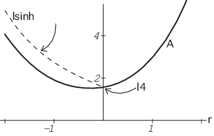
Figure 3 illustrates the diffierence between the upper bound (1.12) and the sharp asymptotic in this situation. Given this discrepancy, one might think that the bound in Theorem 1.4 could be improved by moving the boundary of KK further into the interior of the surface (i.e. by allowing bj<0b_{j}<0 in the definition (1.5)). Unfortunately, for reasons that we will explain in §4, it does not seem possible to obtain any improvement this way.

Refer to caption
Figure 3. The exact asymptotic constant for Fℓ,rF_{\ell,r} as a function of boundary location rr, shown for ℓ=2​π\ell=2\pi. The dotted line shows the bound from Theorem 1.4.

In the hyperbolic planar case, the model problem for YjY_{j} is scattering by a spherical obstacle in ℍ2\mathbb{H}^{2}, i.e. on the exterior Dirichlet domain Ωr0:={r≥r0}⊂ℍ2\Omega_{r_{0}}:=\{r\geq r_{0}\}\subset\mathbb{H}^{2}. The resonance asymptotics for this spherical obstacles in ℍn+1\mathbb{H}^{n+1} were worked out in Borthwick [4, Thm. 1.2]. In two dimensions the result is

(1.13) A⁡(Ωr0)=2−cosh⁡r0+4π​∫0π2∫0∞[H⁡(x​ei​θ,r0)]+x3​𝑑x​𝑑θ,A(\Omega_{r_{0}})=2-\cosh r_{0}+\frac{4}{\pi}\int_{0}^{\frac{\pi}{2}}\int_{0}^{\infty}\frac{[H(xe^{i\theta},r_{0})]_{+}}{x^{3}}\>dx\>d\theta,

where

(1.14) H⁡(α,r):=Re⁡[2​α​log⁡(α​cosh⁡r+1+α2​sinh2⁡rα2−1)]+log⁡|cosh⁡r−1+α2​sinh2⁡rcosh⁡r+1+α2​sinh2⁡r|.\begin{split}H(\alpha,r)&:=\operatorname{Re}\left[2\alpha\log\left(\frac{\alpha\cosh r+\sqrt{1+\alpha^{2}\sinh^{2}r}}{\sqrt{\alpha^{2}-1}}\right)\right]\\ &\qquad+\log\left|\frac{\cosh r-\sqrt{1+\alpha^{2}\sinh^{2}r}}{\cosh r+\sqrt{1+\alpha^{2}\sinh^{2}r}}\right|.\end{split}

The paper is organized as follows. The basic material on the resolvent and resonances of the operator PP is reviewed in §2. In §3 we present the factorization formula for the relative scattering determinant and show that this leads to Weyl asymptotics for the scattering phase and a counting formula for resonances based on contour integration. The growth estimates on the scattering determinant and the resulting proof of Theorem 1.4 are given in §4, assuming certain estimates to be developed in later sections. The derivation of Corollary 1.2 is also given in §4. In §5, we develop the asymptotic analysis of Dirichlet eigenmodes on hyperbolic funnels. These asymptotics are applied in §6 to prove the Poisson operator estimates needed for §4. Finally, in §7 and §8 we establish the exact asymptotic constant (1.10) for the truncated and extended funnel cases, respectively, establishing the funnel part of Theorem 1.3 in particular.

Acknowledgment. I would like to thank to Plamen Stefanov for suggesting the extension of his results to the hyperbolic setting. I am also grateful for support from the Banff International Research Station, where some of the work for this project was done.

2. Resonances

The context introduced in §1 differs from that of Guillopé-Zworski [8, 9] in two relatively minor ways: hyperbolic planar ends are allowed in addition to funnels, and a compactly supported potential VV is possibly added to Δg\Delta_{g}. The latter addition really is trivial, but the inclusion of hyperbolic planar ends requires a few extra estimates on model terms. In this section we will briefly review the theory [8, 9], in order to explain those additional estimates.

First of all, to define resonances we need analytic continuation of the resolvent, RP​(s):=(P−s⁡(1−s))−1R_{P}(s):=(P-s(1-s))^{-1} from its original domain Re⁡s>12\operatorname{Re}s>\tfrac{1}{2}. Each end YjY_{j} is isometric to a portion of either ℍ\mathbb{H} or the model funnel FℓjF_{\ell_{j}}, and we can use this identification to pullback model resolvents RYj0​(s)R^{0}_{Y_{j}}(s). After appropriate cutoffs are applied, we can treat these model terms as operators on XX, whose kernels have support only in the corresponding ends YjY_{j}. Similarly, we define RCj0​(s)R^{0}_{C_{j}}(s) by pullback from the model cusp. Suppose that χkj∈C∞​(X)\chi^{j}_{k}\in C^{\infty}(X) are cutoff functions for j=1,…,nf+ncj=1,\dots,{n_{\rm f}}+{n_{\rm c}} and k=0,1,2k=0,1,2, such that

χkj={0for ​r≥k+1​ in end ​j,1for ​r≤k​ in end ​j,1 outside of end ​j.\chi^{j}_{k}=\begin{cases}0&\text{for }r\geq k+1\text{ in end }j,\\ 1&\text{for }r\leq k\text{ in end }j,\\ 1&\text{ outside of end }j.\end{cases}

We also set χk:=∏jχkj\chi_{k}:=\prod_{j}\chi^{j}_{k}.

For some s0s_{0} with Re⁡s0\operatorname{Re}s_{0} sufficiently large, so that RP​(s0)R_{P}(s_{0}) is defined, we set

M⁡(s):=χ2​RP​(s0)​χ1+∑j=1nf(1−χ0j)​RYj0​(s)​(1−χ1j)+∑j=nf+1nf+nc(1−χ0j)​RCj0​(s)​(1−χ1j).M(s):=\chi_{2}R_{P}(s_{0})\chi_{1}+\sum_{j=1}^{n_{\rm f}}(1-\chi^{j}_{0})R^{0}_{Y_{j}}(s)(1-\chi^{j}_{1})+\sum_{j={n_{\rm f}}+1}^{{n_{\rm f}}+{n_{\rm c}}}(1-\chi^{j}_{0})R^{0}_{C_{j}}(s)(1-\chi^{j}_{1}).

This parametrix satisfies

(P−s⁡(1−s))​M​(s)=I−L⁡(s),(P-s(1-s))M(s)=I-L(s),

where

L⁡(s):=−[Δg,χ2]​RP​(s0)​χ1+(s⁡(1−s)−s0​(1−s0))​χ2​RP​(s0)​χ1+∑j=1nf[Δg,χj0]R0Yj(s)(1−χj1)+∑j=nf+1nf+nc[Δg,χj0]R0Cj(s)(1−χj1).\begin{split}L(s)&:=-[\Delta_{g},\chi_{2}]R_{P}(s_{0})\chi_{1}+(s(1-s)-s_{0}(1-s_{0}))\chi_{2}R_{P}(s_{0})\chi_{1}\\ &\qquad+\sum_{j=1}^{n_{\rm f}}[\Delta_{g},\chi^{j}_{0}]R^{0}_{Y_{j}}(s)(1-\chi^{j}_{1})+\sum_{j={n_{\rm f}}+1}^{{n_{\rm f}}+{n_{\rm c}}}[\Delta_{g},\chi^{j}_{0}]R^{0}_{C_{j}}(s)(1-\chi^{j}_{1}).\end{split}

The are two differences here from the construction of [8]. First of all, some of our model terms RYj0​(s)R^{0}_{Y_{j}}(s) will be copies of Rℍ​(s)R_{\mathbb{H}}(s) instead of the funnel resolvent. Second, we follow the treatment in Borthwick [2] in using the model resolvent for a full cusp, rather than modifying the original Hilbert space.

Let ρ∈C∞​(X)\rho\in C^{\infty}(X) be proportional to e−re^{-r} in the ends YjY_{j} and CjC_{j}, with respect to the coordinate systems given in (1.4–1.6). The operator L⁡(s)L(s) is compact on ρN​L2​(X,d​g)\rho^{N}L^{2}(X,dg) for Re⁡s>12−N\operatorname{Re}s>\tfrac{1}{2}-N and defines a meromorphic family with poles of finite rank. (The structure of the kernel of RYj0​(s)R^{0}_{Y_{j}}(s) at infinity is the same whether YjY_{j} is a funnel or hyperbolic planar, so this part of the argument is unaffected by the addition of hyperbolic planar ends.)

By choosing ss and s0s_{0} appropriately we can insure that I−L⁡(s)I-L(s) is invertible at some ss, and then the analytic Fredholm yields

(2.1) RP​(s)=M⁡(s)​(I−L⁡(s))−1.R_{P}(s)=M(s)(I-L(s))^{-1}.

This proves the following result, a slight generalization of [8, Thm. 1]:

Theorem 2.1 (Guillopé-Zworski).

The formula (2.1) defines a meromorphic extension of RP​(s)R_{P}(s) to a bounded operator on ρN​L2​(X,d​g)\rho^{N}L^{2}(X,dg) for Re⁡s>12−N\operatorname{Re}s>\tfrac{1}{2}-N, with poles of finite rank.

Meromorphic continuation allows us to define ℛP\mathcal{R}_{P} as the set of poles of RP​(s)R_{P}(s), listed according to multiplicities given by

mP​(ζ):=rank⁡Resζ​RP​(s).m_{P}(\zeta):=\operatorname{rank}\operatorname{Res}_{\zeta}R_{P}(s).

The same parametrix construction also leads to an estimate of the order of growth of the resonance counting function. The following is a slight generalization of [8, Thm 2]:

Theorem 2.2 (Guillopé-Zworski).

The resonance counting function satisfies a bound

NP​(t)=O⁡(t2).N_{P}(t)=O(t^{2}).

Our version requires just a few additional estimates. To obtain this bound on the counting function, Guillopé-Zworski [8] introduced a Fredholm determinant

D⁡(s):=det(I−L3​(s)3),D(s):=\det(I-L_{3}(s)^{3}),

where

L3​(s):=L⁡(s)​χ3.L_{3}(s):=L(s)\chi_{3}.

Using the relation

RP​(s)​χ3=M⁡(s)​χ3​(I+L3​(s)+L3​(s)2)​(I−L3​(s)3)−1,R_{P}(s)\chi_{3}=M(s)\chi_{3}(I+L_{3}(s)+L_{3}(s)^{2})(I-L_{3}(s)^{3})^{-1},

and a result of Vodev [16, Appendix], they showed that ℛP\mathcal{R}_{P} is included in the union of the set of poles of D⁡(s)D(s) with 3 copies of the union of the sets of poles of M⁡(s)M(s) and L3​(s)L_{3}(s).

The only change that the inclusion of hyperbolic planar ends requires in this argument is that for each hyperbolic planar end we include a copy of ℛℍ\mathcal{R}_{\mathbb{H}} among the possible poles of M⁡(s)M(s) and L3​(s)L_{3}(s). Since Nℍ​(t)=O⁡(t2)N_{\mathbb{H}}(t)=O(t^{2}), just as for funnels, the problem reduces as in [8] to an estimate of the growth of D⁡(s)D(s). Through Weyl’s inequality, the estimate of D⁡(s)D(s) is broken up into estimates on the singular values of various model terms. We must check that the relevant estimates are satisfied by the hyperbolic planar model terms.

There are three estimates to consider. The first concerns the resolvent Rℍ​(s)R_{\mathbb{H}}(s). If Q1,Q2Q_{1},Q_{2} are compactly supported differential operators of orders q1,q2q_{1},q_{2}, with disjoint supports, then for ε>0\varepsilon>0,

(2.2) ‖Q1​Rℍ​(s)​Q2‖≤C⁡(qj,ε)​⟨s⟩q1+q2,for ​Re⁡s>ε,\|Q_{1}R_{\mathbb{H}}(s)Q_{2}\|\leq C(q_{j},\varepsilon)\>\langle s\rangle^{q_{1}+q_{2}},\quad\text{for }\operatorname{Re}s>\varepsilon,

and

(2.3) ‖Q1​Rℍ​(s)​Q2‖≤C⁡(qj,ε)​⟨s⟩q1+q2−1,for ​Re⁡s>12+ε.\|Q_{1}R_{\mathbb{H}}(s)Q_{2}\|\leq C(q_{j},\varepsilon)\>\langle s\rangle^{q_{1}+q_{2}-1},\quad\text{for }\operatorname{Re}s>\tfrac{1}{2}+\varepsilon.

To prove either of these, one can simply use the explicit formula,

Rℍ​(s,z,z′)=14​π​∫01(t⁡(1−t))s−1[t+sinh2⁡d⁡(z,z′)]s​𝑑t,R_{\mathbb{H}}(s;z,z^{\prime})=\frac{1}{4\pi}\int_{0}^{1}\frac{(t(1-t))^{s-1}}{[t+\sinh^{2}d(z,z^{\prime})]^{s}}\>dt,

and repeat the argument from [8, Lemma 3.2].

The next estimate is for the Poisson kernel Eℍ​(s)E_{\mathbb{H}}(s). In the Poincaré ball model 𝔹\mathbb{B}, this kernel is given by

E𝔹​(s,z,θ)=14​π​Γ​(s)2Γ⁡(2​s)​(1−|z|2)s|ei​θ−z|2​s,z∈𝔹,θ∈ℝ/(2​π​ℤ).E_{\mathbb{B}}(s;z,\theta)=\frac{1}{4\pi}\frac{\Gamma(s)^{2}}{\Gamma(2s)}\frac{(1-|z|^{2})^{s}}{|e^{i\theta}-z|^{2s}},\qquad z\in\mathbb{B},\>\theta\in\mathbb{R}/(2\pi\mathbb{Z}).

Given a compact set K⊂𝔹K\subset\mathbb{B} and ε>0\varepsilon>0, we have

(2.4) |∂θkE𝔹​(s,z,θ)|≤C​(K,ε)k​k!​ec​⟨s⟩,for ​z∈K,k∈ℕ.\bigl|\partial^{k}_{\theta}E_{\mathbb{B}}(s;z,\theta)\bigr|\leq C(K,\varepsilon)^{k}\>k!\>e^{c\langle s\rangle},\quad\text{for }z\in K,\>k\in\mathbb{N}.

This is not difficult to prove directly by induction, or one can use an analyticity argument as in [8, Lemma 3.1].

Finally, we must estimate the scattering matrix Sℍ​(s)S_{\mathbb{H}}(s). We can write this explicitly in terms of Fourier modes,

Sℍ​(s)=∑k∈ℤ[Sℍ​(s)]k​ei​k​(θ−θ′),S_{\mathbb{H}}(s)=\sum_{k\in\mathbb{Z}}[S_{\mathbb{H}}(s)]_{k}e^{ik(\theta-\theta^{\prime})},

where

[Sℍ​(s)]k=21−2​s​Γ⁡(12−s)Γ⁡(s−12)​Γ⁡(s+|k|)Γ⁡(1−s+|k|)[S_{\mathbb{H}}(s)]_{k}=2^{1-2s}\frac{\Gamma(\tfrac{1}{2}-s)}{\Gamma(s-\tfrac{1}{2})}\frac{\Gamma(s+|k|)}{\Gamma(1-s+|k|)}

Using Stirling’s formula, it is easy to use this expression for the eigenvalues to estimate the singular values of Sℍ​(s)S_{\mathbb{H}}(s). Assuming that Re⁡s<12−ε\operatorname{Re}s<\tfrac{1}{2}-\varepsilon and dist⁡(s,−ℕ0)>η\operatorname{dist}(s,-\mathbb{N}_{0})>\eta, we have

(2.5) μj​(Sℍ​(s))≤exp⁡[C⁡(η)​⟨s⟩+Re⁡(1−2​s)​log⁡⟨s⟩j].\mu_{j}(S_{\mathbb{H}}(s))\leq\exp\left[C(\eta)\>\langle s\rangle+\operatorname{Re}(1-2s)\log\frac{\langle s\rangle}{j}\right].

This is the analog of [9, Lemma 4.2].

With these model estimates in place, one can simply apply Guillopé-Zworski’s original argument (treating the cusp contributions as in [2, §9.4]) to prove that

|g⁡(s)​D​(s)|≤eC​⟨s⟩2,|g(s)D(s)|\leq e^{C\langle s\rangle^{2}},

where g⁡(s)g(s) is a entire function of order 2 and finite type, with zeros derived from ℛℍ\mathcal{R}_{\mathbb{H}} and the the model resolvent sets for the funnels and cusps. This yields the proof of Theorem 2.2.

3. Relative scattering determinant

To define scattering matrices, we will fix a function ρ∈C∞​(X)\rho\in C^{\infty}(X) which serves as a boundary defining function for a suitable compactification of XX. We start with smooth positive functions ρf\rho_{\rm f}, ρc\rho_{\rm c} satisfying

ρf={2​e−rin each ​Yj,1in each ​Cj,ρc={1in each ​Yj,e−rin each ​Cj.\rho_{\rm f}=\begin{cases}2e^{-r}&\text{in each }Y_{j},\\ 1&\text{in each }C_{j},\end{cases}\qquad\rho_{\rm c}=\begin{cases}1&\text{in each }Y_{j},\\ e^{-r}&\text{in each }C_{j}.\end{cases}

Then we set ρ=ρf​ρc\rho=\rho_{\rm f}\rho_{\rm c} for the global boundary defining function.

The ends YjY_{j} are conformally compact, and we distinguish between the internal boundary ∂Yj\partial Y_{j}, and the boundary at infinity ∂∞Yj\partial_{\infty}Y_{j} induced by the conformal compactification. The funnel ends YjY_{j} come equipped with a length parameter ℓj\ell_{j}, the length of the closed geodesic bounding the finite end. If we assign length ℓj=2​π\ell_{j}=2\pi to a hyperbolic planar end, for consistency, then the metric induced by ρ2​g\rho^{2}g on the boundary of YjY_{j} at infinity gives an isometry

∂∞Yj≅ℝ/ℓj​ℤ.\partial_{\infty}Y_{j}\cong\mathbb{R}/\ell_{j}\mathbb{Z}.

The cusp ends can be compactified naturally by lifting to ℍ\mathbb{H} and invoking the Riemann-sphere topology, as described in [2, §6.1]. The resulting boundary ∂∞Cj\partial_{\infty}C_{j} consists of a single point.

Despite the discrepancy in dimensions, it will be convenient to group all of the infinite boundaries together as

∂∞X:=∂∞Y1∪⋯∪∂∞Ynf∪∂∞Cnf+1∪⋯∪∂∞Cnf+nc.\partial_{\infty}X:=\partial_{\infty}Y_{1}\cup\dots\cup\partial_{\infty}Y_{{n_{\rm f}}}\cup\partial_{\infty}C_{{n_{\rm f}}+1}\cup\dots\cup\partial_{\infty}C_{{n_{\rm f}}+{n_{\rm c}}}.

Then we have

C∞​(∂∞X):=C∞​(ℝ/ℓ1​ℤ)⊕⋯⊕C∞​(ℝ/ℓnf​ℤ)⊕ℂnc,C^{\infty}(\partial_{\infty}X):=C^{\infty}(\mathbb{R}/\ell_{1}\mathbb{Z})\oplus\dots\oplus C^{\infty}(\mathbb{R}/\ell_{{n_{\rm f}}}\mathbb{Z})\oplus\mathbb{C}^{{n_{\rm c}}},

and similarly for L2​(∂∞X)L^{2}(\partial_{\infty}X).

In §2, RYj0​(s)R^{0}_{Y_{j}}(s) denoted the pullback of the model resolvent in the parametrix construction. Carrying on with this notation, we also define the model Poisson operators,

EYj0​(s):C∞​(∂∞Yj)→L2​(Yj),E^{0}_{Y_{j}}(s):C^{\infty}(\partial_{\infty}Y_{j})\to L^{2}(Y_{j}),

and scattering matrices,

SYj0​(s):C∞​(∂∞Yj)→C∞​(∂∞Yj).S^{0}_{Y_{j}}(s):C^{\infty}(\partial_{\infty}Y_{j})\to C^{\infty}(\partial_{\infty}Y_{j}).

Similarly, for the cusp ends we have the Poisson kernels

ECj0​(s):ℂ→L2​(Cj).E^{0}_{C_{j}}(s):\mathbb{C}\to L^{2}(C_{j}).

There is no analog of the model scattering matrix for a cusp; see [2, §7.5] for an explanation of this.

The scattering matrix SP​(s)S_{P}(s) is defined as a map on C∞​(∂∞X)C^{\infty}(\partial_{\infty}X), which we can write as

(3.1) SP​(s)=(Sff​(s)Sfc​(s)Scf​(s)Scc​(s)),S_{P}(s)=\begin{pmatrix}S^{\rm ff}(s)&S^{\rm fc}(s)\\ S^{\rm cf}(s)&S^{\rm cc}(s)\end{pmatrix},

where the blocks are split between the ‘funnel-type’ ends YjY_{j} and the cusps CjC_{j}. The block Sff​(s)S^{\rm ff}(s) is a matrix of pseudodifferential operators; all other blocks have finite rank. To define a scattering determinant, we normalize using the background operator

S0​(s)=(SY0​(s)00I),S_{0}(s)=\begin{pmatrix}S^{0}_{Y}(s)&0\\ 0&I\end{pmatrix},

where

SY0​(s)=SY10​(s)⊕⋯⊕SYnf0​(s).S^{0}_{Y}(s)=S^{0}_{Y_{1}}(s)\oplus\dots\oplus S^{0}_{Y_{{n_{\rm f}}}}(s).

The relative scattering determinant is then defined by

(3.2) τ⁡(s)=detSP​(s)​S0​(s)−1.\tau(s)=\det S_{P}(s)S_{0}(s)^{-1}.

The poles of the background scattering matrix S0​(s)S_{0}(s) define a background resonance set

(3.3) ℛ0=⋃j=1nf{ℛFℓjfor a funnel end,ℛℍfor a hyperbolic planar end.\mathcal{R}_{0}=\bigcup_{j=1}^{n_{\rm f}}\begin{cases}\mathcal{R}_{F_{\ell_{j}}}&\text{for a funnel end,}\\ \mathcal{R}_{\mathbb{H}}&\text{for a hyperbolic planar end.}\end{cases}

For ∗=0*=0 or PP let H∗​(s)H_{*}(s) denote the Hadamard product over ℛ∗\mathcal{R}_{*},

H∗​(s):=∏ζ∈ℛ∗(1−sζ)​esζ+s22​ζ2.H_{*}(s):=\prod_{\zeta\in\mathcal{R}_{*}}\left(1-\frac{s}{\zeta}\right)e^{\frac{s}{\zeta}+\frac{s^{2}}{2\zeta^{2}}}.

Theorem 2.2 implies that the product for HP​(s)H_{P}(s) converges, and for H0​(s)H_{0}(s) this is clear from the definition of ℛ0\mathcal{R}_{0}.

Proposition 3.1.

For P=Δg+VP=\Delta_{g}+V, the relative scattering determinant admits a factorization

τ⁡(s)=eq⁡(s)​HP​(1−s)HP​(s)​H0​(s)H0​(1−s),\tau(s)=e^{q(s)}\frac{H_{P}(1-s)}{H_{P}(s)}\frac{H_{0}(s)}{H_{0}(1-s)},

where q⁡(s)q(s) is a polynomial of degree at most 2.

Proof.

If the ends YjY_{j} are all hyperbolic funnels, then Guillopé-Zworski [9, Prop. 3.7] proved the factorization formula of with q⁡(s)q(s) a polynomial of degree at most 4. The first part of the proof, the characterization of the divisor of τ⁡(s)\tau(s) obtained in [9, Prop. 2.14], remains valid if hyperbolic planar ends are included.

To extend the more difficult part of the argument, which is the estimate that shows q⁡(s)q(s) is polynomial, we require only the extra estimates on model terms given in (2.2), (2.3), (2.4), and (2.5). With these estimates one can easily extend the proof of [9, Prop. 3.7]. We refer the reader also to [2, §10.5], for an expository treatment of these details.

To see that the maximal order of q⁡(s)q(s) is 2, we could prove an estimate analogous to [3, Lemma 5.2]. However, we will be proving a sharper version of this estimate later in this paper. From the proof of Theorem 4.1, it will follow that for some sequence ai→∞a_{i}\to\infty,

log⁡|τ⁡(s)|≤O⁡(ai2)for ​|s−12|=ai,Re⁡s≥12.\log|\tau(s)|\leq O(a_{i}^{2})\quad\text{for }|s-\tfrac{1}{2}|=a_{i},\>\operatorname{Re}s\geq\tfrac{1}{2}.

Because the Hadamard products H∗​(s)H_{*}(s) have order 2, this implies a bound |q⁡(s)|=O⁡(|s|2+ε)|q(s)|=O(|s|^{2+\varepsilon}) for Re⁡s≥12\operatorname{Re}s\geq\tfrac{1}{2}. This implies q⁡(s)q(s) has degree at most 2, since it is already known to be polynomial. (The derivations leading to Theorem 4.1 require only that q⁡(s)q(s) is polynomial, so this argument is not circular.) ∎

To apply the factorization of τ⁡(s)\tau(s) to resonance counting we introduce the relative scattering phase of PP, defined as

(3.4) σ⁡(ξ):=i2​π​log⁡τ⁡(12+i​ξ),\sigma(\xi):=\frac{i}{2\pi}\log\tau(\tfrac{1}{2}+i\xi),

with branches of the log chosen so that σ⁡(ξ)\sigma(\xi) is continuous and σ⁡(0)=0\sigma(0)=0. By the properties of the relative scattering matrix, σ⁡(ξ)\sigma(\xi) is real and σ⁡(−ξ)=−σ⁡(ξ)\sigma(-\xi)=-\sigma(\xi).

To state the relative counting formula, we let N0N_{0} denote the counting function associated to ℛ0\mathcal{R}_{0},

N0​(t):=#⁡{ζ∈ℛ0:|ζ−12|≤t},N_{0}(t):=\#\bigl\{\zeta\in\mathcal{R}_{0}:\>|\zeta-\tfrac{1}{2}|\leq t\bigr\},

and N~0​(a)\widetilde{N}_{0}(a) the corresponding regularized counting function.

Corollary 3.2.

As a→∞a\to\infty,

(3.5) N~P​(a)−N~0​(a)=4​∫0aσ⁡(t)t​𝑑t+2π​∫0π2log|τ⁡(12+a​ei​θ)|𝑑θ+O⁡(log⁡a).\widetilde{N}_{P}(a)-\widetilde{N}_{0}(a)=4\int_{0}^{a}\frac{\sigma(t)}{t}\>dt+\frac{2}{\pi}\int_{0}^{\frac{\pi}{2}}\log|\tau(\tfrac{1}{2}+ae^{i\theta})|\>d\theta+O(\log a).

The proof is by contour integration of τ′/τ⁡(s)\tau^{\prime}/\tau(s) around a half-circle centered at s=12s=\tfrac{1}{2}. See [4, Prop. 3.2] for the details of the derivation of (3.5) from Proposition 3.1. This is the analog of a formula developed by Froese [6] for Schrödinger operators in the Euclidean setting.

The other consequence we need from Proposition 3.1 is essentially also already proven. To analyze the first term on the right-hand side of (3.5), we will invoke the Weyl-type asymptotics satisfied by the scattering phase:

Theorem 3.3 (Guillopé-Zworski).

As ξ→+∞\xi\to+\infty,

σ⁡(ξ)=(14​π​0−vol⁡(X,g)−nhp2)​ξ2−ncπ​ξ​log⁡ξ+O⁡(ξ),\sigma(\xi)=\left(\frac{1}{4\pi}\operatorname{0-vol}(X,g)-\frac{n_{\rm hp}}{2}\right)\>\xi^{2}-\frac{{n_{\rm c}}}{\pi}\xi\log\xi+O(\xi),

where nhpn_{\rm hp} denotes the number of YjY_{j}’s that are hyperbolic planar.

For surfaces with hyperbolic funnel or cusp ends this result was established in Guillopé-Zworski [9, Thm. 1.5]. As in the other cases discussed above, the modifications needed to adapt the proof to our slightly more general setting are fairly simple. The first point is that the addition of a compactly supported potential VV does not change the argument at all, since it does not affect the leading term in the wave trace asymptotics as derived in [9, Lemma 6.2]. The second issue is that we allow hyperbolic planar ends in addition to funnels. However, for |t|<ℓ|t|<\ell the restriction to the diagonal of the wave kernel on a model funnel FℓF_{\ell} is identical to that of ℍ2\mathbb{H}^{2}. This is the content of [9, eq. (6.1)]. So hyperbolic planar ends may also be included without modifying the argument. Such ends do affect the final calculation, however, because 0−vol⁡(ℍ2)=−2​π\operatorname{0-vol}(\mathbb{H}^{2})=-2\pi whereas the model funnels had 0−vol⁡(Fℓ)=0\operatorname{0-vol}(F_{\ell})=0. This difference accounts for the nhpn_{\rm hp} term.

4. Scattering determinant asymptotics

To state the asymptotic estimate for the scattering determinant contribution to the resonance counting formula (3.5), we introduce the following constants. If YjY_{j} is a funnel with parameters ℓj,bj\ell_{j},b_{j}, then we set

B⁡(Yj):=4π​∫0π2∫0∞[I⁡(x​ei​θ,ℓj,bj)]+x3​𝑑x​𝑑θ−ℓj4,B(Y_{j}):=\frac{4}{\pi}\int_{0}^{\frac{\pi}{2}}\int_{0}^{\infty}\frac{[I(xe^{i\theta},\ell_{j},b_{j})]_{+}}{x^{3}}\>dx\>d\theta-\frac{\ell_{j}}{4},

where I⁡(α,ℓ,r)I(\alpha,\ell,r) was defined in (1.11). If YjY_{j} is a hyperbolic planar end with parameter bjb_{j}, then

B⁡(Yj):=4π​∫0π2∫0∞[H⁡(x​ei​θ,bj)]+x3​𝑑x​𝑑θ,B(Y_{j}):=\frac{4}{\pi}\int_{0}^{\frac{\pi}{2}}\int_{0}^{\infty}\frac{[H(xe^{i\theta},b_{j})]_{+}}{x^{3}}\>dx\>d\theta,

where H⁡(α,ℓ,r)H(\alpha,\ell,r) was defined in (1.14). The cusps do not contribute to the asymptotics of τ⁡(s)\tau(s) to leading order, so we make no analogous definition for CjC_{j}.

Theorem 4.1.

For (X,g)(X,g) a surface with hyperbolic ends as in (1.3), there exists an unbounded set Λ⊂[1,∞)\Lambda\subset[1,\infty) such that

2π​∫0π2log|τ⁡(12+a​ei​θ)|𝑑θ≤∑j=1nfB⁡(Yj)​a2+o⁡(a2)\frac{2}{\pi}\int_{0}^{\frac{\pi}{2}}\log|\tau(\tfrac{1}{2}+ae^{i\theta})|\>d\theta\leq\sum_{j=1}^{n_{\rm f}}B(Y_{j})a^{2}+o(a^{2})

for all a∈Λa\in\Lambda.

Before undertaking the proof of Theorem 4.1, we will show how this theorem leads to the proof of the main result stated in §1:

Proof of Theorem 1.4.

Starting from the counting formula from Corollary 3.2, we apply Theorem 3.3 to the scattering phase term and Theorem 4.1 to the scattering determinant contribution. This yields

(4.1) N~P​(a)≤N~0​(a)+12​π​0−vol⁡(X,g)​a2+∑j=1nfB⁡(Yj)​a2+o⁡(a2),\widetilde{N}_{P}(a)\leq\widetilde{N}_{0}(a)+\frac{1}{2\pi}\operatorname{0-vol}(X,g)a^{2}+\sum_{j=1}^{n_{\rm f}}B(Y_{j})a^{2}+o(a^{2}),

as a→∞a\to\infty. From the explicit definition (3.3) of ℛ0\mathcal{R}_{0}, we see that

N0​(t)t2∼∑j=1nf{1for a hyperbolic planar end,ℓj4for a funnel end,\frac{N_{0}(t)}{t^{2}}\sim\sum_{j=1}^{n_{\rm f}}\begin{cases}1&\text{for a hyperbolic planar end,}\\ \frac{\ell_{j}}{4}&\text{for a funnel end,}\end{cases}

and so N~0​(a)\widetilde{N}_{0}(a) satisfies the same asymptotic. Also, we have

0−vol⁡(X,g)=vol⁡(Xc,g)+∑j=1nf0−vol⁡(Yj,g).\operatorname{0-vol}(X,g)=\operatorname{vol}(X_{\rm c},g)+\sum_{j=1}^{{n_{\rm f}}}\operatorname{0-vol}(Y_{j},g).

The 00-volumes of the YjY_{j}’s are easily computed. For a hyperbolic planar end,

0−vol(Yj,g)=2πFPε→0∫bjlog⁡(2/ε)sinhrdr=−2πcoshbj,\operatorname{0-vol}(Y_{j},g)=2\pi\operatornamewithlimits{FP}_{\varepsilon\to 0}\int_{b_{j}}^{\log(2/\varepsilon)}\sinh r\>dr=-2\pi\cosh b_{j},

and for a funnel end,

0−vol(Yj,g)=ℓjFPε→0∫bjlog⁡(2/ε)coshrdr=−ℓjsinhbj.\operatorname{0-vol}(Y_{j},g)=\ell_{j}\operatornamewithlimits{FP}_{\varepsilon\to 0}\int_{b_{j}}^{\log(2/\varepsilon)}\cosh r\>dr=-\ell_{j}\sinh b_{j}.

By the formulas (1.13) and (1.10) for A⁡(Yj)A(Y_{j}), we then see that (4.1) is equivalent to the claimed estimate. ∎

The derivation of Theorem 1.1 from Theorem 1.4 was already explained in §1. To prove Corollary 1.2 we simply recall a few details of the proof of the lower bound in Guillopé-Zworski [9, Thm. 1.3]. For a test function ϕ∈C0∞​(ℝ+)\phi\in C^{\infty}_{0}(\mathbb{R}_{+}) with ϕ≥0\phi\geq 0 and ϕ⁡(1)>0\phi(1)>0, we have estimates

|ϕ^​(ξ)|≤Ck​(1+|ξ|)−k−2,|\hat{\phi}(\xi)|\leq C_{k}(1+|\xi|)^{-k-2},

for k∈ℕk\in\mathbb{N} and Im⁡ξ≤0\operatorname{Im}\xi\leq 0. Pairing the distributional Poisson formula [9, Thm. 5.7] with λϕ(λ⋅)\lambda\phi(\lambda\,\cdot) yields

|0−vol⁡(X,g)|​λ2≤Ck​∫0∞(1+r)−k−3​NP​(λ​r)​𝑑r.|\operatorname{0-vol}(X,g)|\>\lambda^{2}\leq C_{k}\int_{0}^{\infty}(1+r)^{-k-3}N_{P}(\lambda r)\>dr.

If we have NP​(t)≤A​t2N_{P}(t)\leq At^{2} for t≥1t\geq 1, then splitting the integral at aa gives

|0−vol⁡(X,g)|​λ2≤Ck​[N⁡(λ​a)+A​λ2​a−k].|\operatorname{0-vol}(X,g)|\>\lambda^{2}\leq C_{k}\Bigl[N(\lambda a)+A\lambda^{2}a^{-k}\Bigr].

Setting t=λ​at=\lambda a, we have

N⁡(t)≥(ck​|0−vol⁡(X,g)|​a−2−A​a−2−k)​t2,N(t)\geq\Bigl(c_{k}\>|\operatorname{0-vol}(X,g)|\>a^{-2}-Aa^{-2-k}\Bigr)\>t^{2},

and optimizing with respect to aa then yields

N(t)≥ck|0−vol(X,g)|1+k/2A−k/2.N(t)\geq c_{k}\>|\operatorname{0-vol}(X,g)|^{1+k/2}A^{-k/2}.

Corollary 1.2 is then proven by substituting the constant obtained in Theorem 1.1 for AA.

The rest of this section is devoted to the proof of Theorem 4.1. To produce a formula convenient for estimation, we introduce cutoff functions as follows. Fix some η∈(0,1)\eta\in(0,1). For j=1,…,nf+ncj=1,\dots,{n_{\rm f}}+{n_{\rm c}} and k=1,2k=1,2, we define χkj∈C∞​(X)\chi^{j}_{k}\in C^{\infty}(X) so that χkj=1\chi^{j}_{k}=1 outside the jj-th end (YjY_{j} or CjC_{j}), and inside the jj-th end we have

(4.2) χkj={0for ​r≥bj+(k+1)​η,1for ​r≤bj+k​η.\chi^{j}_{k}=\begin{cases}0&\text{for }r\geq b_{j}+(k+1)\eta,\\ 1&\text{for }r\leq b_{j}+k\eta.\end{cases}
Refer to caption
Figure 4. The cutoff functions χkj\chi^{j}_{k} in the jj-th end.
Proposition 4.2.

With cutoffs defined as in (4.2), we have

SX​(s)​S0​(s)−1=I+Q⁡(s),S_{X}(s)S_{0}(s)^{-1}=I+Q(s),

where the components of Q⁡(s)Q(s), in terms of the block decomposition introduced in (3.1), are

Qi​jff​(s)=(2​s−1)​EYi0​(s)t​[ΔYi,χ2i]​RP​(s)​[ΔYj,χ1j]​EYj0​(1−s),Q^{\rm ff}_{ij}(s)=(2s-1)E^{0}_{Y_{i}}(s)^{t}[\Delta_{Y_{i}},\chi^{i}_{2}]R_{P}(s)[\Delta_{Y_{j}},\chi^{j}_{1}]E^{0}_{Y_{j}}(1-s),
Qi​jcf​(s)=(2​s−1)​ECi0​(s)t​[ΔCi,χ2i]​RP​(s)​[ΔYj,χ1j]​EYj0​(1−s),Q^{\rm cf}_{ij}(s)=(2s-1)E^{0}_{C_{i}}(s)^{t}[\Delta_{C_{i}},\chi^{i}_{2}]R_{P}(s)[\Delta_{Y_{j}},\chi^{j}_{1}]E^{0}_{Y_{j}}(1-s),
Qi​jfc​(s)=−(2​s−1)​EYi0​(s)t​[ΔYi,χ2i]​RP​(s)​[ΔCj,χ1j]​ECj0​(s),Q^{\rm fc}_{ij}(s)=-(2s-1)E^{0}_{Y_{i}}(s)^{t}[\Delta_{Y_{i}},\chi^{i}_{2}]R_{P}(s)[\Delta_{C_{j}},\chi^{j}_{1}]E^{0}_{C_{j}}(s),
Qi​jcf​(s)=−(2​s−1)​ECi0​(s)t​[ΔCi,χ2i]​RP​(s)​[ΔCj,χ1j]​ECj0​(s),Q^{\rm cf}_{ij}(s)=-(2s-1)E^{0}_{C_{i}}(s)^{t}[\Delta_{C_{i}},\chi^{i}_{2}]R_{P}(s)[\Delta_{C_{j}},\chi^{j}_{1}]E^{0}_{C_{j}}(s),
Proof.

We first note that one characterize the scattering matrix SX​(s)S_{X}(s) through the boundary behavior of solutions of (Δg−s⁡(1−s))​u=0(\Delta_{g}-s(1-s))u=0. For ψ∈C∞​(∂∞X)\psi\in C^{\infty}(\partial_{\infty}X) and Re⁡s≥12\operatorname{Re}s\geq\tfrac{1}{2}, s≠ℕ/2s\neq\mathbb{N}/2, there is a unique generalized eigenfunction u∈C∞​(X)u\in C^{\infty}(X) with the asymptotic behavior

(4.3) u∼ρf1−s​ρc−s​ψ+ρfs​ρcs−1​SX​(s)​ψ.u\sim\rho_{\rm f}^{1-s}\rho_{\rm c}^{-s}\psi+\rho_{\rm f}^{s}\rho_{\rm c}^{s-1}S_{X}(s)\psi.

For hyperbolic surfaces with cusps, a proof is given in Borthwick [2, Prop. 7.13]. The essential analysis takes place in the ends, so including smooth metric or potential perturbations within K0K_{0} requires only trivial modifications to the proof. Likewise, hyperbolic planar ends may be included without much change to the argument.

Suppose fj∈C∞​(∂∞Yj)f_{j}\in C^{\infty}(\partial_{\infty}Y_{j}). Then we can use the model Poisson kernel EYj0​(s)E^{0}_{Y_{j}}(s) to create a partial solution (1−χ1j)​EYj0​(s)​fj(1-\chi^{j}_{1})E^{0}_{Y_{j}}(s)f_{j} supported in YjY_{j}. As ρ→0\rho\to 0 in YjY_{j} this function has the asymptotic behavior

(4.4) (1−χ1j)​EYj0​(s)​fj∼12​s−1​[ρf1−s​fj+ρfs​SYj0​(s)​fj].(1-\chi^{j}_{1})E^{0}_{Y_{j}}(s)f_{j}\sim\frac{1}{2s-1}\Bigl[\rho_{\rm f}^{1-s}f_{j}+\rho_{\rm f}^{s}S^{0}_{Y_{j}}(s)f_{j}\Bigr].

To create a full solution will take the ansatz

u=(1−χ1j)​EYj0​(s)​fj+u′u=(1-\chi^{j}_{1})E^{0}_{Y_{j}}(s)f_{j}+u^{\prime}

and then solve (Δg−s⁡(1−s))​u=0(\Delta_{g}-s(1-s))u=0 for u′u^{\prime} by applying the resolvent. The result is

u′=RP​(s)​[ΔYj,χ1j]​EYj0​(s)​fj.u^{\prime}=R_{P}(s)[\Delta_{Y_{j}},\chi^{j}_{1}]E^{0}_{Y_{j}}(s)f_{j}.

In the end YiY_{i}, we can use the fact that (1−χ2i)​[ΔYj,χ1j]=0(1-\chi^{i}_{2})[\Delta_{Y_{j}},\chi^{j}_{1}]=0 to deduce

(ΔYi−s⁡(1−s))​(1−χ2i)​u′=−[ΔYi,χ2i]​u′,(\Delta_{Y_{i}}-s(1-s))(1-\chi^{i}_{2})u^{\prime}=-[\Delta_{Y_{i}},\chi^{i}_{2}]u^{\prime},

and hence that

(1−χ2i)​u′=−RYi0​(s)​[ΔYi,χ2i]​RP​(s)​[ΔYj,χ1j]​EYj0​(s)​fj.(1-\chi^{i}_{2})u^{\prime}=-R^{0}_{Y_{i}}(s)[\Delta_{Y_{i}},\chi^{i}_{2}]R_{P}(s)[\Delta_{Y_{j}},\chi^{j}_{1}]E^{0}_{Y_{j}}(s)f_{j}.

This gives the asymptotic behavior in YiY_{i}:

(4.5) u′∼−ρfs​EYi0​(s)t​[ΔYi,χ2i]​RP​(s)​[ΔYj,χ1j]​EYj0​(s)​fj.u^{\prime}\sim-\rho_{\rm f}^{s}E^{0}_{Y_{i}}(s)^{t}[\Delta_{Y_{i}},\chi^{i}_{2}]R_{P}(s)[\Delta_{Y_{j}},\chi^{j}_{1}]E^{0}_{Y_{j}}(s)f_{j}.

By comparing the asymptotics (4.4) and (4.5) to the general form (4.3), we see that

Si​jff​(s)=δi​j​SYj0​(s)−(2​s−1)​EYi0​(s)t​[ΔYi,χ2i]​RP​(s)​[ΔYj,χ1j]​EYj0​(s)S^{\rm ff}_{ij}(s)=\delta_{ij}S^{0}_{Y_{j}}(s)-(2s-1)E^{0}_{Y_{i}}(s)^{t}[\Delta_{Y_{i}},\chi^{i}_{2}]R_{P}(s)[\Delta_{Y_{j}},\chi^{j}_{1}]E^{0}_{Y_{j}}(s)

We then obtain Qi​jff​(s)Q^{\rm ff}_{ij}(s) by noting that

EYj0​(s)​SYj0​(s)−1=−EYj0​(1−s).E^{0}_{Y_{j}}(s)S^{0}_{Y_{j}}(s)^{-1}=-E^{0}_{Y_{j}}(1-s).

To find Qi​jcf​(s)Q^{\rm cf}_{ij}(s) we use the same setup starting from fj∈C∞​(∂∞Yj)f_{j}\in C^{\infty}(\partial_{\infty}Y_{j}), but then analyze u′u^{\prime} by restricting to the the cusp end CiC_{i}. This yields

(1−χ2i)​u′=−RCi0​(s)​[ΔCi,χ2i]​RP​(s)​[ΔYj,χ1j]​EYj0​(s)​fj.(1-\chi^{i}_{2})u^{\prime}=-R^{0}_{C_{i}}(s)[\Delta_{C_{i}},\chi^{i}_{2}]R_{P}(s)[\Delta_{Y_{j}},\chi^{j}_{1}]E^{0}_{Y_{j}}(s)f_{j}.

The asymptotic behavior in CiC_{i} is given by

(1−χ2i)​u′∼−ρs−1​ECi0​(s)t​[ΔCi,χ2i]​RP​(s)​[ΔYj,χ1j]​EYj0​(s)​fj,(1-\chi^{i}_{2})u^{\prime}\sim-\rho^{s-1}E^{0}_{C_{i}}(s)^{t}[\Delta_{C_{i}},\chi^{i}_{2}]R_{P}(s)[\Delta_{Y_{j}},\chi^{j}_{1}]E^{0}_{Y_{j}}(s)f_{j},

so that

Si​jcf​(s)=−(2​s−1)​ECi0​(s)t​[ΔCi,χ2i]​RP​(s)​[ΔYj,χ1j]​EYj0​(s).S^{\rm cf}_{ij}(s)=-(2s-1)E^{0}_{C_{i}}(s)^{t}[\Delta_{C_{i}},\chi^{i}_{2}]R_{P}(s)[\Delta_{Y_{j}},\chi^{j}_{1}]E^{0}_{Y_{j}}(s).

Next take aj∈C∞​(∂∞Cj)=ℂa_{j}\in C^{\infty}(\partial_{\infty}C_{j})=\mathbb{C}. Since ECj0​(s,r)=ρc−s/(2​s−1)E^{0}_{C_{j}}(s;r)=\rho_{\rm c}^{-s}/(2s-1), our ansatz for a generalized eigenfunction satisfying (4.3) starts from

(1−χ1j)​ECj0​(s)​aj∼12​s−1​ρc−s​aj.(1-\chi^{j}_{1})E^{0}_{C_{j}}(s)a_{j}\sim\frac{1}{2s-1}\rho_{\rm c}^{-s}a_{j}.

The corresponding generalized eigenfunction is

u=(1−χ1j)​ECj0​(s)​aj+u′,u=(1-\chi^{j}_{1})E^{0}_{C_{j}}(s)a_{j}+u^{\prime},

where

u′=RP​(s)​[ΔC∞,χ1j]​ECj0​(s)​aj.u^{\prime}=R_{P}(s)[\Delta_{C_{\infty}},\chi^{j}_{1}]E^{0}_{C_{j}}(s)a_{j}.

arguing as above, we find that

u′∼−ρfs​EYi0​(s)t​[ΔYi,χ2i]​RP​(s)​[ΔC∞,χ1j]​ECj0​(s)​aju^{\prime}\sim-\rho_{\rm f}^{s}E^{0}_{Y_{i}}(s)^{t}[\Delta_{Y_{i}},\chi^{i}_{2}]R_{P}(s)[\Delta_{C_{\infty}},\chi^{j}_{1}]E^{0}_{C_{j}}(s)a_{j}

in the funnel YiY_{i}, and

u′∼−ρc1−s​ECi0​(s)t​[ΔCi,χ2i]​RP​(s)​[ΔCj,χ1j]​ECj0​(s)​aju^{\prime}\sim-\rho_{\rm c}^{1-s}E^{0}_{C_{i}}(s)^{t}[\Delta_{C_{i}},\chi^{i}_{2}]R_{P}(s)[\Delta_{C_{j}},\chi^{j}_{1}]E^{0}_{C_{j}}(s)a_{j}

in the cusp CiC_{i}. We can then read off the matrix elements, Si​jfc​(s)S^{\rm fc}_{ij}(s) and Si​jcc​(s)S^{\rm cc}_{ij}(s), as above. ∎

In conjunction with the cutoffs defined in (4.2), we introduce projections 𝟙kj\mathbbm{1}^{j}_{k} on L2​(X,d​g)L^{2}(X,dg), where

(4.6) 𝟙kj​f={f for ​r∈[bj+k​η,bj+(k+1)​η]​ in end ​j.0else.\mathbbm{1}^{j}_{k}f=\begin{cases}f&\text{ for }r\in[b_{j}+k\eta,b_{j}+(k+1)\eta]\text{ in end }j.\\ 0&\text{else}.\end{cases}

As with the cutoffs, these projections depend on bjb_{j} and also on the choice of η>0\eta>0. We then introduce operators on L2​(X,d​g)L^{2}(X,dg) given by

(4.7) Gj​(s):=(2​s−1)​𝟙1j​EYj0​(1−s)​EYj0​(s)t​ 12j,G_{j}(s):=(2s-1)\mathbbm{1}^{j}_{1}E^{0}_{Y_{j}}(1-s)E^{0}_{Y_{j}}(s)^{t}\>\mathbbm{1}^{j}_{2},

for j=1,…,nfj=1,\dots,{n_{\rm f}}, and

(4.8) Gj​(s):=−(2​s−1)​𝟙1j​ECj0​(s)​ECj0​(s)t​ 12j,G_{j}(s):=-(2s-1)\mathbbm{1}^{j}_{1}E^{0}_{C_{j}}(s)E^{0}_{C_{j}}(s)^{t}\>\mathbbm{1}^{j}_{2},

for j=nf+1,…,nf+ncj={n_{\rm f}}+1,\dots,{n_{\rm f}}+{n_{\rm c}}.

Proposition 4.3.

The relative scattering phase is bounded by

log|τ(s)|≤∑j=1nf+nclogdet(I+C(η,ε)|Gj(s)|),\log|\tau(s)|\leq\sum_{j=1}^{{n_{\rm f}}+{n_{\rm c}}}\log\det\Bigl(I+C(\eta,\varepsilon)\>|G_{j}(s)|\Bigr),

for Re⁡s≥12\operatorname{Re}s\geq\tfrac{1}{2} with dist⁡(s⁡(1−s),σ⁡(P))≥ε\operatorname{dist}(s(1-s),\sigma(P))\geq\varepsilon.

Proof.

In the formula for the relative scattering matrix given in Proposition 4.2, we can write Q⁡(s)Q(s) as the composition of three operators,

Q⁡(s):L2​(∂∞X)⟶Q3L2​(X,d​g)⟶Q2L2​(X,d​g)⟶Q1L2​(∂∞X),Q(s):L^{2}(\partial_{\infty}X)\stackrel{{\scriptstyle Q_{3}}}{{\longrightarrow}}L^{2}(X,dg)\stackrel{{\scriptstyle Q_{2}}}{{\longrightarrow}}L^{2}(X,dg)\stackrel{{\scriptstyle Q_{1}}}{{\longrightarrow}}L^{2}(\partial_{\infty}X),

where

Q1:=∑j=1nfEYj0​(s)t​𝟙2j+∑j=nf+1nf+ncECj0​(s)t​𝟙2j,Q_{1}:=\sum_{j=1}^{n_{\rm f}}E^{0}_{Y_{j}}(s)^{t}\mathbbm{1}^{j}_{2}+\sum_{j={n_{\rm f}}+1}^{{n_{\rm f}}+{n_{\rm c}}}E^{0}_{C_{j}}(s)^{t}\mathbbm{1}^{j}_{2},
Q2:=∑i,j=1nf+nc[Δg,χ2i]​RP​(s)​[Δg,χ1j],Q_{2}:=\sum_{i,j=1}^{{n_{\rm f}}+{n_{\rm c}}}[\Delta_{g},\chi^{i}_{2}]R_{P}(s)[\Delta_{g},\chi^{j}_{1}],
Q3|L2​(∂∞Yj):=𝟙1j​EYj0​(1−s),Q3|L2​(∂∞Cj):=𝟙1j​ECj0​(s).Q_{3}\big|_{L^{2}(\partial_{\infty}Y_{j})}:=\mathbbm{1}^{j}_{1}E^{0}_{Y_{j}}(1-s),\qquad Q_{3}\big|_{L^{2}(\partial_{\infty}C_{j})}:=\mathbbm{1}^{j}_{1}E^{0}_{C_{j}}(s).

By the cyclicity of the trace,

τ⁡(s)=det(I+Q⁡(s))=det(I+Q2∘Q3∘Q1).\tau(s)=\det(I+Q(s))=\det(I+Q_{2}\circ Q_{3}\circ Q_{1}).

Under the assumptions Re⁡s≥12\operatorname{Re}s\geq\tfrac{1}{2} with dist⁡(s⁡(1−s),σ⁡(P))≥ε\operatorname{dist}(s(1-s),\sigma(P))\geq\varepsilon, we can apply the spectral theorem and standard elliptic estimates to prove that

‖Q2‖≤C⁡(η,ε).\|Q_{2}\|\leq C(\eta,\varepsilon).

By the Weyl estimate this then gives

|τ⁡(s)|≤∏j=1∞(1+C⁡(η,ε)​μj​(Q3∘Q1))=det(1+C⁡(η,ε)​|Q3∘Q1|)|\tau(s)|\leq\prod_{j=1}^{\infty}\bigl(1+C(\eta,\varepsilon)\mu_{j}(Q_{3}\circ Q_{1})\bigr)=\det(1+C(\eta,\varepsilon)\>|Q_{3}\circ Q_{1}|\bigr)

The result follows immediately from

Q3∘Q1=G1⊕⋯⊕Gnf+nc,Q_{3}\circ Q_{1}=G_{1}\oplus\dots\oplus G_{{n_{\rm f}}+{n_{\rm c}}},

where the Gj​(s)G_{j}(s) are given by (4.7) and (4.8). ∎

Note that the right-hand side of the estimate from Proposition 4.3 is always positive. It is therefore impossible to obtain a sharp estimate by this approach in cases where the leading asymptotic behavior of log⁡|τ⁡(s)|\log|\tau(s)| is negative. The extended funnel, whose resonance asymptotics are studied in §8, gives an example of this situation.

Proof of Theorem 4.1.

Let ℛ0\mathcal{R}_{0} be the background resonance set as defined in (3.3). To avoid poles, we will restrict our attention to radii in the set

Λ:={a≥1:dist({|s−12|=a},ℛ0∪ℛP)≥a−3}.\Lambda:=\left\{a\geq 1:\>\operatorname{dist}\Bigl(\bigl\{|s-\tfrac{1}{2}|=a\bigr\},\mathcal{R}_{0}\cup\mathcal{R}_{P}\Bigr)\geq a^{-3}\right\}.

Since N0​(t)N_{0}(t) and NP​(t)N_{P}(t) are O⁡(t2)O(t^{2}), the density of Λ\Lambda in [1,r)[1,r) approaches 1 as r→∞r\to\infty.

If we assume that 0≤θ≤π2−ε​a−20\leq\theta\leq\tfrac{\pi}{2}-\varepsilon a^{-2}, then s=12+a​ei​θs=\tfrac{1}{2}+ae^{i\theta} will satisfy the hypothesis that dist⁡(s⁡(1−s),σ⁡(P))≥ε\operatorname{dist}(s(1-s),\sigma(P))\geq\varepsilon for Proposition 4.3. We also assume a∈Λa\in\Lambda throughout this argument. If YjY_{j} is a funnel end, then Proposition 6.3 gives

(4.9) logdet(I+C(η,ε)|Gj(12+aei​θ)|)≤κj(θ,bj+4η)+C(η,ε,bj)aloga,\log\det\Bigl(I+C(\eta,\varepsilon)\>\bigl|G_{j}(\tfrac{1}{2}+ae^{i\theta})\bigr|\Bigr)\leq\kappa_{j}(\theta,b_{j}+4\eta)+C(\eta,\varepsilon,b_{j})\>a\log a,

where

κj​(θ,r):=2​∫0∞[I⁡(x​ei​θ,ℓj,r)]+x3​𝑑x−12​ℓj​sin2⁡θ,\kappa_{j}(\theta,r):=2\int_{0}^{\infty}\frac{[I(xe^{i\theta},\ell_{j},r)]_{+}}{x^{3}}\>dx-\frac{1}{2}\ell_{j}\sin^{2}\theta,

If YjY_{j} is hyperbolic planar, the corresponding estimate follows from Borthwick [4, Prop. 5.4], with

κj​(θ,r):=2​∫0∞[H⁡(x​ei​θ,r)]+x3​𝑑x,\kappa_{j}(\theta,r):=2\int_{0}^{\infty}\frac{[H(xe^{i\theta},r)]_{+}}{x^{3}}\>dx,

(A slight modification of the original proof is required, replacing the assumption a∈ℕa\in\mathbb{N} with an estimate based on dist⁡(12−a​ei​θ,−ℕ)\operatorname{dist}(\frac{1}{2}-ae^{i\theta},-\mathbb{N}).)

For a cusp end CjC_{j}, it is easy to estimate directly since

ECj0​(s)=es​r2​s−1,E_{C_{j}}^{0}(s)=\frac{e^{sr}}{2s-1},

which gives

Gj​(s,r,θ,r′,θ′)=−12​s−1​𝟙j,1​(r)​es⁡(r+r′)​𝟙j,2​(r′).G_{j}(s;r,\theta,r^{\prime},\theta^{\prime})=-\frac{1}{2s-1}\mathbbm{1}_{j,1}(r)e^{s(r+r^{\prime})}\mathbbm{1}_{j,2}(r^{\prime}).

This operator has rank one, so that

det(I+c​|Gj​(s)|)=1+μ1​(Gj​(s)),\det\bigl(I+c\>|G_{j}(s)|\bigr)=1+\mu_{1}(G_{j}(s)),

where the sole singular value is given by

μ1​(Gj​(s))=1|2​s−1|​[∫bj+ηbj+2​ηe2​r​Re⁡s​e−r​𝑑r]12​[∫bj+2​ηbj+3​ηe2​r​Re⁡s​e−r​𝑑r]12.\mu_{1}(G_{j}(s))=\frac{1}{|2s-1|}\left[\int_{b_{j}+\eta}^{b_{j}+2\eta}e^{2r\operatorname{Re}s}\>e^{-r}\>dr\right]^{\frac{1}{2}}\left[\int_{b_{j}+2\eta}^{b_{j}+3\eta}e^{2r\operatorname{Re}s}\>e^{-r}\>dr\right]^{\frac{1}{2}}.

Hence we have

det(I+c​|Gj​(12+a​ei​θ)|)≤1+c2​a​e2​a​(bj+3​η).\det\Bigl(I+c\>\bigl|G_{j}(\tfrac{1}{2}+ae^{i\theta})\bigr|\Bigr)\leq 1+\frac{c}{2a}e^{2a(b_{j}+3\eta)}.

For aa sufficiently large,

(4.10) logdet(I+C(η,ε)|Gj(12+aei​θ)|)≤C(η,ε,bj)a,\log\det\Bigl(I+C(\eta,\varepsilon)\>\bigl|G_{j}(\tfrac{1}{2}+ae^{i\theta})\bigr|\Bigr)\leq C(\eta,\varepsilon,b_{j})a,

for all |θ|≤π2|\theta|\leq\tfrac{\pi}{2}.

From (4.9) and (4.10) we conclude that

(4.11) log⁡|τ⁡(12+a​ei​θ)|a2≤∑j=1nfκj​(θ,bj+4​η)+C⁡(η,ε,bj)​a−1​log⁡a,\frac{\log|\tau(\tfrac{1}{2}+ae^{i\theta})|}{a^{2}}\leq\sum_{j=1}^{n_{\rm f}}\kappa_{j}(\theta,b_{j}+4\eta)+C(\eta,\varepsilon,b_{j})\>a^{-1}\log a,

for a∈Λa\in\Lambda and 0≤θ≤π2−ε​a−20\leq\theta\leq\tfrac{\pi}{2}-\varepsilon a^{-2}. Since the κj​(θ,r)\kappa_{j}(\theta,r) are uniformly continuous on [0,π2]×[bj,bj+1][0,\tfrac{\pi}{2}]\times[b_{j},b_{j}+1], we can take η→0\eta\to 0 in (4.11), to obtain

(4.12) log⁡|τ⁡(12+a​ei​θ)|a2≤∑j=1nfκj​(θ,bj)+o⁡(a2),\frac{\log|\tau(\tfrac{1}{2}+ae^{i\theta})|}{a^{2}}\leq\sum_{j=1}^{n_{\rm f}}\kappa_{j}(\theta,b_{j})+o(a^{2}),

uniformly for 0≤θ≤π2−ε​a−20\leq\theta\leq\tfrac{\pi}{2}-\varepsilon a^{-2}.

By integrating the estimate (4.12) over θ\theta, we obtain

2π​∫0π2−ε​a−2log|τ⁡(12+a​ei​θ)|𝑑θ≤∑j=1nfB⁡(Yj)​a2+o⁡(a2).\frac{2}{\pi}\int_{0}^{\frac{\pi}{2}-\varepsilon a^{-2}}\log|\tau(\tfrac{1}{2}+ae^{i\theta})|\>d\theta\leq\sum_{j=1}^{n_{\rm f}}B(Y_{j})a^{2}+o(a^{2}).

It remains to fill in the small gap where |θ||\theta| is close to π2\tfrac{\pi}{2}. The factorization given by Proposition 3.1, together with the Minimum Modulus Theorem [1, Thm. 3.7.4], implies that for any η>0\eta>0,

(4.13) |τ⁡(12+a​ei​θ)|≤Cη​exp⁡(a2+η),|\tau(\tfrac{1}{2}+ae^{i\theta})|\leq C_{\eta}\exp(a^{2+\eta}),

provided a∈Ja\in J. (This was the reason that ℛP\mathcal{R}_{P} was included in the definition of JJ.) Thus,

2π​∫π2−ε​a−2π2log⁡|τ⁡(12+a​ei​θ)|​𝑑θ=O⁡(aη​ε),\frac{2}{\pi}\int_{\frac{\pi}{2}-\varepsilon a^{-2}}^{\frac{\pi}{2}}\log|\tau(\tfrac{1}{2}+ae^{i\theta})|\>d\theta=O(a^{\eta}\varepsilon),

and so this term can be absorbed into the o⁡(a2)o(a^{2}) error. ∎

To conclude this section, we’ll derive some uniform upper and lower bounds on the growth of τ⁡(s)\tau(s) for s∈ℂs\in\mathbb{C}, refining the estimates that one could obtain directly from Proposition 3.1. These will prove useful in §7 and §8, in particular.

Lemma 4.4.

Let 𝒬\mathcal{Q} denote the joint set of zeros and poles of τ⁡(12+z)\tau(\frac{1}{2}+z) and τ⁡(12−i​z)\tau(\frac{1}{2}-iz). Assuming |z|≥1|z|\geq 1 and dist⁡(z,𝒬)>|z|−β\operatorname{dist}(z,\mathcal{Q})>|z|^{-\beta} with β>2\beta>2, we have

−c⁡(β)​|z|2≤log⁡|τ⁡(12+z)|≤C⁡(β)​|z|2.-c(\beta)|z|^{2}\leq\log|\tau(\tfrac{1}{2}+z)|\leq C(\beta)|z|^{2}.
Proof.

Since τ⁡(12−z)=1/τ⁡(12−z)\tau(\frac{1}{2}-z)=1/\tau(\frac{1}{2}-z) and τ⁡(12+z¯)=τ⁡(12+z)¯\tau(\tfrac{1}{2}+\bar{z})=\overline{\tau(\tfrac{1}{2}+z)}, it suffices to prove the bounds for zz in the first quadrant.

For Re⁡z≥δ\operatorname{Re}z\geq\delta with δ>0\delta>0, the upper bound is given in (4.11). As long as δ<1\delta<1, the function τ⁡(s)\tau(s) is analytic in the strip Re⁡z∈[0,δ]\operatorname{Re}z\in[0,\delta]. And since log⁡|τ⁡(12+z)|=1\log|\tau(\tfrac{1}{2}+z)|=1 for Re⁡z=0\operatorname{Re}z=0, the bound log⁡|τ⁡(12+z)|=O⁡(|z|2)\log|\tau(\tfrac{1}{2}+z)|=O(|z|^{2}) extends to the strip Re⁡z∈[0,δ]\operatorname{Re}z\in[0,\delta] by (4.13) and the Phragmén-Lindelöf Theorem.

To prove the lower bound, consider the Hadamard products appearing in the factorization of τ⁡(s)\tau(s) given in Proposition 3.1. These products are of order 2 but not finite type, so applying the Minimum Modulus Theorem directly would give −log⁡|τ⁡(12+z)|=O⁡(|z|2+η)-\log|\tau(\tfrac{1}{2}+z)|=O(|z|^{2+\eta}), away from the zeros. However, Lindelöf’s Theorem (see e.g. [1, Thm. 2.10.1]) shows that products of the form H∗​(12+z)​H∗​(12±i​z)H_{*}(\tfrac{1}{2}+z)H_{*}(\tfrac{1}{2}\pm iz) are of finite type. In other words,

log⁡|H∗​(12+z)​H∗​(12±i​z)|≤C​|z|2,\log|H_{*}(\tfrac{1}{2}+z)H_{*}(\tfrac{1}{2}\pm iz)|\leq C|z|^{2},

as |z|→∞|z|\to\infty. Using these estimates, and their implications via the Minimum Modulus Theorem [1, Thm. 3.7.4], we can prove a lower bound

(4.14) log|τ⁡(12+z)|≥−c⁡(β)​|z|2−log⁡|τ⁡(12±i​z)|,\log|\tau(\tfrac{1}{2}+z)|\geq-c(\beta)|z|^{2}-\log|\tau(\tfrac{1}{2}\pm iz)|,

provided 12+z\tfrac{1}{2}+z and 12±i​z\tfrac{1}{2}\pm iz stay at least a distance |z|−β|z|^{-\beta} away from the sets 1−ℛFℓ,r01-\mathcal{R}_{F_{\ell,r_{0}}} and ℛFℓ\mathcal{R}_{F_{\ell}}, with β>2\beta>2.

Assuming arg⁡z∈[0,π2]\arg z\in[0,\tfrac{\pi}{2}], we already know log⁡|τ⁡(12−i​z)|≤C⁡(β)​|z|2\log|\tau(\tfrac{1}{2}-iz)|\leq C(\beta)|z|^{2} from above, provided 12−i​z\tfrac{1}{2}-iz stays at least a distance |z|−β|z|^{-\beta} away from the sets ℛFℓ,r0\mathcal{R}_{F_{\ell,r_{0}}} and 1−ℛFℓ1-\mathcal{R}_{F_{\ell}}. The lower bound in the first quadrant then follows from (4.14). ∎

5. Funnel eigenmodes

Let FℓF_{\ell} be a hyperbolic funnel of diameter ℓ\ell. In geodesic coordinates (r,θ)∈ℝ+×S1(r,\theta)\in\mathbb{R}_{+}\times S^{1}, defined with respect to the closed geodesic neck, the metric is

(5.1) g0=d​r2+cosh2⁡r​d​θ2ω2,g_{0}=dr^{2}+\cosh^{2}r\>\frac{d\theta^{2}}{\omega^{2}},

where

ω:=2​πℓ.\omega:=\frac{2\pi}{\ell}.

The Laplacian is given by

(5.2) ΔFℓ=−∂r2−tanhr∂r−ω2cosh2⁡r∂θ2.\Delta_{F_{\ell}}=-\partial_{r}^{2}-\tanh r\>\partial_{r}-\frac{\omega^{2}}{\cosh^{2}r}\partial_{\theta}^{2}.

In this section we will consider asymptotic properties of the Fourier modes of generalized eigenfunctions of ΔFℓ\Delta_{F_{\ell}}.

The restriction of eigenvalue equation (ΔFℓ−s⁡(1−s))​u=0(\Delta_{F_{\ell}}-s(1-s))u=0 to the kk-th Fourier mode, u=w⁡(r)​ei​k​θu=w(r)e^{ik\theta}, yields the equation,

(5.3) −∂r2w−tanhr∂rw+[k2​ω2cosh2⁡r−s(1−s)]w=0.-\partial_{r}^{2}w-\tanh r\>\partial_{r}w+\left[\frac{k^{2}\omega^{2}}{\cosh^{2}r}-s(1-s)\right]w=0.

This is essentially a hypergeometric equation. With respect to the symmetry r↦−rr\mapsto-r, we have an even solution,

(5.4) wk+​(s,r):=(cosh⁡r)i​ω​k​𝐅​(s+i​ω​k2,1−s+i​ω​k2,12,−sinh2⁡r),w^{+}_{k}(s;r):=(\cosh r)^{i\omega k}\>\mathbf{F}(\tfrac{s+i\omega k}{2},\tfrac{1-s+i\omega k}{2};\tfrac{1}{2};-\sinh^{2}r),

and an odd solution,

(5.5) wk−​(s,r):=sinh⁡r​(cosh⁡r)i​ω​k​𝐅​(1+s+i​ω​k2,2−s+i​ω​k2,32,−sinh2⁡r).w^{-}_{k}(s;r):=\sinh r(\cosh r)^{i\omega k}\>\mathbf{F}(\tfrac{1+s+i\omega k}{2},\tfrac{2-s+i\omega k}{2};\tfrac{3}{2};-\sinh^{2}r).

By symmetry, we will always be able to assume that k≥0k\geq 0. If we substitute w=(cosh⁡r)−12​Uw=(\cosh r)^{-\frac{1}{2}}U and introduce the parameter α\alpha defined by s=12+k​αs=\tfrac{1}{2}+k\alpha, the coefficient equation (5.3) becomes

(5.6) ∂r2U=(k2​f+g)​U,\partial_{r}^{2}U=(k^{2}f+g)U,

where

f:=ω2+α2​cosh2⁡rcosh2⁡r,g:=14​cosh2⁡r.f:=\frac{\omega^{2}+\alpha^{2}\cosh^{2}r}{\cosh^{2}r},\qquad g:=\frac{1}{4\cosh^{2}r}.

This equation has turning points when α=±iω/coshr\alpha=\pm i\omega/\cosh r. We will restrict our attention to arg⁡α∈[0,π2]\arg\alpha\in[0,\tfrac{\pi}{2}], so that we only consider the upper turning point. The Liouville transformation involves a new variable ζ\zeta defined by integrating

(5.7) ζ​d​ζ:=f​d​r,\sqrt{\zeta}\>d\zeta:=\sqrt{f}\>dr,

on a contour that starts from the upper turning point. Integrating (5.7) yields

(5.8) 23​ζ32=ϕ,\tfrac{2}{3}\zeta^{\frac{3}{2}}=\phi,

where ϕ⁡(α,r)\phi(\alpha,r), the integral of f​d​r\sqrt{f}\>dr from the turning point, is given explicitly by

(5.9) ϕ⁡(α,r):=α​log⁡(α​sinh⁡r+ω2+α2​cosh2⁡rω2+α2)+i​ω2​log⁡(ω2+α2​cosh2⁡r−i​ω​sinh⁡rω2+α2​cosh2⁡r+i​ω​sinh⁡r)+ϕ0​(α),\begin{split}\phi(\alpha,r)&:=\alpha\log\left(\frac{\alpha\sinh r+\sqrt{\omega^{2}+\alpha^{2}\cosh^{2}r}}{\sqrt{\omega^{2}+\alpha^{2}}}\right)\\ &\qquad+\frac{i\omega}{2}\log\left(\frac{\sqrt{\omega^{2}+\alpha^{2}\cosh^{2}r}-i\omega\sinh r}{\sqrt{\omega^{2}+\alpha^{2}\cosh^{2}r}+i\omega\sinh r}\right)+\phi_{0}(\alpha),\end{split}

for α≠i​ω\alpha\neq i\omega, where

(5.10) ϕ0​(α)=ϕ⁡(α,0)=−π2​(i​α+ω).\phi_{0}(\alpha)=\phi(\alpha;0)=-\tfrac{\pi}{2}(i\alpha+\omega).

By continuity, the definition of ϕ\phi extends to α=i​ω\alpha=i\omega, with

ϕ⁡(i​ω,r)=i​ω​log⁡cosh⁡r.\phi(i\omega,r)=i\omega\log\cosh r.

To complete the Liouville transformation, we set W=(f/ζ)14​UW=(f/\zeta)^{\frac{1}{4}}U, so that the equation (5.6) becomes an approximate Airy equation,

(5.11) ∂ζ2W=(k2​ζ+ψ)​W,\partial_{\zeta}^{2}W=(k^{2}\zeta+\psi)W,

with the extra term given by

(5.12) ψ=ζ4​f2​∂r2f−5​ζ16​f3​(∂rf)2+ζ​gf+516​ζ2.\psi=\frac{\zeta}{4f^{2}}\partial_{r}^{2}f-\frac{5\zeta}{16f^{3}}(\partial_{r}f)^{2}+\frac{\zeta g}{f}+\frac{5}{16\zeta^{2}}.

The solutions of (5.11) are of the form

(5.13) Wσ:=Ai⁡(k23​e2​π​i​σ3​ζ)+hσ​(k,α,r),W_{\sigma}:={\rm Ai}(k^{\frac{2}{3}}e^{\frac{2\pi i\sigma}{3}}\zeta)+h_{\sigma}(k,\alpha,r),

where σ=0\sigma=0 or ±1\pm 1, and the error term satisfies the differential equation,

(5.14) ∂ζ2hσ−k2​ζ​hσ=ψ⁡[hσ+Ai⁡(k23​e2​π​i​σ3​ζ)].\partial_{\zeta}^{2}h_{\sigma}-k^{2}\zeta h_{\sigma}=\psi\>\bigl[h_{\sigma}+{\rm Ai}(k^{\frac{2}{3}}e^{\frac{2\pi i\sigma}{3}}\zeta)\bigr].

Using methods from Olver [12] we can control this error term.

Lemma 5.1.

The error equation (5.14) admits solutions that satisfy limr→∞hσ​(r)=0\lim_{r\to\infty}h_{\sigma}(r)=0 and

|hσ|≤C​k−1​|α|−23​(1+|k​ϕ|16)−1​e(−1)σ+1​k​Re⁡ϕ,|h_{\sigma}|\leq Ck^{-1}|\alpha|^{-\frac{2}{3}}\bigl(1+|k\phi|^{\frac{1}{6}}\bigr)^{-1}e^{(-1)^{\sigma+1}k\operatorname{Re}\phi},

with CC independent of rr, kk and α\alpha.

We will defer the rather technical proof of Lemma 5.1 to the end of this section, in order to concentrate on the implications of (5.13). The asymptotics of the Airy function are well known (see e.g. [12, §11.8]). Uniformly for |arg⁡z|<π−ε|\arg z|<\pi-\varepsilon we have

(5.15) Ai⁡(z)=12​π12​z−14​exp⁡(−23​z32)​[1+O⁡(|z|−32)].{\rm Ai}(z)=\frac{1}{2\pi^{\frac{1}{2}}}z^{-\frac{1}{4}}\exp(-\tfrac{2}{3}z^{\frac{3}{2}})\>[1+O(|z|^{-\frac{3}{2}})].

And uniformly for |arg⁡z|≥π3+ε|\arg z|\geq\tfrac{\pi}{3}+\varepsilon,

(5.16) Ai⁡(z)=1π12​(−z)−14​cos⁡(23​(−z)32−π4)​[1+O⁡(|z|−32)],{\rm Ai}(z)=\frac{1}{\pi^{\frac{1}{2}}}(-z)^{-\frac{1}{4}}\cos\Bigl(\tfrac{2}{3}(-z)^{\frac{3}{2}}-\tfrac{\pi}{4}\Bigr)\bigl[1+O(|z|^{-\frac{3}{2}})\bigr],

These asymptotics make it convenient to introduce a pair of solutions of the eigenvalue equation (5.3) defined by

(5.17) wσ=2​π12​ei​π​σ6​k16​ζ14​(ω2+α2​cosh2⁡r)−14​Wσ,w_{\sigma}=2\pi^{\frac{1}{2}}e^{\frac{i\pi\sigma}{6}}k^{\frac{1}{6}}\zeta^{\frac{1}{4}}(\omega^{2}+\alpha^{2}\cosh^{2}r)^{-\frac{1}{4}}W_{\sigma},

where WσW_{\sigma} is the ansatz (5.13) for σ=0\sigma=0 or 11.

Proposition 5.2.

Consider the solutions of the equation,

(ΔFℓ−14−k2​α2)​ei​k​θ​wσ​(r)=0,(\Delta_{F_{\ell}}-\tfrac{1}{4}-k^{2}\alpha^{2})e^{ik\theta}w_{\sigma}(r)=0,

given by (5.17) with σ=0\sigma=0 or 11. Assuming k≥1k\geq 1 and arg⁡α∈[0,π2−ε]\arg\alpha\in[0,\tfrac{\pi}{2}-\varepsilon], we have asymptotics

(5.18) wσ=(ω2+α2​cosh2⁡r)−14​exp⁡[(−1)σ+1​k​ϕ]​(1+O⁡(|k​α|−1)),w_{\sigma}=(\omega^{2}+\alpha^{2}\cosh^{2}r)^{-\frac{1}{4}}\exp\bigl[(-1)^{\sigma+1}k\phi\bigr]\bigl(1+O(|k\alpha|^{-1})\bigr),

with constants that depend only on ε\varepsilon. In addition, for arg⁡α∈[0,π2]\arg\alpha\in[0,\tfrac{\pi}{2}] and |k​α||k\alpha| sufficiently large, we have the upper bounds

(5.19) |wσ|≤C​k16​exp⁡[(−1)σ+1​k​Re⁡ϕ],|w_{\sigma}|\leq Ck^{\frac{1}{6}}\exp\bigl[(-1)^{\sigma+1}k\operatorname{Re}\phi\bigr],

and the lower bound

(5.20) |w0|≥c​e−k​Re⁡ϕ.|w_{0}|\geq ce^{-k\operatorname{Re}\phi}.
Proof.

The assumption that arg⁡α∈[0,π2−ε]\arg\alpha\in[0,\tfrac{\pi}{2}-\varepsilon], implies that arg⁡ζ∈[−2​π3,π3−ε]\arg\zeta\in[-\tfrac{2\pi}{3},\tfrac{\pi}{3}-\varepsilon], so that (5.15) applies to both w0w_{0} and w1w_{1} in this case. It also implies that |ϕ|≥c⁡(ε)​(|α|+1)|\phi|\geq c(\varepsilon)(|\alpha|+1), so that the error term O⁡(|w|−32)O(|w|^{-\frac{3}{2}}) from (5.15) becomes O⁡(|k​α|−1)O(|k\alpha|^{-1}) when applied to |w|=k23​|ζ||w|=k^{\frac{2}{3}}|\zeta|. In combination with Lemma 5.1, this proves (5.18), and also (5.19) and (5.20) in the case where arg⁡α\arg\alpha is bounded away from π2\tfrac{\pi}{2}.

If arg⁡α∈[π2−ε,π2]\arg\alpha\in[\tfrac{\pi}{2}-\varepsilon,\tfrac{\pi}{2}], then (5.15) and (5.16), together with Lemma 5.1, give the estimates

(5.21) |k16​ζ14​Wσ|≤C​exp⁡[(−1)σ+1​k​Re⁡ϕ],|k^{\frac{1}{6}}\zeta^{\frac{1}{4}}W_{\sigma}|\leq C\exp\bigl[(-1)^{\sigma+1}k\operatorname{Re}\phi\bigr],

and

(5.22) |k16​ζ14​W0|≥c​e−k​Re⁡ϕ,|k^{\frac{1}{6}}\zeta^{\frac{1}{4}}W_{0}|\geq ce^{-k\operatorname{Re}\phi},

If |ω2+α2​cosh2⁡r|≥1|\omega^{2}+\alpha^{2}\cosh^{2}r|\geq 1, which bounds ϕ\phi away from 00, then this gives (5.19) immediately. This leaves the case |ω2+α2​cosh2⁡r|≥1|\omega^{2}+\alpha^{2}\cosh^{2}r|\geq 1, which puts ϕ\phi close to zero. In this case, ζ≍(ω2+α2​cosh2⁡r)\zeta\asymp(\omega^{2}+\alpha^{2}\cosh^{2}r), so that wσ≍k16​Wσw_{\sigma}\asymp k^{\frac{1}{6}}W_{\sigma}. Then if |k​ϕ|≥1|k\phi|\geq 1 we can derive the estimates from (5.21) and (5.22), while for |k​ϕ|≤1|k\phi|\leq 1 we simply note that WσW_{\sigma} is bounded and nonzero near the origin. ∎

Another detail we will need later is the asymptotic behavior of wσw_{\sigma} as r→∞r\to\infty.

Lemma 5.3.

For Re⁡α≥0\operatorname{Re}\alpha\geq 0, as r→∞r\to\infty,

w0∼α−12​e−k⁡(ϕ0​(α)+γ⁡(α))​ρ12+k​α,w_{0}\sim\alpha^{-\frac{1}{2}}e^{-k(\phi_{0}(\alpha)+\gamma(\alpha))}\rho^{\frac{1}{2}+k\alpha},

and

w1∼α−12​ek⁡(ϕ0​(α)+γ⁡(α))​(ρ12−k​α+i​ρ12+k​α)w_{1}\sim\alpha^{-\frac{1}{2}}e^{k(\phi_{0}(\alpha)+\gamma(\alpha))}\left(\rho^{\frac{1}{2}-k\alpha}+i\rho^{\frac{1}{2}+k\alpha}\right)

where ρ:=2​e−r\rho:=2e^{-r}, and

(5.23) γ⁡(α):=α​log⁡2​αω2+α2+i​ω2​log⁡α−i​ωα+i​ω.\gamma(\alpha):=\alpha\log\frac{2\alpha}{\sqrt{\omega^{2}+\alpha^{2}}}+\frac{i\omega}{2}\log\frac{\alpha-i\omega}{\alpha+i\omega}.
Proof.

The results follow immediately from (5.15) and (5.16), in combination with the asymptotic

(5.24) ϕ⁡(α,r)=α​r+ϕ0​(α)+α​log⁡αω2+α2+i​ω2​log⁡α−i​ωα+i​ω+O⁡(r−1),\phi(\alpha;r)=\alpha r+\phi_{0}(\alpha)+\alpha\log\frac{\alpha}{\sqrt{\omega^{2}+\alpha^{2}}}+\frac{i\omega}{2}\log\frac{\alpha-i\omega}{\alpha+i\omega}+O(r^{-1}),

as r→∞r\to\infty. ∎

We conclude the section with the proof of the error estimate that is the basis of Proposition 5.2 and Lemma 5.3.

Proof of Lemma 5.1.

The cases of different σ\sigma are all very similar, so we consider only σ=0\sigma=0. In this case combining the boundary condition with variation of parameters allows us to transform (5.14) into an integral equation:

h0​(k,α,r)=2​π​e−i​π6k23​∫r∞K0​(r,r′)​ψ​(r′)​[h0​(k,α,r′)+Ai⁡(k23​ζ​(r′))]​f​(r′)12ζ​(r′)12​d​r′,h_{0}(k,\alpha,r)=\frac{2\pi e^{-\frac{i\pi}{6}}}{k^{\frac{2}{3}}}\int_{r}^{\infty}K_{0}(r,r^{\prime})\psi(r^{\prime})\>[h_{0}(k,\alpha,r^{\prime})+{\rm Ai}(k^{\frac{2}{3}}\zeta(r^{\prime}))]\>\frac{f(r^{\prime})^{\frac{1}{2}}}{\zeta(r^{\prime})^{\frac{1}{2}}}\>dr^{\prime},

where

K0​(r,r′):=Ai⁡(k23​ζ​(r′))​Ai​(k23​e−2​π​i3​ζ​(r))−Ai⁡(k23​e−2​π​i3​ζ​(r′))​Ai​(k23​ζ​(r)).K_{0}(r,r^{\prime}):={\rm Ai}(k^{\frac{2}{3}}\zeta(r^{\prime})){\rm Ai}(k^{\frac{2}{3}}e^{-\frac{2\pi i}{3}}\zeta(r))-{\rm Ai}(k^{\frac{2}{3}}e^{-\frac{2\pi i}{3}}\zeta(r^{\prime})){\rm Ai}(k^{\frac{2}{3}}\zeta(r)).

Then, using the method of successive approximations as in [12, Thm. 6.10.2], together with the bounds on the Airy function and its derivatives developed in [12, §11.8], we obtain the bound,

(5.25) |h0|≤C​e−k​Re⁡ϕ​(1+k16​|ζ|14)−1​(ec​k−1​Ψ​(r)−1),|h_{0}|\leq Ce^{-k\operatorname{Re}\phi}(1+k^{\frac{1}{6}}\>|\zeta|^{\frac{1}{4}})^{-1}\Bigl(e^{ck^{-1}\Psi(r)}-1\Bigr),

where

(5.26) Ψ⁡(r):=∫r∞|ψ​f12​ζ−12|​d​r′.\Psi(r):=\int_{r}^{\infty}\left|\psi f^{\frac{1}{2}}\zeta^{-\frac{1}{2}}\right|dr^{\prime}.

From (5.12), we compute

(5.27) ψ​f12​ζ−12=[α4​cosh2⁡r+4​α2​ω2​sinh2⁡r−ω44​(ω2+α2​cosh2⁡r)52]​ζ12​cosh⁡r+516​(ω2+α2​cosh2⁡r)12ζ52​cosh⁡r.\begin{split}\psi f^{\frac{1}{2}}\zeta^{-\frac{1}{2}}&=\left[\frac{\alpha^{4}\cosh^{2}r+4\alpha^{2}\omega^{2}\sinh^{2}r-\omega^{4}}{4(\omega^{2}+\alpha^{2}\cosh^{2}r)^{\frac{5}{2}}}\right]\zeta^{\frac{1}{2}}\cosh r\\ &\qquad+\frac{5}{16}\frac{(\omega^{2}+\alpha^{2}\cosh^{2}r)^{\frac{1}{2}}}{\zeta^{\frac{5}{2}}\cosh r}.\end{split}

The estimate must be broken into various regions. Fix some c>0c>0.

Case 1. Assume |α|≥1|\alpha|\geq 1 and |ω2+α2​cosh2⁡(r)|≥c|\omega^{2}+\alpha^{2}\cosh^{2}(r)|\geq c. Under these conditions, we can estimate

|ϕ|≍|α|(r+1).|\phi|\asymp|\alpha|(r+1).

Then from (5.27), we find

|ψ​f12​ζ−12|≤C1​|α|−23​e−2​r​(r+1)13+C2​|α|−23​(r+1)−53.\left|\psi f^{\frac{1}{2}}\zeta^{-\frac{1}{2}}\right|\leq C_{1}|\alpha|^{-\frac{2}{3}}e^{-2r}(r+1)^{\frac{1}{3}}+C_{2}|\alpha|^{-\frac{2}{3}}(r+1)^{-\frac{5}{3}}.

We easily conclude that for |α|≥1|\alpha|\geq 1,

(5.28) ∫|ω2+α2​cosh2⁡(r)|≥c|ψ​f12​ζ−12|​𝑑r=O⁡(|α|−23).\int_{|\omega^{2}+\alpha^{2}\cosh^{2}(r)|\geq c}\left|\psi f^{\frac{1}{2}}\zeta^{-\frac{1}{2}}\right|dr=O(|\alpha|^{-\frac{2}{3}}).

Case 2. Assume |α|≤1|\alpha|\leq 1 and |ω2+α2​cosh2⁡(r)|≥c|\omega^{2}+\alpha^{2}\cosh^{2}(r)|\geq c. The behvarior of ϕ\phi is now slightly more complicated, depending on the size of rr relative to |α||\alpha|,

|ϕ|≍{|α|+e−rfor ​|α|​sinh⁡r≤1,|α|​(r+log⁡|α|)for ​|α|​sinh⁡r≥1.|\phi|\asymp\begin{cases}|\alpha|+e^{-r}&\text{for }|\alpha|\sinh r\leq 1,\\ |\alpha|(r+\log|\alpha|)&\text{for }|\alpha|\sinh r\geq 1.\end{cases}

In this case, we estimate (5.27) by

|ψ​f12​ζ−12|≤{C1​(|α|+e−r)13​er+C2​e−r​(|α|+e−r)−53for ​|α|​sinh⁡r≤1,C1​(1+|α|​er)−3​|α|13​(r+log⁡|α|)13​er+C2​|α|−52​r−53​e−rfor ​|α|​sinh⁡r≥1.\left|\psi f^{\frac{1}{2}}\zeta^{-\frac{1}{2}}\right|\leq\begin{cases}C_{1}(|\alpha|+e^{-r})^{\frac{1}{3}}e^{r}+C_{2}e^{-r}(|\alpha|+e^{-r})^{-\frac{5}{3}}&\text{for }|\alpha|\sinh r\leq 1,\\ C_{1}(1+|\alpha|e^{r})^{-3}|\alpha|^{\frac{1}{3}}(r+\log|\alpha|)^{\frac{1}{3}}e^{r}+C_{2}|\alpha|^{-\frac{5}{2}}r^{-\frac{5}{3}}e^{-r}&\text{for }|\alpha|\sinh r\geq 1.\end{cases}

It is then straightforward to bound, for |α|≤1|\alpha|\leq 1,

(5.29) ∫|ω2+α2​cosh2⁡(r)|≥c|ψ​f12​ζ−12|​𝑑r=O⁡(|α|−23).\int_{|\omega^{2}+\alpha^{2}\cosh^{2}(r)|\geq c}\left|\psi f^{\frac{1}{2}}\zeta^{-\frac{1}{2}}\right|dr=O(|\alpha|^{-\frac{2}{3}}).

Case 3. Assume |ω2+α2​cosh2⁡(r)|≤c|\omega^{2}+\alpha^{2}\cosh^{2}(r)|\leq c. Here we are near the turning point, where ϕ\phi and ζ\zeta are small. Since |ω2+α2​cosh2⁡(r)|≤c|\omega^{2}+\alpha^{2}\cosh^{2}(r)|\leq c implies |α|2≤ω2+c|\alpha|^{2}\leq\omega^{2}+c, we are only concerned with small |α||\alpha| here. We proceed as in [4, Appendix]. In the coordinate z=sinh⁡rz=\sinh r, the turning point occurs at

z0=−1−ω2α2.z_{0}=\sqrt{-1-\frac{\omega^{2}}{\alpha^{2}}}.

Set

(5.30) p⁡(z):=(fz−z0)12=α​z+z0z2+1.p(z):=\left(\frac{f}{z-z_{0}}\right)^{\frac{1}{2}}=\frac{\alpha\sqrt{z+z_{0}}}{\sqrt{z^{2}+1}}.

Because |ω2+α2​cosh2⁡(r)|=|α2​(z2−z02)||\omega^{2}+\alpha^{2}\cosh^{2}(r)|=|\alpha^{2}(z^{2}-z_{0}^{2})|, the assumption |ω2+α2​cosh2⁡(r)|≤c|\omega^{2}+\alpha^{2}\cosh^{2}(r)|\leq c implies

(5.31) z≍z0≍|α|−1,z\asymp z_{0}\asymp|\alpha|^{-1},

with constants that depend only on cc. This makes it easy to estimate

(5.32) |∂zkp⁡(z)|≍|α|32+k,|\partial_{z}^{k}p(z)|\asymp|\alpha|^{\frac{3}{2}+k},

with constants that depend only on cc and kk. If we define

q⁡(z):=ϕ(z−z0)32,q(z):=\frac{\phi}{(z-z_{0})^{\frac{3}{2}}},

then by writing

q⁡(z)=∫01t12​p⁡(z0+t⁡(z−z0))((1−t)​z0+t​z)2+1​𝑑t,q(z)=\int_{0}^{1}t^{\frac{1}{2}}\frac{p(z_{0}+t(z-z_{0}))}{\sqrt{((1-t)z_{0}+tz)^{2}+1}}dt,

we can deduce from (5.32) that

(5.33) |∂zkq⁡(z)|≍|α|52+k.|\partial_{z}^{k}q(z)|\asymp|\alpha|^{\frac{5}{2}+k}.

To apply these estimates, we note that f/ζ=p2​(32​q)−23f/\zeta=p^{2}(\tfrac{3}{2}q)^{-\frac{2}{3}}. We can use this identification to apply the bounds (5.32) and (5.33) to the formula (5.31) for ψ\psi, obtaining

|ψ​f12​ζ−12|≍|α|−23for ​|ω2+α2​cosh2⁡(r)|≤c.\left|\psi f^{\frac{1}{2}}\zeta^{-\frac{1}{2}}\right|\asymp|\alpha|^{-\frac{2}{3}}\quad\text{for }|\omega^{2}+\alpha^{2}\cosh^{2}(r)|\leq c.

The bound,

(5.34) ∫|ω2+α2​cosh2⁡(r)|≤c|ψ​f12​ζ−12|​𝑑r=O⁡(|α|−23),\int_{|\omega^{2}+\alpha^{2}\cosh^{2}(r)|\leq c}\left|\psi f^{\frac{1}{2}}\zeta^{-\frac{1}{2}}\right|dr=O(|\alpha|^{-\frac{2}{3}}),

follows immediately, since the range of integration for rr is O⁡(1)O(1).

Combining the bounds (5.28), (5.29), and (5.34) gives

Φ⁡(0)=O⁡(|α|−23),\Phi(0)=O(|\alpha|^{-\frac{2}{3}}),

and the claimed estimate follows from (5.25). ∎

6. Funnel determinant estimates

For the model funnel FℓF_{\ell}, fix r0≥0r_{0}\geq 0 and for some η>0\eta>0 set

rk=r0+k​η.r_{k}=r_{0}+k\eta.

Let 𝟙k\mathbbm{1}_{k} denote the multiplication operator for the characteristic function of the interval r∈[rk,rk+1]r\in[r_{k},r_{k+1}] in L2​(Fℓ)L^{2}(F_{\ell}). The operator Gj​(s)G_{j}(s) defined in (4.7) can be represented in the model funnel case by

(6.1) G⁡(s):=(2​s−1)​𝟙1​EFℓ​(1−s)​EFℓ​(s)t​𝟙2G(s):=(2s-1)\mathbbm{1}_{1}E_{F_{\ell}}(1-s)E_{F_{\ell}}(s)^{t}\mathbbm{1}_{2}

Our goal in this section is to prove the sharp bound on logdet(1+c|G(s)|)\log\det(1+c|G(s)|) used in the proof of Theorem 4.1.

To proceed we must analyze the Fourier decomposition of EFℓ​(s)E_{F_{\ell}}(s). Becuse of the circular symmetry, the Poisson kernel on FℓF_{\ell} admits a diagonal expansion into Fourier modes:

(6.2) EFℓ​(s,r,θ,θ′)=1ℓ​∑k∈ℤak​(s,r)​ei​k​(θ−θ′)E_{F_{\ell}}(s;r,\theta,\theta^{\prime})=\frac{1}{\ell}\sum_{k\in\mathbb{Z}}a_{k}(s;r)e^{ik(\theta-\theta^{\prime})}

The coefficients ak​(s,r)a_{k}(s;r) satisfy (5.3) with the boundary condition ak​(s,0)=0a_{k}(s;0)=0, so we must have

(6.3) ak​(s,r)=ck​(s)​wk−​(s,r),a_{k}(s;r)=c_{k}(s)w^{-}_{k}(s;r),

where wk−w^{-}_{k} is the odd solution (5.5). To compute the normalization constant ck​(s)c_{k}(s), we use the fact that

(6.4) (2​s−1)​ak​(s,r)∼ρ1−s+[SFℓ​(s)]k​(s)​ρs,(2s-1)a_{k}(s;r)\sim\rho^{1-s}+[S_{F_{\ell}}(s)]_{k}(s)\rho^{s},

as ρ→0\rho\to 0, where [SFℓ​(s)]k​(s)[S_{F_{\ell}}(s)]_{k}(s) is the kk-th matrix element of the scattering matrix Sℓ​(s)S_{\ell}(s). Applying the appropriate Kummer identity [12, eq. (5.10.16)] to the hypergeometric function in (5.5) gives

ak​(s,r)∼ck​(s)​[Γ⁡(12−s)​βk​(2−s)​ρs+Γ⁡(s−12)​βk​(1+s)​ρ1−s],a_{k}(s;r)\sim c_{k}(s)\Bigl[\Gamma(\tfrac{1}{2}-s)\beta_{k}(2-s)\rho^{s}+\Gamma(s-\tfrac{1}{2})\beta_{k}(1+s)\rho^{1-s}\Bigr],

where

(6.5) βk​(s):=1Γ⁡(OPENs+i​k​ω)2)​Γ​(OPENs−i​k​ω)2).\beta_{k}(s):=\frac{1}{\Gamma(\frac{s+ik\omega)}{2})\Gamma(\frac{s-ik\omega)}{2})}.

By comparing this asymptotic to (6.4), we can read off the coefficient,

ck​(s)=2​s−1Γ⁡(s−12)​βk​(1+s),c_{k}(s)=\frac{2s-1}{\Gamma(s-\frac{1}{2})\beta_{k}(1+s)},

as well as the scattering matrix element,

(6.6) [SFℓ​(s)]k​(s)=Γ⁡(12−s)​βk​(2−s)Γ⁡(s−12)​βk​(1+s).[S_{F_{\ell}}(s)]_{k}(s)=\frac{\Gamma(\frac{1}{2}-s)\beta_{k}(2-s)}{\Gamma(s-\frac{1}{2})\beta_{k}(1+s)}.

For future reference we note also that

(6.7) ak​(1−s,r)=−ak​(s,r)[SFℓ​(s)]k​(s).a_{k}(1-s;r)=-\frac{a_{k}(s;r)}{[S_{F_{\ell}}(s)]_{k}(s)}.

and

(6.8) ak​(s,r)=a−k​(s,r)a_{k}(s;r)=a_{-k}(s;r)

We can express the singular values of G⁡(s)G(s) in terms of the coefficients ak​(s,r)a_{k}(s;r). Up to reordering, these singular values are given by

(6.9) λk​(s):=|2​s−1|​[∫r1r2|ak​(1−s,r)|2​cosh⁡r​𝑑r]12​[∫r2r3|ak​(s,r)|2​cosh⁡r​𝑑r]12,\lambda_{k}(s):=|2s-1|\>\left[\int_{r_{1}}^{r_{2}}|a_{k}(1-s;r)|^{2}\>\cosh r\>dr\right]^{\frac{1}{2}}\left[\int_{r_{2}}^{r_{3}}|a_{k}(s;r)|^{2}\>\cosh r\>dr\right]^{\frac{1}{2}},

for k∈ℤk\in\mathbb{Z}. To prove this, we note that λk​(s)2\lambda_{k}(s)^{2} is the eigenvalue of G∗​G​(s)G^{*}G(s) corresponding to the eigenfunction χ[r2,r3]​(r)​ak​(s,r)¯​e−i​k​θ\chi_{[r_{2},r_{3}]}(r)\overline{a_{k}(s;r)}e^{-ik\theta}. And it is easy to see from (6.1) and (6.2) that these are the only non-zero eigenvalues.

Using (6.7) to replace ak​(1−s)a_{k}(1-s) by ak​(s)a_{k}(s), and assuming η≤1\eta\leq 1, we can estimate

(6.10) λk(12+kα)≤|2kαak(12+kα;r3)2[SFℓ(12−kα)]kcoshr3|.\lambda_{k}(\tfrac{1}{2}+k\alpha)\leq\Bigl|2k\alpha\>a_{k}(\tfrac{1}{2}+k\alpha;r_{3})^{2}\>\bigl[S_{F_{\ell}}(\tfrac{1}{2}-k\alpha)\bigr]_{k}\>\cosh r_{3}\Bigr|.

We will first estimate the various components. Recall that the matrix elements of SFℓ​(s)S_{F_{\ell}}(s) were expressed in terms of the function βk\beta_{k} defined in (6.5).

Lemma 6.1.

For k>0k>0 and arg⁡α∈[0,π2]\arg\alpha\in[0,\tfrac{\pi}{2}], if we assume dist⁡(k​α,ℕ0)≥δ\operatorname{dist}(k\alpha,\mathbb{N}_{0})\geq\delta then we have

log⁡|[SFℓ​(12−k​α)]k|≥2​k​Re⁡γ+2​k​[Re⁡ϕ0]−−C⁡(δ)\log\Bigl|\bigl[S_{F_{\ell}}(\tfrac{1}{2}-k\alpha)\bigr]_{k}\Bigr|\geq 2k\operatorname{Re}\gamma+2k[\operatorname{Re}\phi_{0}]_{-}-C(\delta)

where γ⁡(α)\gamma(\alpha) was defined in (5.23). If instead we assume that dist⁡(12−k​α,ℛFℓ)≤|k​α|−β\operatorname{dist}(\tfrac{1}{2}-k\alpha,\mathcal{R}_{F_{\ell}})\leq|k\alpha|^{-\beta}, then

log|[SFℓ​(12−k​α)]k|≤2​k​Re⁡γ+2​k​[Re⁡ϕ0]−+C⁡(β)​log⁡|k​α|.\log\Bigl|\bigl[S_{F_{\ell}}(\tfrac{1}{2}-k\alpha)\bigr]_{k}\Bigr|\leq 2k\operatorname{Re}\gamma+2k[\operatorname{Re}\phi_{0}]_{-}+C(\beta)\log|k\alpha|.
Proof.

Consider the matrix element (6.6). For Re⁡α≥0\operatorname{Re}\alpha\geq 0, we can apply Stirling’s formula directly to obtain

log⁡Γ⁡(k​α)​βk​(32+k​α)=k​γ​(α)−12​log⁡π​k2​α​ω2+α2+O⁡(|k​α|−1),\log\Gamma(k\alpha)\beta_{k}(\tfrac{3}{2}+k\alpha)=k\gamma(\alpha)-\tfrac{1}{2}\log\pi k^{2}\alpha\sqrt{\omega^{2}+\alpha^{2}}+O(|k\alpha|^{-1}),

To estimate the other term, we must avoid zeros and poles. For Re⁡z≤0\operatorname{Re}z\leq 0, applying Stirling via the reflection formula gives

log|Γ⁡(z)|≤Re⁡[(z−12)​log⁡(−z)−z]−π​|Im⁡z|+log⁡[1+dist⁡(z,−ℕ0)−1]+O⁡(1),\log|\Gamma(z)|\leq\operatorname{Re}\bigl[(z-\tfrac{1}{2})\log(-z)-z\bigr]-\pi|\operatorname{Im}z|+\log\bigl[1+\operatorname{dist}(z,-\mathbb{N}_{0})^{-1}\bigr]+O(1),

and

log⁡|Γ⁡(z)|≥Re⁡[(z−12)​log⁡(−z)−z]−π|Im⁡z|+O⁡(1).\log|\Gamma(z)|\geq\operatorname{Re}\bigl[(z-\tfrac{1}{2})\log(-z)-z\bigr]-\pi|\operatorname{Im}z|+O(1).

If we assume that dist⁡(k​α,ℕ0)≥δ\operatorname{dist}(k\alpha,\mathbb{N}_{0})\geq\delta, then we obtain the upper bound

log|Γ⁡(−k​α)​βk​(32−k​α)|≤−k​Re⁡γ⁡(α)−2​k​[Re⁡ϕ0]−−12​log​k2​α​ω2+α2+C⁡(δ).\log|\Gamma(-k\alpha)\beta_{k}(\tfrac{3}{2}-k\alpha)|\leq-k\operatorname{Re}\gamma(\alpha)-2k[\operatorname{Re}\phi_{0}]_{-}-\tfrac{1}{2}\log k^{2}\alpha\sqrt{\omega^{2}+\alpha^{2}}+C(\delta).

For a lower bound, we need to assume that dist⁡(k​α,ℛFℓ)≥|k​α|−β\operatorname{dist}(k\alpha,\mathcal{R}_{F_{\ell}})\geq|k\alpha|^{-\beta}, and then we find that

log|Γ⁡(−k​α)​βk​(32−k​α)|≥−k​Re⁡γ⁡(α)−2​k​[Re⁡ϕ0]−−12​log​k2​α​ω2+α2−C⁡(β)​log​|k​α|.\log|\Gamma(-k\alpha)\beta_{k}(\tfrac{3}{2}-k\alpha)|\geq-k\operatorname{Re}\gamma(\alpha)-2k[\operatorname{Re}\phi_{0}]_{-}-\tfrac{1}{2}\log k^{2}\alpha\sqrt{\omega^{2}+\alpha^{2}}-C(\beta)\log|k\alpha|.

∎

Lemma 6.2.

Assuming that Re⁡α≥0\operatorname{Re}\alpha\geq 0, k>0k>0, dist⁡(12−k​α,ℛFℓ)≤|k​α|−β\operatorname{dist}(\tfrac{1}{2}-k\alpha,\mathcal{R}_{F_{\ell}})\leq|k\alpha|^{-\beta}, we have

log⁡λk​(12+k​α)≤2​k​Re⁡ϕ⁡(α,r3)−2​k​[Re⁡ϕ0​(α)]++O⁡(log⁡|k​α|).\log\lambda_{k}(\tfrac{1}{2}+k\alpha)\leq 2k\operatorname{Re}\phi(\alpha;r_{3})-2k[\operatorname{Re}\phi_{0}(\alpha)]_{+}+O(\log|k\alpha|).
Proof.

By conjugation we can assume arg⁡α∈[0,π2]\arg\alpha\in[0,\tfrac{\pi}{2}]. Then ak​(12+k​α,r)a_{k}(\tfrac{1}{2}+k\alpha;r) can be expressed in terms of the solutions wσw_{\sigma} from Proposition 5.2. To satisfy the Dirichlet boundary condition, it must be a w0​(0)​w1​(r)−w1​(0)​w0​(r)w_{0}(0)w_{1}(r)-w_{1}(0)w_{0}(r). Lemma 5.3 gives the asymptotic behavior of this expression as r→∞r\to\infty. After comparing to (6.4), we find that

(6.11) ak​(12+k​α,r)=12​k​w0​(0)​α−12​e−k⁡(ϕ0​(α)+γ⁡(α))​[w0​(0)​w1​(r)−w1​(0)​w0​(r)]a_{k}(\tfrac{1}{2}+k\alpha;r)=\frac{1}{2kw_{0}(0)}\alpha^{-\frac{1}{2}}e^{-k(\phi_{0}(\alpha)+\gamma(\alpha))}\bigl[w_{0}(0)w_{1}(r)-w_{1}(0)w_{0}(r)\bigr]

The estimate

(6.12) |ak​(12+k​α,r)|≤C​k16​ek​Re⁡[ϕ⁡(α,r)−ϕ0​(α)−γ⁡(α)],|a_{k}(\tfrac{1}{2}+k\alpha;r)|\leq Ck^{\frac{1}{6}}e^{k\operatorname{Re}[\phi(\alpha,r)-\phi_{0}(\alpha)-\gamma(\alpha)]},

for |k​α||k\alpha| sufficiently large, then follows immediately from (5.19) and (5.20). The result now follows from applying Lemma 6.1 and (6.12) in (6.10). ∎

Proposition 6.3.

Assuming that η≤1\eta\leq 1, 0≤θ≤π20\leq\theta\leq\tfrac{\pi}{2}, and dist⁡(12−a​ei​θ,ℛFℓ)≥a−β\operatorname{dist}(\frac{1}{2}-ae^{i\theta},\mathcal{R}_{F_{\ell}})\geq a^{-\beta} for some fixed β>1\beta>1, we have

logdet(I+c|G(12+aei​θ)|)≤κ(θ,r4)a2+C(c,r0,β)aloga,\log\det\Bigl(I+c\>\bigl|G(\tfrac{1}{2}+ae^{i\theta})\bigr|\Bigr)\leq\kappa(\theta,r_{4})a^{2}+C(c,r_{0},\beta)a\log a,

where

(6.13) κ⁡(θ,r)=2​∫0∞[I⁡(x​ei​θ,ℓ,r)]+x3​𝑑x−12​ℓ​sin2⁡θ,\kappa(\theta,r)=2\int_{0}^{\infty}\frac{[I(xe^{i\theta},\ell,r)]_{+}}{x^{3}}\>dx-\frac{1}{2}\ell\sin^{2}\theta,

with I⁡(x​ei​θ,ℓ,r):=2​Re⁡ϕ⁡(x​ei​θ,r)I(xe^{i\theta},\ell,r):=2\operatorname{Re}\phi(xe^{i\theta};r), which agrees with the definition (1.11).

Proof.

We start from the expression for the determinant in terms of the singular values,

det(I+c​|G⁡(12+a​ei​θ)|)=∏k∈ℤ(1+c​λk​(12+a​ei​θ)).\det(I+c\>|G(\tfrac{1}{2}+ae^{i\theta})|)=\prod_{k\in\mathbb{Z}}(1+c\lambda_{k}(\tfrac{1}{2}+ae^{i\theta})).

By the conjugation symmetry, we can assume θ∈[0,π2]\theta\in[0,\tfrac{\pi}{2}]. Let ϱ⁡(θ)\varrho(\theta) be the implicit solution of the equation Re⁡ϕ⁡(ϱ⁡(θ)​ei​θ,r3)=0\operatorname{Re}\phi(\varrho(\theta)e^{i\theta},r_{3})=0, as shown in Figure 5.

Refer to caption
Figure 5. Positive and negative regions for Re⁡ϕ⁡(α,r)\operatorname{Re}\phi(\alpha;r) and Re⁡ϕ0​(α)\operatorname{Re}\phi_{0}(\alpha), shown for r=1r=1.

Note that Re⁡ϕ0​(x​ei​θ)=0\operatorname{Re}\phi_{0}(xe^{i\theta})=0 in a neighborhood of x=ϱ⁡(θ)x=\varrho(\theta). For some δ>0\delta>0, we subdivide the sum in

logdet(I+c|G(12+aei​θ)|)=2∑k=1∞log(1+cλk(12+aiei​θ))+O(aloga)\log\det\Bigl(I+c\>\bigl|G(\tfrac{1}{2}+ae^{i\theta})\bigr|\Bigr)=2\sum_{k=1}^{\infty}\log(1+c\lambda_{k}(\tfrac{1}{2}+a_{i}e^{i\theta}))+O(a\log a)

at values where ai/k=ϱ⁡(θ)a_{i}/k=\varrho(\theta) and (1−δ)​ϱ​(θ)(1-\delta)\varrho(\theta). The dominant part of the sum is

Σ+:=∑1≤k≤a/ϱ⁡(θ)log⁡(1+c​λk​(12+a​ei​θ)).\Sigma_{+}:=\sum_{1\leq k\leq a/\varrho(\theta)}\log(1+c\lambda_{k}(\tfrac{1}{2}+ae^{i\theta})).

Assuming that a∈{ai}a\in\{a_{i}\}, Lemma 6.2 gives the bound

Σ+≤∑1≤k≤a/ϱ⁡(θ)2​k​(Re⁡ϕ⁡(a​ei​θ/k,r3)−[Re⁡ϕ0​(a​ei​θ/k)]+)+C⁡(c,r0,β)​a​log​a.\Sigma_{+}\leq\sum_{1\leq k\leq a/\varrho(\theta)}2k\Bigl(\operatorname{Re}\phi\bigl(ae^{i\theta}/k;r_{3}\bigr)-\bigl[\operatorname{Re}\phi_{0}\bigl(ae^{i\theta}/k\bigr)\bigr]_{+}\Bigr)+C(c,r_{0},\beta)a\log a.

Because the summand is a decreasing function of kk, we may estimate the sum by the integral

Σ+≤∫0aϱ⁡(θ)2​k​(Re⁡ϕ⁡(a​ei​θ/k,r3)−[Re⁡ϕ0​(a​ei​θ/k)]+)+C⁡(c,r0,β)​a​log​a\Sigma_{+}\leq\int_{0}^{\frac{a}{\varrho(\theta)}}2k\Bigl(\operatorname{Re}\phi\bigl(ae^{i\theta}/k;r_{3}\bigr)-\bigl[\operatorname{Re}\phi_{0}\bigl(ae^{i\theta}/k\bigr)\bigr]_{+}\Bigr)+C(c,r_{0},\beta)a\log a

Substituting x=a/kx=a/k gives

∫0aϱ⁡(θ)2​k​Re⁡ϕ⁡(a​ei​θ/k,r3)​𝑑k=2​a2​∫ϱ⁡(θ)∞Re⁡ϕ⁡(x​ei​θ,r3)x3​𝑑x.\int_{0}^{\frac{a}{\varrho(\theta)}}2k\operatorname{Re}\phi\bigl(ae^{i\theta}/k;r_{3}\bigr)\>dk=2a^{2}\int_{\varrho(\theta)}^{\infty}\frac{\operatorname{Re}\phi(xe^{i\theta};r_{3})}{x^{3}}\>dx.

We can also compute that

∫0aϱ⁡(θ)2​k​[Re⁡ϕ0​(a​ei​θ/k)]+​𝑑k=π​a2​∫ω/sin⁡(θ)∞x​sin⁡θ−ωx3​dx,=π​a22​ω​sin⁡θ.\begin{split}\int_{0}^{\frac{a}{\varrho(\theta)}}2k\bigl[\operatorname{Re}\phi_{0}\bigl(ae^{i\theta}/k\bigr)\bigr]_{+}\>dk&=\pi a^{2}\int_{\omega/\sin(\theta)}^{\infty}\frac{x\sin\theta-\omega}{x^{3}}\>dx,\\ &=\frac{\pi a^{2}}{2\omega}\sin\theta.\end{split}

Comparing to (6.13), we conclude that

Σ+≤κ⁡(θ,r3)​a2+C⁡(c,r0,β)​a​log⁡a.\Sigma_{+}\leq\kappa(\theta,r_{3})a^{2}+C(c,r_{0},\beta)a\log a.

The middle term is given by

Σ0:=∑a/ϱ⁡(θ)≤k≤a/(1−δ)​ϱ​(θ)log⁡(1+c​λk​(12+a​ei​θ)),\Sigma_{0}:=\sum_{a/\varrho(\theta)\leq k\leq a/(1-\delta)\varrho(\theta)}\log(1+c\lambda_{k}(\tfrac{1}{2}+ae^{i\theta})),

Since I⁡(α,ℓ,r3)=O⁡(δ)I(\alpha,\ell,r_{3})=O(\delta) for kk in this range, the same integral estimate used for Σ+\Sigma_{+} gives

|Σ0|≤C⁡(c,r0,β)​δ​a2+C⁡(c,r0,β)​a​log⁡a.|\Sigma_{0}|\leq C(c,r_{0},\beta)\delta a^{2}+C(c,r_{0},\beta)a\log a.

Finally, we set

Σ−:=∑k≥a/(1−δ)​ϱ​(θ)log⁡(1+c​λk​(12+a​ei​θ)).\Sigma_{-}:=\sum_{k\geq a/(1-\delta)\varrho(\theta)}\log(1+c\lambda_{k}(\tfrac{1}{2}+ae^{i\theta})).

For kk in this range, I⁡(α,ℓ,r3)≤−C​δI(\alpha,\ell,r_{3})\leq-C\delta and we can estimate

|Σ−|≤C⁡(c,r0,β,δ)​e−c​a,|\Sigma_{-}|\leq C(c,r_{0},\beta,\delta)e^{-ca},

for some c>0c>0.

Adding together the estimates for Σ+\Sigma_{+}, Σ0\Sigma_{0}, and Σ−\Sigma_{-} gives

logdet(I+C|G(12+aei​θ)|)≤κ(θ,r3)a2+C(c,r0,β)[δa2+aloga]+C(c,r0,β,δ)e−c​a\log\det\Bigl(I+C\>\bigl|G(\tfrac{1}{2}+ae^{i\theta})\bigr|\Bigr)\leq\kappa(\theta,r_{3})a^{2}+C(c,r_{0},\beta)[\delta a^{2}+a\log a]+C(c,r_{0},\beta,\delta)e^{-ca}

We can absorb the δ​a2\delta a^{2} term into the first term by replacing r3r_{3} by r4r_{4}, assuming that η=O⁡(δ)\eta=O(\delta), since κ⁡(θ,⋅)\kappa(\theta,\cdot) is strictly increasing. This yields the claimed estimate. ∎

7. Resonance asymptotics for truncated funnels

Inside the model funnel FℓF_{\ell}, with metric given by (5.1), we let Fℓ,r0F_{\ell,r_{0}} denote the truncated region {r≥r0}\{r\geq r_{0}\}, with the Laplacian defined by imposing Dirichlet boundary conditions at r=r0r=r_{0}. To compute the associated scattering matrix elements exactly, we consider the solutions of the Fourier mode equation (5.3) given by (5.4) and (5.5). To impose the boundary condition at r=r0r=r_{0}, we set

(7.1) uk​(s,r):=wk+​(s,r0)​wk−​(s,r)−wk−​(s,r0)​wk+​(s,r).u_{k}(s;r):=w^{+}_{k}(s;r_{0})w^{-}_{k}(s;r)-w^{-}_{k}(s;r_{0})w^{+}_{k}(s;r).

The scattering matrix element may be obtained from the asymptotics of uk​(s,r)u_{k}(s;r) as r→∞r\to\infty be noting that for any generalized eigenmode we have

(7.2) uk​(s,r)∼ck,s​(ρ1−s+[SFℓ,r0​(s)]k​ρs),u_{k}(s;r)\sim c_{k,s}\Bigl(\rho^{1-s}+[S_{F_{\ell,r_{0}}}(s)]_{k}\rho^{s}\Bigr),

as r→∞r\to\infty, where ρ:=2​e−r\rho:=2e^{-r} as before. The solutions wk±w^{\pm}_{k} have leading asymptotics,

(7.3) wk+​(s,r)∼Γ⁡(s−12)​βk​(s)​ρ1−s+Γ⁡(12−s)​βk​(1−s)​ρs,wk−​(s,r)∼Γ⁡(s−12)​βk​(1+s)​ρ1−s+Γ⁡(12−s)​βk​(2−s)​ρs,\begin{split}w^{+}_{k}(s;r)&\sim\Gamma(s-\tfrac{1}{2})\beta_{k}(s)\rho^{1-s}+\Gamma(\tfrac{1}{2}-s)\beta_{k}(1-s)\rho^{s},\\ w^{-}_{k}(s;r)&\sim\Gamma(s-\tfrac{1}{2})\beta_{k}(1+s)\rho^{1-s}+\Gamma(\tfrac{1}{2}-s)\beta_{k}(2-s)\rho^{s},\end{split}

as r→∞r\to\infty, where βk​(s)\beta_{k}(s) was defined in (6.5).

If we set

(7.4) fk​(s,r):=Γ⁡(s−12)​[βk​(1+s)​wk+​(s,r)−βk​(s)​wk−​(s,r)],f_{k}(s;r):=\Gamma(s-\tfrac{1}{2})\Bigl[\beta_{k}(1+s)w^{+}_{k}(s;r)-\beta_{k}(s)w^{-}_{k}(s;r)\Bigr],

Then from (7.2) we can read off that

(7.5) [SFℓ,r0​(s)]k=fk​(1−s,r0)fk​(s,r0).\bigl[S_{F_{\ell,r_{0}}}(s)\bigr]_{k}=\frac{f_{k}(1-s;r_{0})}{f_{k}(s;r_{0})}.

The kk-th Fourier mode thus contributes scattering poles at the values of ss for which

βk​(1+s)​wk+​(s,r0)−βk​(s)​wk−​(s,r0)=0.\beta_{k}(1+s)w^{+}_{k}(s;r_{0})-\beta_{k}(s)w^{-}_{k}(s;r_{0})=0.

This function can be written in terms of a single normalized hypergeometric function, via the standard identities, yielding

ℛFℓ,r0=⋃k∈ℤ{s:𝐅⁡(1+s+i​ω​k2,s+i​ω​k2,12+s,−sinh−2⁡r0)=0}.\mathcal{R}_{F_{\ell,r_{0}}}=\bigcup_{k\in\mathbb{Z}}\Bigl\{s:\>\mathbf{F}(\tfrac{1+s+i\omega k}{2},\tfrac{s+i\omega k}{2};\tfrac{1}{2}+s;-\sinh^{-2}r_{0})=0\Bigr\}.

A sample resonance counting function is shown in Figure 6.

Theorem 7.1.

For the truncated funnel with Dirichlet boundary conditions,

NFℓ.r0​(t)∼A⁡(Fℓ.r0)​t2,N_{F_{\ell.r_{0}}}(t)\sim A(F_{\ell.r_{0}})t^{2},

where A⁡(Fℓ.r0)A(F_{\ell.r_{0}}) is given by (1.10).

In conjunction with [4, Thm. 1.2] for the hyperbolic planar case, this will complete the proof of Theorem 1.3. Before giving the proof, we need some estimates of scattering matrix elements.

Refer to caption
Figure 6. The resonance counting function for Fℓ,r0F_{\ell,r_{0}}, shown for ℓ=2​π\ell=2\pi and r0=1r_{0}=1.
Lemma 7.2.

Assuming that arg⁡α∈[0,π2−ε]\arg\alpha\in[0,\tfrac{\pi}{2}-\varepsilon] with dist⁡(k​α,ℕ0)≥η\operatorname{dist}(k\alpha,\mathbb{N}_{0})\geq\eta, we can have

log⁡|[SFℓ,r0​(12+k​α)]k[SFℓ​(12+k​α)]k−1|≥2​k​(Re⁡ϕ⁡(α,r0)−[Re⁡ϕ0​(α)]+)−C⁡(η),\log\left|\frac{[S_{F_{\ell,r_{0}}}(\tfrac{1}{2}+k\alpha)]_{k}}{[S_{F_{\ell}}(\tfrac{1}{2}+k\alpha)]_{k}}-1\right|\geq 2k\Bigl(\operatorname{Re}\phi(\alpha;r_{0})-[\operatorname{Re}\phi_{0}(\alpha)]_{+}\Bigr)-C(\eta),

for |k​α||k\alpha| sufficiently large.

Proof.

To estimate [SFℓ,r0​(s)]k[S_{F_{\ell,r_{0}}}(s)]_{k}, as given in (7.5), we must connect fkf_{k} to the solutions wσw_{\sigma} introduced in (5.17). Since fk​(12+k​α,r)f_{k}(\tfrac{1}{2}+k\alpha;r) is recessive as r→∞r\to\infty, this solution must be proportional to w0w_{0}. From (7.3), we can use the reflection formula for the Gamma function to see that

fk​(12+k​α,r)∼ρsπ​k​α,f_{k}(\tfrac{1}{2}+k\alpha;r)\sim\frac{\rho^{s}}{\pi k\alpha},

as r→∞r\to\infty. By comparing this to the asymptotic from Lemma 5.3, we can see that

(7.6) fk​(12+k​α,r)=A0+​w0​(r).f_{k}(\tfrac{1}{2}+k\alpha;r)=A^{+}_{0}w_{0}(r).

where

A0+:=1π​k​α​ek⁡(ϕ0+γ).A^{+}_{0}:=\frac{1}{\pi k\sqrt{\alpha}}e^{k(\phi_{0}+\gamma)}.

We may also fk​(12−k​α,r)f_{k}(\tfrac{1}{2}-k\alpha;r) in terms of the wσw_{\sigma},

(7.7) fk​(12−k​α,r)=A0−​w0​(r)+A1−​w1​(r),f_{k}(\tfrac{1}{2}-k\alpha;r)=A^{-}_{0}w_{0}(r)+A^{-}_{1}w_{1}(r),

for some A0−A^{-}_{0}, A1−A^{-}_{1} that are independent of rr but do depend on kk and α\alpha. By (7.3),

fk​(12−k​α,r)∼−ρ1−sπ​k​α,f_{k}(\tfrac{1}{2}-k\alpha;r)\sim-\frac{\rho^{1-s}}{\pi k\alpha},

and so by Lemma 5.3 we have

(7.8) A1−=−π−1​k−1​α−12​e−k⁡(ϕ0+γ).A^{-}_{1}=-\pi^{-1}k^{-1}\alpha^{-\frac{1}{2}}e^{-k(\phi_{0}+\gamma)}.

The other coefficient can then be computed by comparing values at r=0r=0,

(7.9) A0−=1w0​(0)​[fk​(12−k​α,0)−A1−​w1​(0)].A^{-}_{0}=\frac{1}{w_{0}(0)}\left[f_{k}(\tfrac{1}{2}-k\alpha;0)-A^{-}_{1}w_{1}(0)\right].

Using (7.6) to relate w0​(0)w_{0}(0) to fk​(12+k​α,0)f_{k}(\tfrac{1}{2}+k\alpha;0), we can then deduce that

(7.10) [SFℓ,r​(12+k​α)]k=[SFℓ​(12+k​α)]k−e−2​k​(ϕ0+γ)​(w1​(r)w0​(r)−w1​(0)w0​(0)).\bigl[S_{F_{\ell,r}}(\tfrac{1}{2}+k\alpha)\bigr]_{k}=\bigl[S_{F_{\ell}}(\tfrac{1}{2}+k\alpha)\bigr]_{k}-e^{-2k(\phi_{0}+\gamma)}\left(\frac{w_{1}(r)}{w_{0}(r)}-\frac{w_{1}(0)}{w_{0}(0)}\right).

Hence

(7.11) [SFℓ,r​(12+k​α)]k[SFℓ​(12+k​α)]k−1=−e−2​k​(ϕ0+γ)​(w1​(r)w0​(r)−w1​(0)w0​(0))​[SFℓ​(12−k​α)]k\frac{[S_{F_{\ell,r}}(\tfrac{1}{2}+k\alpha)]_{k}}{[S_{F_{\ell}}(\tfrac{1}{2}+k\alpha)]_{k}}-1=-e^{-2k(\phi_{0}+\gamma)}\left(\frac{w_{1}(r)}{w_{0}(r)}-\frac{w_{1}(0)}{w_{0}(0)}\right)[S_{F_{\ell}}(\tfrac{1}{2}-k\alpha)]_{k}

For arg⁡α∈[0,π2−ε]\arg\alpha\in[0,\tfrac{\pi}{2}-\varepsilon], we deduce from (5.18) (using also the fact that OPENRe⁡(ϕ−ϕ0)>c⁡(ε,r))\operatorname{Re}(\phi-\phi_{0})>c(\varepsilon,r)) that

(7.12) (w1​(r)w0​(r)−w1​(0)w0​(0))=e2​k​ϕ​(1+O⁡(|k​α|−1)).\left(\frac{w_{1}(r)}{w_{0}(r)}-\frac{w_{1}(0)}{w_{0}(0)}\right)=e^{2k\phi}(1+O(|k\alpha|^{-1})).

The result then follows from (7.11) and the lower bound on [SFℓ​(12−k​α)]k[S_{F_{\ell}}(\tfrac{1}{2}-k\alpha)]_{k} provided by Lemma 6.1. ∎

The estimates in Lemma 7.2 give approximate locations for the resonances in ℛFℓ,r0\mathcal{R}_{F_{\ell,r_{0}}} arising from the kk-th Fourier mode. The zeros of (7.10) correspond to resonances at s=12−k​αs=\tfrac{1}{2}-k\alpha. This requires a cancellation between the two terms on the right-hand side of (7.10). If Re⁡ϕ>0\operatorname{Re}\phi>0, then the second term is larger by approximately e2​k​ϕe^{2k\phi} and cancellation only occurs near the poles of [SFℓ​(s)]k[S_{F_{\ell}}(s)]_{k}; this explains the poles of [SFℓ,r0​(s)]k[S_{F_{\ell,r_{0}}}(s)]_{k} on the negative real axis. For Re⁡ϕ=0\operatorname{Re}\phi=0 the two terms in (7.10) have the same magnitiude; the resonances off the real axis in ℛFℓ,r0\mathcal{R}_{F_{\ell,r_{0}}} thus occur near the line Re⁡ϕ⁡((12−s)/k,r0)=0\operatorname{Re}\phi((\tfrac{1}{2}-s)/k;r_{0})=0 (and its conjugate). Figure 7 illustrates this phenomenon. For Re⁡ϕ<0\operatorname{Re}\phi<0 the first term in (7.10) is always larger than the second and no zeros occur.

Refer to caption
Figure 7. Using the equation Re⁡ϕ=0\operatorname{Re}\phi=0 to locate the resonances of Fℓ,r0F_{\ell,r_{0}} occurring in the k=7k=7 Fourier mode, shown for ℓ=2​π\ell=2\pi and r0=1r_{0}=1.

Since [SFℓ,r​(12+k​α)]k[S_{F_{\ell,r}}(\tfrac{1}{2}+k\alpha)]_{k} may indeed have zeros near the line Re⁡ϕ=0\operatorname{Re}\phi=0, proving a lower bound is more delicate in this region. By focusing on a relatively narrow strip, we can settle for a cruder estimate on the matrix elements in the vicinity of the zeros.

Lemma 7.3.

For k≥0k\geq 0 and Re⁡s≥12\operatorname{Re}s\geq\tfrac{1}{2} and assuming dist⁡(1−s,ℛFℓ)≥|s|−β\operatorname{dist}(1-s,\mathcal{R}_{F_{\ell}})\geq|s|^{-\beta} with β>2\beta>2,

log⁡|[SFℓ,r0​(s)]k[SFℓ​(s)]k|≤C⁡(r0,β)​(k+|s|)​log⁡|s|.\log\left|\frac{\bigl[S_{F_{\ell,r_{0}}}(s)\bigr]_{k}}{\bigl[S_{F_{\ell}}(s)\bigr]_{k}}\right|\leq C(r_{0},\beta)(k+|s|)\log|s|.

If dist⁡(1−s,ℛFℓ,r0)≥|s|−β\operatorname{dist}(1-s,\mathcal{R}_{F_{\ell,r_{0}}})\geq|s|^{-\beta} with β>2\beta>2, then we have

log⁡|[SFℓ,r0​(s)]k[SFℓ​(s)]k|≥−c⁡(r0,β)​(k+|s|)​log⁡|s|.\log\left|\frac{\bigl[S_{F_{\ell,r_{0}}}(s)\bigr]_{k}}{\bigl[S_{F_{\ell}}(s)\bigr]_{k}}\right|\geq-c(r_{0},\beta)(k+|s|)\log|s|.
Proof.

From (7.4), we note that fk​(s,r0)/Γ⁡(s−12)f_{k}(s;r_{0})/\Gamma(s-\tfrac{1}{2}) is an entire function of ss. By Stirling’s formula and the estimate (5.19), we can estimate its growth for large |s||s| and k≠0k\neq 0 by

OPENlog⁡|fk​(s,r0)Γ⁡(s−12)|≤C⁡(r0)​(k+|s|)​log⁡|s|),\log\left|\frac{f_{k}(s;r_{0})}{\Gamma(s-\tfrac{1}{2})}\right|\leq C(r_{0})(k+|s|)\log|s|),

where CC is independent of kk. The same estimate holds for k=0k=0, by the classical asymptotics of the hypergeometric function due to Watson [5, §2.3.2]. Assuming that dist⁡(s,ℛFℓ,r0)≥|s|−β\operatorname{dist}(s,\mathcal{R}_{F_{\ell,r_{0}}})\geq|s|^{-\beta}, where β>2\beta>2, the Minimum Modulus Theorem (see e.g. [1, Thm. 3.7.4]) gives

log⁡|fk​(s,r0)Γ⁡(s−12)|≥−c⁡(r0,β)​(k+|s|)​log⁡|s|,\log\left|\frac{f_{k}(s;r_{0})}{\Gamma(s-\tfrac{1}{2})}\right|\geq-c(r_{0},\beta)(k+|s|)\log|s|,

for large |s||s|. The results follow from applying these estimates to

[SFℓ,r0​(s)]k[SFℓ​(s)]k=fk​(1−s,r0)fk​(s,r0)​fk​(s,0)fk​(1−s,0).\frac{\bigl[S_{F_{\ell,r_{0}}}(s)\bigr]_{k}}{\bigl[S_{F_{\ell}}(s)\bigr]_{k}}=\frac{f_{k}(1-s;r_{0})}{f_{k}(s;r_{0})}\frac{f_{k}(s;0)}{f_{k}(1-s;0)}.

∎

Proof of Theorem 7.1.

We note that

NFℓ​(t)∼ℓ4​t2,N_{F_{\ell}}(t)\sim\frac{\ell}{4}t^{2},

and

0−vol(Fℓ,r0)=−ℓsinhr0.\operatorname{0-vol}(F_{\ell,r_{0}})=-\ell\sinh r_{0}.

By Corollary 3.2 and Theorem 4.1, the claimed asymptotic will be proven if we can show that there exists an unbounded set Λ⊂[1,∞)\Lambda\subset[1,\infty) such that

(7.13) 2π​∫0π2log|τ⁡(12+a​ei​θ)|𝑑θ≥4​a2π​∫0π2∫0∞[I⁡(x​ei​θ,ℓ,r0)]+x3​𝑑x−ℓ4​a2−o⁡(a2),\frac{2}{\pi}\int_{0}^{\frac{\pi}{2}}\log|\tau(\tfrac{1}{2}+ae^{i\theta})|\>d\theta\geq\frac{4a^{2}}{\pi}\int_{0}^{\frac{\pi}{2}}\int_{0}^{\infty}\frac{[I(xe^{i\theta},\ell,r_{0})]_{+}}{x^{3}}\>dx-\frac{\ell}{4}a^{2}-o(a^{2}),

for all a∈Λa\in\Lambda. We take

(7.14) Λ:={a≥1:dist({|s−12|=a},ℛFℓ∪ℛFℓ,r0∪ℕ0)≥a−3}.\Lambda:=\left\{a\geq 1:\>\operatorname{dist}\Bigl(\bigl\{|s-\tfrac{1}{2}|=a\bigr\},\mathcal{R}_{F_{\ell}}\cup\mathcal{R}_{F_{\ell,r_{0}}}\cup\mathbb{N}_{0}\Bigr)\geq a^{-3}\right\}.

Using the symmetry of coefficients under k→−kk\to-k, and estimating the k=0k=0 term by Lemma 7.3, we have

(7.15) log|τ⁡(12+a​ei​θ)|=2​∑k=1∞log⁡|[SFℓ,r0​(12+a​ei​θ)]k[SFℓ​(12+a​ei​θ)]k|+O⁡(a​log⁡a).\log|\tau(\tfrac{1}{2}+ae^{i\theta})|=2\sum_{k=1}^{\infty}\log\left|\frac{[S_{F_{\ell,r_{0}}}(\tfrac{1}{2}+ae^{i\theta})]_{k}}{[S_{F_{\ell}}(\tfrac{1}{2}+ae^{i\theta})]_{k}}\right|+O(a\log a).

Define ϱ⁡(θ)\varrho(\theta) by Re⁡ϕ⁡(ϱ⁡(θ)​ei​θ,r0)=0\operatorname{Re}\phi(\varrho(\theta)e^{i\theta},r_{0})=0, as in the proof of Proposition 6.3, and assume for now that θ≤π2−ε\theta\leq\tfrac{\pi}{2}-\varepsilon. For δ>0\delta>0, we will split the sum (7.15) at a/k=ϱ(θ)(1±a−1/2)a/k=\varrho(\theta)(1\pm a^{-1/2}). Let Σ+\Sigma_{+} denote the portion of the sum with a/k≥ϱ(θ)(1+a−1/2)a/k\geq\varrho(\theta)(1+a^{-1/2}). Under this condition, we want to derive a lower bound from Lemma 7.2 using the inequality,

log⁡|1+λ|≥log⁡|λ|−log⁡2,for ​|λ|≥2.\log|1+\lambda|\geq\log|\lambda|-\log 2,\qquad\text{for }|\lambda|\geq 2.

For aa sufficiently large, we will have Reϕ(xei​θ,r0)≥ca−1/2\operatorname{Re}\phi(xe^{i\theta},r_{0})\geq ca^{-1/2} for x≥ϱ(θ)(1+a−1/2)x\geq\varrho(\theta)(1+a^{-1/2}). Thus, for k≥c​ak\geq c\sqrt{a} we can deduce from Lemma 7.2 that

log⁡|[SFℓ,r0​(12+a​ei​θ)]k[SFℓ​(12+a​ei​θ)]k|≥2​k​(Re⁡ϕ⁡(a​ei​θ/k,r3)−[Re⁡ϕ0​(a​ei​θ/k)]+)+O⁡(1).\log\left|\frac{[S_{F_{\ell,r_{0}}}(\tfrac{1}{2}+ae^{i\theta})]_{k}}{[S_{F_{\ell}}(\tfrac{1}{2}+ae^{i\theta})]_{k}}\right|\geq 2k\Bigl(\operatorname{Re}\phi\bigl(ae^{i\theta}/k;r_{3}\bigr)-\bigl[\operatorname{Re}\phi_{0}\bigl(ae^{i\theta}/k\bigr)\bigr]_{+}\Bigr)+O(1).

Arguing as in the proof of Proposition 6.3, we can then obtain

∑c​a≤k≤aϱ(θ)(1+a−1/2)log⁡|[SFℓ,r0​(12+a​ei​θ)]k[SFℓ​(12+a​ei​θ)]k|≥2a2∫ϱ(θ)(1+a−1/2)C​aRe⁡ϕ⁡(x​ei​θ,r0)−[Re⁡ϕ0​(x​ei​θ)]+x3dx−O(aloga).\begin{split}&\sum_{c\sqrt{a}\leq k\leq\frac{a}{\varrho(\theta)(1+a^{-1/2})}}\log\left|\frac{[S_{F_{\ell,r_{0}}}(\tfrac{1}{2}+ae^{i\theta})]_{k}}{[S_{F_{\ell}}(\tfrac{1}{2}+ae^{i\theta})]_{k}}\right|\\ &\qquad\geq 2a^{2}\int_{\varrho(\theta)(1+a^{-1/2})}^{C\sqrt{a}}\frac{\operatorname{Re}\phi(xe^{i\theta},r_{0})-[\operatorname{Re}\phi_{0}(xe^{i\theta})]_{+}}{x^{3}}\>dx-O(a\log a).\end{split}

For k≤c​ak\leq c\sqrt{a}, Lemma 7.3 gives the estimate

∑1≤k≤c​alog⁡|[SFℓ,r0​(12+a​ei​θ)]k[SFℓ​(12+a​ei​θ)]k|≥−O⁡(a32​log⁡a).\sum_{1\leq k\leq c\sqrt{a}}\log\left|\frac{[S_{F_{\ell,r_{0}}}(\tfrac{1}{2}+ae^{i\theta})]_{k}}{[S_{F_{\ell}}(\tfrac{1}{2}+ae^{i\theta})]_{k}}\right|\geq-O(a^{\frac{3}{2}}\log a).

On the other hand, since |Re⁡ϕ⁡(α,r)|=O⁡(|α|)|\operatorname{Re}\phi(\alpha,r)|=O(|\alpha|) for large |α||\alpha|, we also have

2​a2​∫C​a∞Re⁡ϕ⁡(x​ei​θ,r0)−[Re⁡ϕ0​(x​ei​θ)]+x3​𝑑x=O⁡(a32).2a^{2}\int_{C\sqrt{a}}^{\infty}\frac{\operatorname{Re}\phi(xe^{i\theta},r_{0})-[\operatorname{Re}\phi_{0}(xe^{i\theta})]_{+}}{x^{3}}\>dx=O(a^{\frac{3}{2}}).

We can also estimate

2a2∫ϱ⁡(θ)ϱ(θ)(1+a−1/2)Re⁡ϕ⁡(x​ei​θ,r0)−[Re⁡ϕ0​(x​ei​θ)]+x3dx=O(a32),2a^{2}\int_{\varrho(\theta)}^{\varrho(\theta)(1+a^{-1/2})}\frac{\operatorname{Re}\phi(xe^{i\theta},r_{0})-[\operatorname{Re}\phi_{0}(xe^{i\theta})]_{+}}{x^{3}}\>dx=O(a^{\frac{3}{2}}),

since Re⁡ϕ⁡(α,ℓ,r0)\operatorname{Re}\phi(\alpha,\ell,r_{0}) is O⁡(δ)O(\delta) in the range of integration. In combination, these estimates give

(7.16) Σ+≥2​a2​∫ϱ⁡(θ)∞Re⁡ϕ⁡(x​ei​θ,r0)x3​𝑑x−π​a22​ω​sin2⁡θ−O⁡(a32​log⁡a),\Sigma_{+}\geq 2a^{2}\int_{\varrho(\theta)}^{\infty}\frac{\operatorname{Re}\phi(xe^{i\theta},r_{0})}{x^{3}}\>dx-\frac{\pi a^{2}}{2\omega}\sin^{2}\theta-O(a^{\frac{3}{2}}\log a),

for a∈Λa\in\Lambda.

Let Σ0\Sigma_{0} denote the portion of the sum in (7.15) for which ϱ(θ)(1−a−1/2)<a/k<ϱ(θ)(1+a−1/2)\varrho(\theta)(1-a^{-1/2})<a/k<\varrho(\theta)(1+a^{-1/2}). Since there are O⁡(a1/2)O(a^{1/2}) values of kk in this range, Lemma 7.3 gives the estimate

(7.17) Σ0≥−O⁡(a32​log⁡a).\Sigma_{0}\geq-O(a^{\frac{3}{2}}\log a).

Finally, we have Σ−\Sigma_{-}, defined as the portion of (7.15) with a/k≤ϱ(θ)(1−a−1/2)a/k\leq\varrho(\theta)(1-a^{-1/2}). Now we wish to apply Lemma 7.2 using

log⁡|1+λ|≥−|λ|​log⁡4,for ​|λ|≤12.\log|1+\lambda|\geq-|\lambda|\log 4,\qquad\text{for }|\lambda|\leq\tfrac{1}{2}.

Note that I(xei​θ,ℓ,r0)≤−ca−1/2I(xe^{i\theta},\ell,r_{0})\leq-ca^{-1/2} for x≤ϱ(θ)(1−a−1/2)x\leq\varrho(\theta)(1-a^{-1/2}) and aa sufficiently large, and that k≥c​ak\geq ca in the range of Σ−\Sigma_{-}. Thus for large aa Lemma 7.2 yields

log|[SFℓ,r0​(12+a​ei​θ)]k[SFℓ​(12+a​ei​θ)]k|≥−O(e−cka−1/2),\log\left|\frac{[S_{F_{\ell,r_{0}}}(\tfrac{1}{2}+ae^{i\theta})]_{k}}{[S_{F_{\ell}}(\tfrac{1}{2}+ae^{i\theta})]_{k}}\right|\geq-O(e^{-cka^{-1/2}}),

within the scope of Σ−\Sigma_{-}. We conclude that

(7.18) Σ−≥−O⁡(e−c​a1/2).\Sigma_{-}\geq-O(e^{-ca^{1/2}}).

Applying the estimates (7.16), (7.17), and (7.18) to the sum (7.15) now proves the lower bound

2π​∫0π2−εlog⁡|τ⁡(12+a​ei​θ)|​𝑑θ≥4​a2π​∫0π2−ε∫0∞[2​Re⁡ϕ⁡(x​ei​θ,r0)]+x3​𝑑x−2​a2ω∫0π2−εsin2θdθ−o(a2),\begin{split}\frac{2}{\pi}\int_{0}^{\frac{\pi}{2}-\varepsilon}\log|\tau(\tfrac{1}{2}+ae^{i\theta})|\>d\theta&\geq\frac{4a^{2}}{\pi}\int_{0}^{\frac{\pi}{2}-\varepsilon}\int_{0}^{\infty}\frac{[2\operatorname{Re}\phi(xe^{i\theta},r_{0})]_{+}}{x^{3}}\>dx\\ &\qquad-\frac{2a^{2}}{\omega}\int_{0}^{\frac{\pi}{2}-\varepsilon}\sin^{2}\theta\>d\theta-o(a^{2}),\end{split}

For the missing sectors, we appeal to Lemma 4.4 to see that

2π​∫π2−επ2log⁡|τ⁡(12+a​ei​θ)|​𝑑θ≥−c​ε​a2.\frac{2}{\pi}\int_{\frac{\pi}{2}-\varepsilon}^{\frac{\pi}{2}}\log|\tau(\tfrac{1}{2}+ae^{i\theta})|\>d\theta\geq-c\varepsilon a^{2}.

We can thus take ε→0\varepsilon\to 0 to complete the proof of (7.13). ∎

Remark. In the proof of (1.13) given in [4, Thm. 1.2], the Σ−\Sigma_{-} term was estimated incorrectly. This term is not necessarily positive, so the upper bound O⁡(e−c​a)O(e^{-ca}) does not imply a corresponding lower bound. Instead, one needs to argue as in the derivation of (7.18) above. The estimates needed for the correct argument were given in [4, eq. (6.8–6.10)].

8. Resonance asymptotics for extended funnels

Using the same notation as in §7, we now consider Fℓ,−r0F_{\ell,-r_{0}}, defined as the subset r≥−r0r\geq-r_{0} in a hyperbolic cylinder of diameter ℓ\ell, where r0≥0r_{0}\geq 0. The metric and Laplacian are still given by (5.1) and (5.2), so that the scattering matrix elements are easily computed in terms of hypergeometric functions as before.

With reference to the even/odd solutions wk±w_{k}^{\pm} defined in (5.4) and (5.5), a solution uk​(s,r)u_{k}(s;r) to the kk-th eigenmode equation (5.3) satisfying uk​(s,−r0)=0u_{k}(s;-r_{0})=0 can be written

uk​(s,r)=wk+​(s,r0)​wk−​(s,r)+wk−​(s,r0)​w+​(s,r),u_{k}(s;r)=w^{+}_{k}(s;r_{0})w^{-}_{k}(s;r)+w^{-}_{k}(s;r_{0})w^{+}(s;r),

where wk±​(s,r)w^{\pm}_{k}(s;r) are the even/odd hypergeometric solutions defined in (5.4) and (5.5). Using the asymptotic expansions (7.3) as r→∞r\to\infty, we can read off the scattering matrix elements

(8.1) [SFℓ,−r0​(s)]k=Γ⁡(12−s)Γ⁡(s−12)​βk​(2−s)​wk+​(s,r0)+βk​(1−s)​wk−​(s,r0)βk​(1+s)​wk+​(s,r0)+βk​(s)​wk−​(s,r0),[S_{F_{\ell,-r_{0}}}(s)]_{k}=\frac{\Gamma(\tfrac{1}{2}-s)}{\Gamma(s-\tfrac{1}{2})}\frac{\beta_{k}(2-s)w^{+}_{k}(s;r_{0})+\beta_{k}(1-s)w^{-}_{k}(s;r_{0})}{\beta_{k}(1+s)w^{+}_{k}(s;r_{0})+\beta_{k}(s)w^{-}_{k}(s;r_{0})},

where βk​(s)\beta_{k}(s) was defined in (6.5).

This shows in particular that

ℛFℓ,−r0=⋃k∈ℤ{s:βk​(1+s)​wk+​(s,r0)+βk​(s)​wk−​(s,r0)=0}.\mathcal{R}_{F_{\ell,-r_{0}}}=\bigcup_{k\in\mathbb{Z}}\Bigl\{s:\>\beta_{k}(1+s)w^{+}_{k}(s;r_{0})+\beta_{k}(s)w^{-}_{k}(s;r_{0})=0\Bigr\}.
Theorem 8.1.

For the extended funnel with Dirichlet boundary conditions imposed at r=−r0r=-r_{0}, where r0≥0r_{0}\geq 0, we have

NFℓ,−r0​(t)∼A⁡(Fℓ,−r0)​t2,N_{F_{\ell,-r_{0}}}(t)\sim A(F_{\ell,-r_{0}})t^{2},

where

(8.2) A(Fℓ,−r0)=ℓ2​πsinhr0+4π∫0π2∫0∞[I⁡(x​ei​θ,ℓ,−r0)]+x3dxdθ,A(F_{\ell,-r_{0}})=\frac{\ell}{2\pi}\sinh r_{0}+\frac{4}{\pi}\int_{0}^{\frac{\pi}{2}}\int_{0}^{\infty}\frac{[I(xe^{i\theta},\ell,-r_{0})]_{+}}{x^{3}}\>dx\>d\theta,

and I⁡(α,ℓ,r)I(\alpha,\ell,r) was defined in (1.11).

Proof.

Since NFℓ​(t)∼ℓ4​t2N_{F_{\ell}}(t)\sim\tfrac{\ell}{4}t^{2} and 0−vol(Fℓ,−r0)=ℓsinr0\operatorname{0-vol}(F_{\ell,-r_{0}})=\ell\sin r_{0}, Theorem 8.1 will follow from Corollary 3.2 and Theorem 3.3, once we establish

(8.3) 2π​∫0π2log|τ⁡(12+a​ei​θ)|𝑑θ=4​a2π​∫0π2∫0∞[I⁡(x​ei​θ,ℓ,−r0)]+x3​𝑑x​𝑑θ−ℓ4​a2−o⁡(a2),\frac{2}{\pi}\int_{0}^{\frac{\pi}{2}}\log|\tau(\tfrac{1}{2}+ae^{i\theta})|\>d\theta=\frac{4a^{2}}{\pi}\int_{0}^{\frac{\pi}{2}}\int_{0}^{\infty}\frac{[I(xe^{i\theta},\ell,-r_{0})]_{+}}{x^{3}}\>dx\>d\theta-\frac{\ell}{4}a^{2}-o(a^{2}),

where Λ\Lambda is defined again by (7.14).

As in the proof of Theorem 7.1, we start with the Fourier decomposition of the scattering matrices and use Lemma 7.3 to estimate the k=0k=0 term, leaving

(8.4) log|τ⁡(12+a​ei​θ)|=2​∑k=1∞log⁡|[SFℓ,−r0​(12+a​ei​θ)]k[SFℓ​(12+a​ei​θ)]k|+O⁡(a​log⁡a).\log|\tau(\tfrac{1}{2}+ae^{i\theta})|=2\sum_{k=1}^{\infty}\log\left|\frac{[S_{F_{\ell,-r_{0}}}(\tfrac{1}{2}+ae^{i\theta})]_{k}}{[S_{F_{\ell}}(\tfrac{1}{2}+ae^{i\theta})]_{k}}\right|+O(a\log a).

If we define

gk​(s,r):=Γ⁡(s−12)​[βk​(1+s)​wk+​(s,r)+βk​(s)​wk−​(s,r)],g_{k}(s;r):=\Gamma(s-\tfrac{1}{2})\Bigl[\beta_{k}(1+s)w^{+}_{k}(s;r)+\beta_{k}(s)w^{-}_{k}(s;r)\Bigr],

then by (8.1),

[SFℓ,−r0​(12+a​ei​θ)]k=gk​(12−a​ei​θ)gk​(12+a​ei​θ)[S_{F_{\ell,-r_{0}}}(\tfrac{1}{2}+ae^{i\theta})]_{k}=\frac{g_{k}(\tfrac{1}{2}-ae^{i\theta})}{g_{k}(\tfrac{1}{2}+ae^{i\theta})}

Assuming k>0k>0, we set k​α=a​ei​θk\alpha=ae^{i\theta}. Since gk​(s,⋅)g_{k}(s;\cdot) solves (5.3), for Re⁡α≥0\operatorname{Re}\alpha\geq 0 we can write

gk​(12±k​α,r)=B0±​w0​(r)+B1±​w1​(r),g_{k}(\tfrac{1}{2}\pm k\alpha;r)=B_{0}^{\pm}w_{0}(r)+B_{1}^{\pm}w_{1}(r),

where wσw_{\sigma} are the solutions given in (5.17).

As r→∞r\to\infty, the coefficient of ρ1−s\rho^{1-s} in the expansion of gk​(12+k​α,r)g_{k}(\tfrac{1}{2}+k\alpha;r) is

(8.5) 2​Γ​(k​α)2​βk​(12+k​α)​βk​(32+k​α)=1π​k​α​(1−cosh⁡π​k​ωsin⁡π​k​α)​[SFℓ​(12−k​α)]k.2\Gamma(k\alpha)^{2}\beta_{k}(\tfrac{1}{2}+k\alpha)\beta_{k}(\tfrac{3}{2}+k\alpha)=\frac{1}{\pi k\alpha}\left(1-\frac{\cosh\pi k\omega}{\sin\pi k\alpha}\right)\bigl[S_{F_{\ell}}(\tfrac{1}{2}-k\alpha)\bigr]_{k}.

The coefficient of ρ1−s\rho^{1-s} in gk​(12−k​α,r)g_{k}(\tfrac{1}{2}-k\alpha;r) is

(8.6) Γ⁡(k​α)​Γ​(−k​α)​[βk​(12+k​α)​βk​(32−k​α)+βk​(12−k​α)​βk​(32+k​α)]=−1π​k​α​cosh⁡π​k​ωsin⁡π​k​α.\begin{split}&\Gamma(k\alpha)\Gamma(-k\alpha)\left[\beta_{k}(\tfrac{1}{2}+k\alpha)\beta_{k}(\tfrac{3}{2}-k\alpha)+\beta_{k}(\tfrac{1}{2}-k\alpha)\beta_{k}(\tfrac{3}{2}+k\alpha)\right]\\ &\qquad=-\frac{1}{\pi k\alpha}\frac{\cosh\pi k\omega}{\sin\pi k\alpha}.\end{split}

Comparing these to the asymptotics for wσw_{\sigma}, as given in Lemma 5.3, we see that

(8.7) B1+=e−k⁡(ϕ0+γ)π​k​α​(1−cosh⁡π​k​ωsin⁡π​k​α)​[SFℓ​(12−k​α)]k,B_{1}^{+}=\frac{e^{-k(\phi_{0}+\gamma)}}{\pi k\sqrt{\alpha}}\left(1-\frac{\cosh\pi k\omega}{\sin\pi k\alpha}\right)\bigl[S_{F_{\ell}}(\tfrac{1}{2}-k\alpha)\bigr]_{k},

and

(8.8) B1−=−e−k⁡(ϕ0+γ)π​k​α​cosh⁡π​k​ωsin⁡π​k​αB_{1}^{-}=-\frac{e^{-k(\phi_{0}+\gamma)}}{\pi k\sqrt{\alpha}}\frac{\cosh\pi k\omega}{\sin\pi k\alpha}

We then find the B0B_{0} coefficients by evaluating at r=0r=0,

(8.9) B0±=1w0​(0)​[gk​(12±k​α,0)−B1±​w1​(0)].B^{\pm}_{0}=\frac{1}{w_{0}(0)}\left[g_{k}(\tfrac{1}{2}\pm k\alpha;0)-B^{\pm}_{1}w_{1}(0)\right].

Since fkf_{k} and gkg_{k} agree at r=0r=0, (7.6) shows that

w0​(0)=A0+​gk​(12+k​α,0),w_{0}(0)=A^{+}_{0}g_{k}(\tfrac{1}{2}+k\alpha;0),

where

A0+:=1π​k​α​ek⁡(ϕ0+γ).A^{+}_{0}:=\frac{1}{\pi k\sqrt{\alpha}}e^{k(\phi_{0}+\gamma)}.

Combining these formulas gives

(8.10) gk​(12+k​α,r)=A0+​w0​(r)+B1+​(w1​(r)−w1​(0)w0​(0)​w0​(r)),g_{k}(\tfrac{1}{2}+k\alpha;r)=A^{+}_{0}w_{0}(r)+B^{+}_{1}\left(w_{1}(r)-\frac{w_{1}(0)}{w_{0}(0)}w_{0}(r)\right),

and

(8.11) gk​(12−k​α,r)=[SFℓ​(12+k​α)]k​A0+​w0​(r)+B1−​(w1​(r)−w1​(0)w0​(0)​w0​(r)).g_{k}(\tfrac{1}{2}-k\alpha;r)=\bigl[S_{F_{\ell}}(\tfrac{1}{2}+k\alpha)\bigr]_{k}A^{+}_{0}w_{0}(r)+B^{-}_{1}\left(w_{1}(r)-\frac{w_{1}(0)}{w_{0}(0)}w_{0}(r)\right).

The asymptotic analysis of (8.10) is straightforward. The B1+​w1​(r)B^{+}_{1}w_{1}(r) term always dominates for |k​α||k\alpha| large and arg⁡α∈[0,π2−ε]\arg\alpha\in[0,\tfrac{\pi}{2}-\varepsilon], by Proposition 5.2. By applying Stirling’s formula to (8.5) we find that

(8.12) gk​(12+k​α,r)=1π​k​α​(ω2+α2​cosh2⁡r)−14​ek⁡(ϕ−ϕ0+γ)​(1+O⁡(|k​α|−1)CLOSE.g_{k}(\tfrac{1}{2}+k\alpha;r)=\frac{1}{\pi k\sqrt{\alpha}}(\omega^{2}+\alpha^{2}\cosh^{2}r)^{-\frac{1}{4}}e^{k(\phi-\phi_{0}+\gamma)}(1+O(|k\alpha|^{-1}).

The analysis of (8.11) more complicated. This term has both zeros and poles, and different terms can dominate for α\alpha in different regions. For α=x​ei​θ\alpha=xe^{i\theta}, the borders between these regions will be denoted x=ϱj​(θ)x=\varrho_{j}(\theta), j=1,2j=1,2, where

Re⁡ϕ0​(ϱ1​(θ)​ei​θ)=0,Re⁡[ϕ⁡(ϱ2​(θ)​ei​θ,r)−2​ϕ0​(ϱ2​(θ)​ei​θ,r)]=0.\operatorname{Re}\phi_{0}(\varrho_{1}(\theta)e^{i\theta})=0,\qquad\operatorname{Re}\Bigl[\phi(\varrho_{2}(\theta)e^{i\theta};r)-2\phi_{0}(\varrho_{2}(\theta)e^{i\theta};r)\Bigr]=0.

For the first curve we can be explicit, ϱ1​(θ)=ω​csc⁡θ\varrho_{1}(\theta)=\omega\csc\theta.

Refer to caption
Figure 8. Positive and negative regions for Re⁡(ϕ⁡(α,r)−ϕ0​(α))\operatorname{Re}(\phi(\alpha;r)-\phi_{0}(\alpha)), shown for r=1r=1.

Consider first the portion of the sum (8.4) with a/k≥ϱ2​(θ)a/k\geq\varrho_{2}(\theta). In this region, Re⁡ϕ0>Re⁡(ϕ−ϕ0)\operatorname{Re}\phi_{0}>\operatorname{Re}(\phi-\phi_{0}) and the first term in (8.11) dominates the asymptotics. In this case, provided |k​α|∈Λ|k\alpha|\in\Lambda,

log⁡|gk​(12−k​α,r)|=k​Re⁡(−ϕ+ϕ0−γ)+O⁡(log⁡|k​α|).\log|g_{k}(\tfrac{1}{2}-k\alpha;r)|=k\operatorname{Re}(-\phi+\phi_{0}-\gamma)+O(\log|k\alpha|).

For k≤a/ϱ2​(θ)k\leq a/\varrho_{2}(\theta), we thus have

log⁡|[SFℓ,−r0​(12+a​ei​θ)]k[SFℓ​(12+a​ei​θ)]k|=−2​k​Re⁡[ϕ⁡(a​ei​θk,r0)−ϕ0​(a​ei​θk)]+O⁡(log⁡a).\log\left|\frac{[S_{F_{\ell,-r_{0}}}(\tfrac{1}{2}+ae^{i\theta})]_{k}}{[S_{F_{\ell}}(\tfrac{1}{2}+ae^{i\theta})]_{k}}\right|=-2k\operatorname{Re}\left[\phi\Bigl(\frac{ae^{i\theta}}{k};r_{0}\Bigr)-\phi_{0}\Bigl(\frac{ae^{i\theta}}{k}\Bigr)\right]+O(\log a).

This gives the estimate

(8.13) ∑1≤k≤a/ϱ2​(θ)log⁡|[SFℓ,−r0​(12+a​ei​θ)]k[SFℓ​(12+a​ei​θ)]k|=a2​∫ϱ2​(θ)∞2​Re⁡[ϕ0​(x​ei​θ)−ϕ⁡(x​ei​θ,r0)]x3​dx+O⁡(a​log⁡a).\begin{split}&\sum_{1\leq k\leq a/\varrho_{2}(\theta)}\log\left|\frac{[S_{F_{\ell,-r_{0}}}(\tfrac{1}{2}+ae^{i\theta})]_{k}}{[S_{F_{\ell}}(\tfrac{1}{2}+ae^{i\theta})]_{k}}\right|\\ &\qquad=a^{2}\int_{\varrho_{2}(\theta)}^{\infty}\frac{2\operatorname{Re}[\phi_{0}(xe^{i\theta})-\phi(xe^{i\theta};r_{0})]}{x^{3}}\>dx+O(a\log a).\end{split}

The region ϱ1​(θ)<a/k<ϱ2​(θ)\varrho_{1}(\theta)<a/k<\varrho_{2}(\theta) corresponds to 0<Re⁡ϕ0<Re⁡(ϕ−ϕ0)0<\operatorname{Re}\phi_{0}<\operatorname{Re}(\phi-\phi_{0}). In this case, the B1−​w1​(r)B^{-}_{1}w_{1}(r) term dominates the asymptotics of (8.11), and we have

log⁡|gk​(12−k​α,r)|=k​Re⁡(ϕ−3​ϕ0−γ)+O⁡(log⁡|k​α|).\log|g_{k}(\tfrac{1}{2}-k\alpha;r)|=k\operatorname{Re}(\phi-3\phi_{0}-\gamma)+O(\log|k\alpha|).

Using this along with (8.12) gives

log⁡|[SFℓ,−r0​(12+a​ei​θ)]k[SFℓ​(12+a​ei​θ)]k|=−2​k​Re⁡ϕ0​(a​ei​θ/k)+O⁡(log⁡a),\log\left|\frac{[S_{F_{\ell,-r_{0}}}(\tfrac{1}{2}+ae^{i\theta})]_{k}}{[S_{F_{\ell}}(\tfrac{1}{2}+ae^{i\theta})]_{k}}\right|=-2k\operatorname{Re}\phi_{0}\bigl(ae^{i\theta}/k\bigr)+O(\log a),

for k≤a/ϱ2​(θ)k\leq a/\varrho_{2}(\theta). We conclude that

(8.14) ∑a/ϱ2​(θ)≤k≤a/ϱ1​(θ)log|[SFℓ,−r0​(12+a​ei​θ)]k[SFℓ​(12+a​ei​θ)]k|=−a2∫ϱ2​(θ)∞2​Re⁡ϕ0​(x​ei​θ)x3dx+O(aloga).\sum_{a/\varrho_{2}(\theta)\leq k\leq a/\varrho_{1}(\theta)}\log\left|\frac{[S_{F_{\ell,-r_{0}}}(\tfrac{1}{2}+ae^{i\theta})]_{k}}{[S_{F_{\ell}}(\tfrac{1}{2}+ae^{i\theta})]_{k}}\right|=-a^{2}\int_{\varrho_{2}(\theta)}^{\infty}\frac{2\operatorname{Re}\phi_{0}(xe^{i\theta})}{x^{3}}\>dx+O(a\log a).

The terms with Re⁡ϕ0≤0\operatorname{Re}\phi_{0}\leq 0 make only lower order contributions. First of all, we can prove a general estimate,

log⁡|[SFℓ,−r0​(s)]k[SFℓ​(s)]k|=O⁡((k+|s|)​log⁡|s|),\log\left|\frac{[S_{F_{\ell,-r_{0}}}(s)]_{k}}{[S_{F_{\ell}}(s)]_{k}}\right|=O((k+|s|)\log|s|),

just as in Lemma 7.3, to show that

(8.15) ∑ϱ1(θ)(1−a−1/2)≤a/k≤ϱ1(θ)log|[SFℓ,−r0​(12+a​ei​θ)]k[SFℓ​(12+a​ei​θ)]k|=O(a3/2loga).\sum_{\varrho_{1}(\theta)(1-a^{-1/2})\leq a/k\leq\varrho_{1}(\theta)}\log\left|\frac{[S_{F_{\ell,-r_{0}}}(\tfrac{1}{2}+ae^{i\theta})]_{k}}{[S_{F_{\ell}}(\tfrac{1}{2}+ae^{i\theta})]_{k}}\right|=O(a^{3/2}\log a).

For the remaining terms, we use (8.10) and (8.11) to write

[SFℓ,−r​(12+k​α)]k[SFℓ​(12+k​α)]k=1+e−k⁡(ϕ0+γ)π​k​α​[SFℓ​(12−k​α)]kgk​(12+k​α,r)​(w1​(r)−w1​(0)w0​(0)​w0​(r)).\frac{[S_{F_{\ell,-r}}(\tfrac{1}{2}+k\alpha)]_{k}}{[S_{F_{\ell}}(\tfrac{1}{2}+k\alpha)]_{k}}=1+\frac{e^{-k(\phi_{0}+\gamma)}}{\pi k\sqrt{\alpha}}\frac{[S_{F_{\ell}}(\tfrac{1}{2}-k\alpha)]_{k}}{g_{k}(\tfrac{1}{2}+k\alpha;r)}\left(w_{1}(r)-\frac{w_{1}(0)}{w_{0}(0)}w_{0}(r)\right).

This gives the estimate

log⁡|[SFℓ,−r​(12+k​α)]k[SFℓ​(12+k​α)]k−1|≤2​k​Re⁡ϕ0​(α)+O⁡(log⁡|k​α|).\log\left|\frac{[S_{F_{\ell,-r}}(\tfrac{1}{2}+k\alpha)]_{k}}{[S_{F_{\ell}}(\tfrac{1}{2}+k\alpha)]_{k}}-1\right|\leq 2k\operatorname{Re}\phi_{0}(\alpha)+O(\log|k\alpha|).

For aa sufficiently large, this gives

(8.16) ∑a/k≤ϱ1(θ)(1−a−1/2)log|[SFℓ,−r0​(12+a​ei​θ)]k[SFℓ​(12+a​ei​θ)]k|=O(e−c​a).\sum_{a/k\leq\varrho_{1}(\theta)(1-a^{-1/2})}\log\left|\frac{[S_{F_{\ell,-r_{0}}}(\tfrac{1}{2}+ae^{i\theta})]_{k}}{[S_{F_{\ell}}(\tfrac{1}{2}+ae^{i\theta})]_{k}}\right|=O(e^{-c\sqrt{a}}).

The estimates (8.14)–(8.16) cover all terms in the sum (8.4), and together yield

log⁡|τ⁡(12+a​ei​θ)|=2​a2​∫ϱ2​(θ)∞2​Re⁡[2​ϕ0​(x​ei​θ)−ϕ⁡(x​ei​θ,r0)]x3​𝑑x−π​a2ω​sin2⁡θ+O⁡(a​log⁡a),\begin{split}\log|\tau(\tfrac{1}{2}+ae^{i\theta})|&=2a^{2}\int_{\varrho_{2}(\theta)}^{\infty}\frac{2\operatorname{Re}[2\phi_{0}(xe^{i\theta})-\phi(xe^{i\theta};r_{0})]}{x^{3}}\>dx\\ &\qquad-\frac{\pi a^{2}}{\omega}\sin^{2}\theta+O(a\log a),\end{split}

for a∈Λa\in\Lambda and 0≤θ≤π2−ε0\leq\theta\leq\tfrac{\pi}{2}-\varepsilon.

We now integrate over θ∈[0,π2−ε]\theta\in[0,\tfrac{\pi}{2}-\varepsilon] and use Lemma 4.4 to control the limit ε→0\varepsilon\to 0, as in the proof of Theorem 7.1. This yields

2π​∫0π2log⁡|τ⁡(12+a​ei​θ)|​𝑑θ=4​a2π​∫0π2∫ϱ2​(θ)∞2​Re⁡[2​ϕ0​(x​ei​θ)−ϕ⁡(x​ei​θ,r0)]x3​𝑑x​𝑑θ−ℓ4​a2−o⁡(a2).\begin{split}\frac{2}{\pi}\int_{0}^{\frac{\pi}{2}}\log|\tau(\tfrac{1}{2}+ae^{i\theta})|\>d\theta&=\frac{4a^{2}}{\pi}\int_{0}^{\frac{\pi}{2}}\int_{\varrho_{2}(\theta)}^{\infty}\frac{2\operatorname{Re}[2\phi_{0}(xe^{i\theta})-\phi(xe^{i\theta};r_{0})]}{x^{3}}\>dx\>d\theta\\ &\qquad-\frac{\ell}{4}a^{2}-o(a^{2}).\end{split}

To complete the proof of (8.3), recall the definition of ϕ⁡(α,r)\phi(\alpha;r) as the integral of f​d​r\sqrt{f}\>dr in (5.7). Since the function ff occurring there is an even function of rr, ϕ−ϕ0\phi-\phi_{0} will be an odd function of rr. (This is not readily apparent from the definition (5.9).) This parity implies that

I⁡(α,ℓ,−r0)=2​Re⁡[2​ϕ0​(α)−ϕ⁡(α,r0)]I(\alpha,\ell,-r_{0})=2\operatorname{Re}[2\phi_{0}(\alpha)-\phi(\alpha;r_{0})]

∎

References

  • [1] R. P. Boas, Entire Functions, Academic Press Inc., New York, 1954.
  • [2] D. Borthwick, Scattering Theory for Infinite-Area Hyperbolic Surfaces, Birkhäuser, Boston, 2007.
  • [3] D. Borthwick, Upper and lower bounds on resonances for manifolds hyperbolic near infinity, Comm. Partial Differential Equations 33 (2008), 1507–1539.
  • [4] D. Borthwick, Sharp upper bounds on resonances for perturbations of hyperbolic space, preprint, 2009.
  • [5] A. Erdélyi, W. Magnus, F. Oberhettinger, and F. G. Tricomi, Higher Transcendental Functions. Vol. I, McGraw-Hill, New York-Toronto-London, 1953, Based, in part, on notes left by Harry Bateman.
  • [6] R. Froese, Upper bounds for the resonance counting function of Schrödinger operators in odd dimensions, Canad. J. Math. 50 (1998), 538–546.
  • [7] C. Guillarmou, Absence of resonance near the critical line on asymptotically hyperbolic spaces, Asymptot. Anal. 42 (2005), 105–121.
  • [8] L. Guillopé and M. Zworski, Upper bounds on the number of resonances for non-compact Riemann surfaces, J. Funct. Anal. 129 (1995), 364–389.
  • [9] L. Guillopé and M. Zworski, Scattering asymptotics for Riemann surfaces, Ann. Math. 145 (1997), 597–660.
  • [10] H. P. McKean, Selberg’s trace formula as applied to a compact Riemann surface, Comm. Pure Appl. Math. 25 (1972), 225–246.
  • [11] W. Müller, Spectral geometry and scattering theory for certain complete surfaces of finite volume, Invent. Math. 109 (1992), 265–305.
  • [12] F. W. J. Olver, Asymptotics and Special Functions, Academic Press, New York-London, 1974.
  • [13] L. B. Parnovski, Spectral asymptotics of Laplace operators on surfaces with cusps, Math. Ann. 303 (1995), 281–296.
  • [14] P. Stefanov, Sharp upper bounds on the number of the scattering poles, J. Funct. Anal. 231 (2006), 111–142.
  • [15] A. B. Venkov, Spectral Theory of Automorphic Functions and Its Applications, Kluwer Academic Publishers, Dordrecht, 1990.
  • [16] G. Vodev, Sharp bounds on the number of scattering poles in even-dimensional spaces, Duke Math. J. 74 (1994), 1–17.