Mid-Infrared Spectral Indicators of Star-Formation and AGN Activity in Normal Galaxies
Abstract
We investigate the use of mid-infrared (MIR) polycyclic aromatic hydrocarbon (PAH) bands, continuum and emission lines as probes of star-formation and active galactic nuclei (AGN) activity in a sample of 100 ‘normal’ and local () emission-line galaxies. The MIR spectra were obtained with the Spitzer Space Telescope Infrared Spectrograph (IRS) as part of the Spitzer-SDSS-GALEX Spectroscopic Survey (SSGSS) which includes multi-wavelength photometry from the ultraviolet to the far-infrared and optical spectroscopy. The continuum and features were extracted using PAHFIT (Smith et al. 2007), a decomposition code which we find to yield PAH equivalent widths up to times larger than the commonly used spline methods. Despite the lack of extreme objects in our sample (such as strong AGNs, low metallicity galaxies or ULIRGs), we find significant variations in PAH, continuum and emission line properties and systematic trends between these MIR properties and optically derived physical properties such as age, metallicity and radiation field hardness. We revisit the diagnostic diagram relating PAH equivalent widths and [Ne ii]12.8m/[O iv]25.9m line ratios and find it to be in much better agreement with the standard optical star-formation/AGN classification than when spline decompositions are used, while also potentially revealing obscured AGNs. The luminosity of individual PAH components, of the continuum, and with poorer statistics, of the neon emission lines and molecular hydrogen lines, are found to be tightly correlated to the total infrared luminosity, making individual MIR components good gauges of the total dust emission in SF galaxies. Like the total infrared luminosity, these individual components can be used to estimate dust attenuation in the UV and in H lines based on energy balance arguments. We also propose average scaling relations between these components and dust corrected, H derived star-formation rates.
Subject headings
surveys – infrared: galaxies – galaxies: star formation, active, ISMI. Introduction
Determining the main source of ionizing radiation and the star-formation rate (SFR) of galaxies are essential quests in the study of galaxy evolution. While optical diagnostic diagrams [4, e.g.] allows a rather clear distinction between star-formation (SF) and accretion disk processes, they are limited to - by definition - visible components and are at this point extremely difficult to apply at high redshifts. The same caveats apply to the measurement of SFRs from optical lines. Mid-infrared (MIR) spectroscopy offers a potent alternative, much less sensitive to interstellar exinction. MIR galaxy spectra exhibit an array of features arising essentially from (1) a continuous distribution of dust grains, the smallest of which (VSGs for Very Small Grains) produce the continuum longward of [32] while larger ones containing silicates produce absorption features at 9.7 and 18m [62]; (2) ionized interstellar gas producing fine-structure lines; and (3) molecular gas producing most notably a series of broad emission features, most prominent in the m range, which were previously referred to as “Unidentified Infrared Bands” but are now commonly attributed to vibrational emission of large polycyclic aromatic hydocarbon (PAH) molecules [63, 1, 78]. Rotational lines of molecular hydrogen are also detected [81, and references therein]. MIR diagnostics have been devised to unveil the ionizing source heating these components [98, 43, 61, 87, e.g.] and calibrations have been proposed to derive SFRs from their luminosities [49, 104, 79, 48, e.g.]. As these calibrations and the resolving power of the various diagnostic diagrams vary with galaxy types, it is important to review the MIR spectral properties of well defined classes of objects. The Infrared Spectrograph (IRS) on board the Spitzer satellite has allowed many such investigations, building on earlier fundamental results from the Infrared Space Observatory [17, 42]. Much attention has been devoted to extreme sources such as ULIRGs [3, 38, 31], starburst galaxies [11], AGNs [99, 30, 94] or QSOs [16]. IRS observations of the SINGS sample [56] have also provided many new results about the central region of nearby galaxies spanning a broad range of physical properties [28, 86, 29]. However few studies have yet focused on ‘normal’ galaxies. Still, questions remain open on this seemingly unexciting class of objects.
Whether VSG or PAH emission can be used to trace SF in normal galaxies has been often debated in recent years [82, 40, 75, 14, 54]. Resolved observations of star-forming regions have shown that the VSG continuum strongly peaks inside H ii regions while PAH features dominate in photodissociation regions (PDRs) and get weaker nearer the core of H ii regions, where the molecules are thought to be destroyed by the intense radiation fields [10, 44, 18, 96, 76, 46, e.g.]. However neutral PAH emission has recently been reported inside H ii region [22]. They are also found in the interstellar medium (ISM), indicating that they must also be excited by softer near-UV or optical photons [64, 14, e.g.], making them perhaps better tracer of B stars than of SF [75]. VSG emission is also observed in the ISM but with higher PAH/VSG surface brightness ratios than in SF regions [8]. Despite much complexity on small scales however, integrated MIR luminosities at 24m and 8m tracing the VSG and PAH emissions respectively, are found to correlate with H luminosities [104, e.g.], though not linearly and with scatter [54] leading to uncertain SFR estimates.
An additional source of uncertainty is the common occurence of AGN in normal galaxies. PAH molecules are also thought to get destroyed near the hard radiation fields of AGNs [33, 97] however not totally and as was shown recently from IRS spectroscopy, preferentially at short wavelengths [86, 73]. There is in fact no a priori reason why PAH emission could not be excited by UV photons from an AGN [38]. This further compromises the use of PAH bands as SFR indicators, unless AGNs can be reliably detected in the MIR spectra of normal galaxies.
We have obtained IRS spectra for a sample of 101 normal galaxies at with the goal to tackle the above issues, making use of additional multi-wavelength (ultraviolet to far-infrared) photometric data and optical spectroscopic data. The first results of this survey have been reported by [73] who analyzed the dependence of the relative strength of PAH emission features with optical measures of SF and AGN activity. We are pursuing this study by comparing optical and MIR diagnostic diagrams to detect AGN presence in normal galaxies and by investigating the use of PAH, MIR continuum and emission line luminosities as tracer of the total IR luminosity and H derived SFRs. The sample, IRS data and spectral decomposition method are described in section 2. Section 3 presents the continuum, PAH and emission line properties of the galaxies as a function of SF and AGN activity. In particular we analyze the dependency of PAH equivalent widths with age, metallicity and radiation field hardness, as well as the efficiency of MIR diagnostics to detect optically classified AGNs in these galaxies. We present correlations between the luminosities of MIR components and the total IR luminosity in section 4 and between these components and SFR estimates in section 5. Our conclusion are summarized in section 6. Throughout the paper we assume a flat CDM cosmology with , and , and a Kroupa IMF [60] for SFR calibrations.


II. The SSGSS Sample
The Spitzer-SDSS-GALEX Spectroscopic Survey (SSGSS) is a MIR spectroscopic survey of 101 local star-forming galaxies using the Infrared Spectrograph (IRS) [52] aboard the Spitzer Satellite. The IRS and corollary data are available at: http://www.astro.columbia.edu/ssgss/.
II.1. The parent sample
The sample is drawn from the Lockman Hole region which has been extensively surveyed at multiple wavelengths. In particular UV photometry from GALEX (1500 and 2300Å), optical imaging and spectroscopic observations from SDSS and infrared photometry (IRAC and MIPS channels) from Spitzer (SWIRE) are available for all SSGSS galaxies. The redshifts span with a mean of 0.09 similar to that of the full SDSS spectroscopic sample. The sample has a surface brightness limit of 0.75 MJy sr-1 at 5.8m and a flux limit of 1.5mJy at 24m. Due to these cuts the sample does not contain very low mass/low metallicity/low extinction galaxies (, and ) but it was selected to cover the range of physical properties of ‘normal’ galaxies.
These galaxies are divided up into 3 categories: star-formation dominated galaxies (referred to as ‘SF galaxies’), composite galaxies (SF galaxies with an AGN component) and AGN dominated galaxies, according to their location on the “BPT diagram” [4], which shows [N ii]/H (a proxy for gas phase metallicity) against [O iii]/H (a measure of the hardness of the radiation field). AGNs (all Seyfert 2’s in our sample) are isolated by the theoretical boundary of [58] while SF galaxies and composite galaxies are separated by the empirical boundary of [53]. In all following figures, SF galaxies are represented as black dots, composite galaxies as pink stars and AGNs as open red triangles. We note that this optical classification may miss obscured AGNs contributing to the MIR emission.
The location of the sample in the color versus -band absolute magnitude diagram is shown in Figure 1 (left panel) with the volume density contours of the underlying local population [103]. Galaxies in this diagram separate into two well-defined blue and red sequences that become redder with increasing luminosity. The red sequence tend to be dominated by high surface brightness, early type galaxies with low ratios of current to past averaged SF, while the blue sequence is populated by morphologically late-type galaxies with lower surface brightness and on-going SF activity [89, e.g.]. The color variation along the blue sequence is due to a combination of dust, SF history and metallicity [103]. Unsurprisingly given its selection criteria, our sample is dominated by blue sequence galaxies, although a small fraction (mostly AGNs) are found on the red sequence.
The right panel of Figure 1 shows the distribution of the sample in the // plane, where / is the 8m to 24m restframe flux ratio (4th IRAC band to 1rst MIPS band) and / is the 70m to 160m restframe flux ratio (2nd to 3rd MIPS bands). The infrared -corrections are described in Section 4. This figure illustrates the range of IR properties covered by the sample ([24] and references therein). Starburst galaxies tend to populate the top left corner (strong hot dust continuum in the MIR and warm dust emission in the FIR) while more quiescent SF galaxies move down towards the bottom right corner (stronger PAH emission and cooler dust in the FIR). The Spitzer data for NGC 35321, NGC 337 and Mrk 33 are from [25].

II.2. The IRS Spectra
Low resolution spectroscopic observations were acquired for the full sample using the Short-Low (SL) and Long Low (LL) IRS modules, covering 5m to 38m with resolving power 60 to 127. High resolution spectra were obtained for the 33 brightest galaxies using the Short-High (SH) IRS module, covering 10m to 19.6m with a resolving power of . A detailed description of the data acquisition and reduction can be found in O’Dowd et al. (in preparation). In short, standard IRS calibrations were performed by the Spitzer Pipeline version S15.3.0 (ramp fitting, dark substraction, droop, linearity correction, distortion correction, flat fielding, masking and interpolation, and wavelength calibration). Sky subtraction was performed manually with sky frames constructed from the 2-D data frames, utilizing the shift in galaxy spectrum position between orders to obtain clean sky regions. IRSCLEAN (v1.9) was used to clean bad and rogue pixels. SPICE was used to extract 1-D spectra, which were combined and stitched manually by weighted mean. After rejecting problematic data, the final sample consists of 82 galaxies (56 SF galaxies, 19 composite galaxies and 7 AGNs) with low resolution spectra, of which 31 (23 SF galaxies, 6 composite galaxies and 2 AGNs) have high resolution spectra as well.
II.3. PAHFIT decomposition
We use the PAHFIT spectral decomposition code (v1.2) of [86] (hereafter S07) to fit each spectrum as a sum of dust attenuated starlight continuum, thermal dust continuum, PAH features and emission lines. The absorbing dust is assumed to be uniformly mixed with the emitting material. The code performs a fitting of the emergent flux as the sum of the following components (Eq. 1 in S07):
| (1) |
where is the backbody function, is the temperature of the stellar continuum, are 8 thermal dust continuum temperatures, the consist of 25 PAH emission features modeled as Drude profiles and 18 unresolved emission lines modeled as Gaussian profiles, and is the dust opacity, normalized at . The specifics of these components are described in S07. The Drude profile, which has more power in the extended wings than a Gaussian, is the theoretical profile for a classical damped harmonic oscillator and is thus a natural choice to model PAH emission. Some of the PAH features are modeled by several blended subfeatures, most prominently the PAH complex at 7.7m which is modeled by a combination of 3 Drude profiles and the PAH complex at 17m modeled by 4 such profiles. The continuum components have little significance individually, it is their combination that is meant to produce a physically realistic continuum. We find that the stellar continuum is negligible for most galaxies, which is probably not surprising since it is practically unconstrained. The theoretical value of [47] for the stellar contribution to the 8m band is , however it is probably an upper limit since the 3.6m flux may be contaminated by the 3.3m PAH feature for galaxies at . We also find that silicate absorption is negligible () for 63% of the sample, however 3 out of 7 AGNs are among the galaxies showing the strongest absorption features. From the best fit decompositions11 1 corrected for the PAHFIT v1.2 overestimate. we compute the fluxes of the PAH features, emission lines and continuum at various points corrected for silicate absorption as well as the total restframe and observed fluxes in the MIR Spitzer bands. The fluxes of the main MIR components used in this paper are listed in Table 1.
Figure 2 shows two examples of our IRS spectra with best fit decomposition from PAHFIT (restframe). The galaxy in the top panel is a typical SF galaxy (#30); that in the bottom panel is an AGN (#93) showing the strongest silicate absorption features at 9.7m and 18m in the sample (). The extinction is shown as the dotted line in arbitrary units.

Figure 3 shows the observed fractions of PAH emission in the 8m IRAC band (often used as a proxy for PAH emission) and in the 16m IRS band as a function of redshift. For our local sample the 8m IRAC channel picks up the 7.7m PAH complex, plus the 6.2m PAH feature for galaxies at and the 8.6m PAH feature for galaxies at . Both the observed and restframe fluxes in this band are largely dominated by PAH emission for most SF and composite galaxies. The continuum dominates only for 1 AGN. The 16m IRS Peak-Up band collects photons from the 17m PAH complex plus other smaller PAH features around 14m and the large 12.7m complex for galaxies at . The observed 16m flux includes more PAH emission than the restframe flux, which is continuum dominated () for all galaxies. The observed 24m MIPS channel is vastly dominated by the continuum for all sources. The highest PAH contribution (18%) comes from the redshifted 18.92m PAH feature and the red wing of the 17m PAH feature for the highest redshift object (). PAH emission starts to dominate the 24m channel for galaxies at .

II.4. Aperture corrections
The SL and LL IRS modules have slit widths of 3.6” and 10.5” respectively, while the mean angular size of the sample is 10”. The corrections applied to stitch the two modules together in the overlap region () are explained in detail by O’Dowd et al. (in preparation). Wavelength dependent aperture effects also arise from the wavelength dependent PSF (increased sampling of the central regions of extended galaxies with increasing wavelength). To remedy these effects, we compute spectral magnitudes in the MIR Spitzer bands both from the data and from the PAHFIT SEDs using the Spitzer Synthetic Photometry cookbook. We find excellent agreement between data and fits except in the 6m IRAC bands, the data being noisy and the fits unreliable below 5.8m. For this reason we do not make use of fluxes in this part of the spectrum. The difference between the PAHFIT spectral magnitudes and the photometric magnitudes are used as aperture corrections at the effective wavelengths. These corrections are shown in Figure 4 as a function of -band petrosian diameter and listed in Table 2. The vertical lines in the upper and lower panels show the slit widths of the SL and LL modules respectively. It is clear that flux is lost at 8m, however at longer wavelengths we do not find that much flux is lost even when the optical petrosian diameter is larger than the slit width, which we attribute to the larger PSF. Corrections at intermediate wavelengths are obtained by interpolation. The mean corrections are mag at 6m, mag at 8m and at 16 and 24m. In the following, all MIR luminosities computed from the PAHFIT decomposition (PAH, continuum and emission line luminosities as well as total restframe luminosities in the Spitzer bands) are corrected for aperture as described in this section.

III. MIR Spectral properties
Figure 5 shows the mean spectra of our SF galaxies (solid line), composite galaxies (dotted line) and AGNs (dashed line) as well as the average starburst spectrum of [11] (dot-dash), normalized at 10m. The transition from starburst to SF galaxy to AGN is associated with a declining continuum slope, most dramatic between the starburst spectrum and the normal SF spectrum. Indeed H ii regions and starburst galaxies are found to exhibit a steep rising VSG continuum component longward of [18, 61, 27, 75, e.g.]. The transition is also marked by decreased [Ne ii]12.8m and [S iii]18.7m line emission and enhanced [O iv]25.9m line emission [43, e.g.]. The AGN spectrum, and to a lesser extent the starburst spectrum, show weaker PAH emission at low wavelength than the SF spectrum, an effect attributed to the destruction of PAHs in intense far-UV radiation fields.
III.1. PAH features, continuum and emission lines

PAHFIT allows us to compare the different spectral components of different galaxy types separately. The top panel of Figure 6 shows the average PAH component of ‘young’ SF galaxies with () and that of ‘old’ SF galaxies with (). The 4000Å break Dn(4000) [5] is a measure of the average age of the stellar populations. The separating value is simply the median of the distribution. The bottom panel shows the average PAH components of SF galaxies and AGNs in the range where both types have similar mean Dn(4000) (there are only 4 AGNs in that bin). All spectra are normalized by the peak intensity of the 7.7m feature. The main difference between the pairs in both panels is enhanced PAH emission at large wavelengths with respect to the 7.7m feature, i.e. an increase in the ratio of high to low wavelength PAHs associated with both AGN presence and increased stellar population age. This increase is most pronounced in the lower panel (AGN versus SF) where a decrease in the 6.2m feature with respect to the 7.7m feature is also noticeable. The variations in PAH ratios in this sample have been thoroughly studied by [73] and shown to be statistically significant. These variations are much more dramatic for AGNs with harder radiation fields than those in the present sample (e.g. S07, their Figure 14). They can be attributed to a change in the fraction of neutral to ionized PAHs responsible for the high and low wavelength features respectively, and/or to the destruction by hard radiation fields in AGNs of the smallest PAH grains emitting at low wavelengths (S07, and references therein). The variations of PAH strengths with age, metallicity and radiation field hardness are explored in more detail in the next section.

We define the continuum slope or MIR color index between wavelengths and as:
| (2) |
where is the continuum component of Eq. 1 at corrected for silicate absorption. This would be the index of a continuum spectrum of the form . Figure 7 shows and as a function of Dn(4000), [O iii]/H and the restframe color (see Section 4 for details on the -corrections). As discussed above and shown in Figure 5, the mean MIR slope is found to steepen from quiescent galaxies to starburts of increasing activity [27] and to be shallower for AGNs [42, e.g.]. However our indices span a significant range (3 dex) with little correlation with the age of the stellar populations or radiation field hardness. Older galaxies (Dn(4000) ) do tend to populate the low end of the distribution (i.e. have shallower slopes) in both cases, as do AGNs in the red part of the spectrum however a flatter continuum could not be used as a criterion to separate AGNs from SF galaxies, as previously reported by [99]. The correlation with FIR color for SF galaxies is more striking, especially at longer MIR wavelengths. This may be expected if the peak of the dust SED (a blackbody modified by the emissivity) is located shortward of 100m. In this case as the peak wavelength decreases, the MIR continuum slope gets closer to the peak and therefore steepens while increases.

Finally we look at variations in the emission line components. The lines modeled by PAHFIT in the low resolution spectra are meant to provide a realistic decomposition of the blended PAH features and the continuum (S07) but the spectral resolution is of the same order as the FWHM of the lines. Figure 8 shows the comparison between the high and low resolution fluxes of the [Ne ii]12.8m and [Ne iii]15.5m lines (black and blue error bars respectively) for the subsample observed with the SH module. The high resolution lines were also measured using PAHFIT with the default settings. We make no attempt at aperture correction on this plot. Excluding the 3 extreme error bars among the [Ne iii]15.5m fluxes at high resolution and the outlier among the [Ne ii]12.8m fluxes (marked as red crosses in Figure 8), the fitting procedure at low resolution recovers the high resolution fluxes with an rms of 0.22 dex, a reasonable estimate considering the factor of 10 difference in spectral resolution. In particular the PAH contamination for the [Ne ii]12.8m line does not seem to be a significant problem in the SL data using PAHFIT. For the purpose of the present statistical analysis we use the low resolution line measurements which are available for the full sample and over the full range of wavelengths. We refer to O’Dowd et al. (in preparation) for a detailed comparison between the high and low resolution data.

The top panel of Figure 9 shows the difference – – between the average emission line component of ‘young’ SF galaxies () and that of ‘old’ SF galaxies () as defined earlier, while the bottom panel shows the difference between the mean emission line component of SF galaxies and that of AGNs in their overlapping range of Dn(4000) (). The spectral components were normalized to the total flux in the 16m IRS band. Among the most significant features are the decreased [Ne iii]15.5m and [S iii]18.7m lines and increased H line in older SF galaxies with respect to younger ones, and the strong increase in [O iv]25.9m line emission in AGNs along with diminished [Ne ii]12.8m and [S iii]18.7m emission with respect to SF galaxies. The H2S(1) molecular line is also enhanced in AGNs. A strong excess of H2 in many Seyferts and LINERS has been reported by [81], suggesting a different excitation mechanism in these galaxies. H2 line emission is studied in more detail in Section 5.4.
While low excitation lines such as [Ne ii]12.8m and [Ne iii]15.5m can be excited by hot stars as well as AGNs (they are detected in all but 1 spectrum for [Ne ii]12.8m, all but 3 spectra for [Ne iii]15.5m), the high excitation potential of the [OIV]25.89m line (54.9eV) (the brightest such line with [NeV]14.21m in the MIR) usually links it to AGN activity [43, 91, 69, e.g.]. However it has also been attributed to starburst related mechanisms [85, 66] and indeed detected in starburst galaxies or regions [66, 7, 2]. It is detected in 73% of our ‘pure’ star-forming galaxies (63% of the composite galaxies) while undetected in 1 out of 7 AGNs. It may also be that three quarters of our SF galaxies harbor an obscured AGN not detected in the optical. While the non detection of [OIV]25.89m in AGNs has also been known to happen [99, e.g.], the one AGN spectrum in our sample without [OIV]25.89m (#63) is particularly noisy and the presence of the line, even significant, cannot be ruled out.

The top panel of Figure 10 shows the [Ne iii]15.5m/H ratios as a function of Dn(4000). The Pearson coefficient of the correlation is indicated in the top right corner. The trend is mild, and milder still for the [S iii]18.7m/H ratios. Much more significant is the correlation between [Ne ii]12.8m/[O iv]25.9m and [O iii]/H shown in the bottom panel. The correlation for [S iii]18.7m/[O iv]25.9m is somewhat less significant but both ratios notably decrease with increasing radiation field hardness for composite galaxies and AGNs (the Pearson coefficient for this subsample is ). Ratios of high to low excitation emission lines have long been used to characterize the dominant source of ionization in galaxies [43, e.g.]. We come back to this point in Section 3.3.

The [Ne iii]15.5m/[Ne ii]12.8m line ratio is also expected to be sensitive to the hardness of the radiation field, however we find no correlation between this ratio and [O iii]/H in our sample. We do find a trend with metallicity despite the very narrow metallicity range of our sample, as shown in Figure 11 for the SF subsample. Indeed [Ne ii]12.8m has been shown to be the dominant ionization species in H ii region at high metallicity while [Ne iii]15.5m takes over in regions of lower density and higher excitation such as low mass, low metallicity galaxies [74, 102]. The inset shows a larger scale version of this figure with low metallicity data points from [74] (open squares) and [102] (green error bars and lower limits). Our dynamic range is represented as the dotted box in the bottom right corner.


III.2. PAH Equivalent Widths
We compute equivalent widths (EWs) as the integrated intensity of the Drude profile(s) fitting a particular PAH feature, divided by the continuum intensity below the peak of that feature. Using Eq. 3 from S07 for the integrated intensity of a Drude profile, the EW of a PAH feature with central wavelength , full width at half-maximum (as listed in S07, their Table 3), and central intensity (PAHFIT output), can be written as:
| (3) |
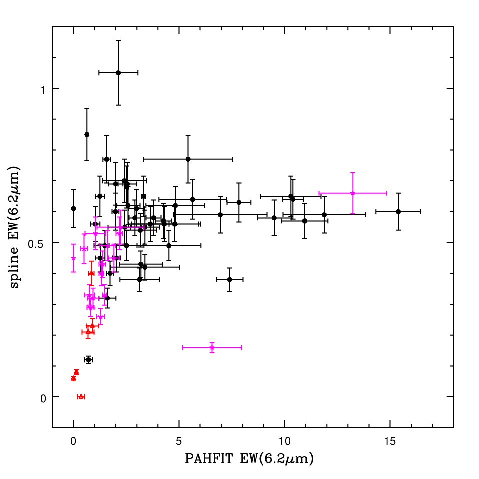
where is the continuum component of Eq. 1. This definition is different from that of S07 in PAHFIT which computes the integral in the range . In the case of the 7.7 micron feature whose FWHM is large and extends the limit of the integral to regions beyond the IRS range where the continuum vanishes arbitrarily, the profile weighted average continuum is used. Despite this caveat, both methods agree within 10% and the discrespancies virtually disappear when increasing the limits of the integral for all other PAHs22 2 In the process of making these comparisons, we discovered two bugs in PAHFIT: 1/ the code was mistakenly calling gaussian profiles instead of Drude profiles to compute the EW integral, thus underestimating EWs by , and 2/ it was applying silicate extinction to the continuum while using the extinction corrected PAH features (according to Eq. 1, both components are equally affected by the extinction term). These bugs are being corrected (J.D. Smith, private communication).. However the EWs measured as above differ significantly from those estimated with the spline method, which consists in fitting a spline function to the continuum from anchor points around the PAH feature, and a Gaussian profile to the continuum-subtracted feature. This method yields considerably smaller EW values as it assigns a non negligible fraction of the PAH flux extracted by PAHFIT to the continuum. Figure 12 shows our EWs (Eq. 3) against the 6.2m PAH EWs computed by [84] for the SSGSS sample assuming a single gaussian on a linear continuum between 5.5m and 6.9m. Their published sample is restricted to SF galaxies defined as having EW(6.2m) m [100]. The measurements for the remaining galaxies were kindly provided by L. Sargsyan. Their formal uncertainty is estimated to be . The two methods are obviously strongly divergent. The spline EWs strongly peak around a value of m with no apparent correlation with the PAHFIT estimates, which reach and can be up to 25 times larger than the [84] values. Our EWs for the main PAH features are listed in Table 3.
The strength of a PAH feature depends on several interwined properties of the ISM: metallicity, radiation field hardness, dust column density, size and ionization state distributions of the dust grains (Dale et al. 2006 and references therein). In particular it is shown to be reduced in extreme far-UV radiation fields, such as AGN-dominated environment [43, 90, 99], near the sites of SF [41, 18, 92, 7, 76, 46] or in very low metallicity environments [35, 101, 74, 68], where the PAH molecules are thought to get destroyed [97, e.g.].


Figure 13 shows the EWs of the main PAH features as a function of [O iii]/H. The Pearson correlation coefficients are indicated at the top right of each panel. AGNs do exhibit noticeably smaller EWs than SF galaxies at short wavelengths (6.2, 7.7 and 8.6m, left panel), however seemingly uncorrelated with radiation field hardness. The range of EWs spanned by AGNs becomes increasingly similar to that of SF galaxies towards longer wavelengths (11.3, 12.7 and 17m, right panel) while at the same time a correlation seems to appear with radiation field hardness. The Pearson coefficients for the AGN population alone at long wavelengths are -0.97, -0.89 and -0.81 respectively from top to bottom, though admittedly they are boosted by the rightmost data point. A larger sample of AGNs is needed to confirm this correlation. PAH strength remains largely independent of radiation field hardness for SF and composite galaxies. These results complement the analysis of [73] who found a correlation between the long-to-short wavelength PAH ratios and [O iii]/H in AGNs. These trends are consistent with the selective destruction of PAH molecules in the hard radiation fields of these sources ([O iii]/H ). The EW trends or lack thereof in Figure 13 suggest that the smallest PAH molecules effective at producing the short-wavelength PAH features get destroyed first, near an AGN, while the larger molecules producing the larger wavelength PAHs require increasingly harder radiation fields for their PAH strength to drop below that of SF galaxies. [33] first suggested that the absence of PAHs could be taken as evidence for the presence of an AGN. Weak PAH emission has since often been used to discriminate between photoionization and accretion disk processes. However the common boundaries for a ‘pure starburt’, e.g. EW(7.7m) [66] or EW(6.2m) m [100] are significantly too weak here, due to the different method we use to compute the equivalent widths as shown above. Based on the PAHFIT decomposition, SF galaxies would be best isolated by EW(6.2m) m, EW(7.7m) m or EW(8.6m)1m, the latter two criteria being more accurately determined in our sample. Those limits are shown as dotted lines in the left panel of Figure 13. The two SF exceptions below the 7.7m and 8.6m EW limits (#32 and #74) happen to have very strong silicate absorption parameters (1.8 and 2.33) and still very distorted absorption-corrected continua compared to the rest of the sample. The dotted lines in the right panel are approximate lower limits for the SF population (EW(11.3m) , EW(12.7m) and EW(17m) ). It is clear that the AGN population becomes increasingly difficult to isolate based on EW alone in the red part of the spectrum.
Figures 14 and 15 show the EWs of the main PAH features as a function Dn(4000) and [N ii]/H respectively. The EWs at short wavelengths show a mild downward trend with increasing age (or decreasing SF activities) while they become independent of it at long wavelengths. This again is consistent with the correlations between the long-to-short wavelength PAH ratios and Dn(4000) or H equivalent width found by [73]. The short wavelength EWs decrease more notably with increasing [N ii]/H ratios, which of course are related to Dn(4000) but appear to be the property that most uniformally and significantly affects the sample as a whole. Metallicity and SF activity are known to affect PAH strength, however, as mentionned earlier, previous studies have demonstrated the opposite effect, namely a decrease in PAH strength at very low metallicity and in intense SF environment. These trends thus make normal blue sequence galaxies the sites of maximum PAH strength.

Other than PAH destruction, another cause of decreasing PAH strength at low wavelengths may be a stronger continuum whose strength may depend on the above parameters. A short wavelength continuum (3–10m) has been observed in AGNs, which is attributed to very hot dust heated by their intense radiation fields (Laurent et al. 2000 and references therein), however the continuum slopes of AGNs in our sample largely overlap those of the SF population (Figure 7). Figure 16 shows the EW of the 7.7m feature as a function of continuum slope, a diagnostic diagram proposed by [61] to distinguish AGNs from PDRs and H ii regions. A clear trend is seen for SF and composite galaxies, suggesting that decreased PAH strength in normal SF galaxies may be at least partly due to an increased continuum at low wavelength, which is itself loosely correlated with Dn(4000) (Figure 7). However the EWs of AGNs appear quite independent of their continuum slope, supporting the PAH destruction scenario. In this diagram, AGNs are expected to populate the lower left side of the plot (shallow slopes and weak PAH features), PDRs the lower right corner (shallow slopes and strong PAH features) and H ii regions the upper left corner of the diagram (steep slopes and weak PAH features). Our SF sequence is qualitatively similar to the location of quiescent SF regions on the Laurent et al. diagram (their Figure 6), which are modeled by a mix of PDR and H ii region spectra, plus an AGN component towards the lower left corner where composite galaxies are indeed most concentrated.


III.3. Diagnostic Diagram
The presence of an AGN is thought to be best verified by the detection of strong high-ionization lines such as [NeV]14.21m or [O iv]25.9m. [43] were the first to show that the ratio of high to low excitation MIR emission lines combined with PAH strength could be used to distinguish AGN activity from star-formation in ULIRGs. This diagnostic was recently revisited by [28] for the nuclear and extra-nuclear regions of normal star-forming galaxies in the SINGS sample observed with the IRS. [28] made use of the [O iv]25.9m/[Ne ii]12.8m emission line ratios with spline derived EWs of the 6.2m feature (they also proposed an alternative diagnostic using the [Si ii]34.8m/[Ne ii]12.8m emission line ratio but [Si ii]34.8m is beyond the usable range of our data). The left panel of Figure 17 shows the Dale et al. diagram using the spline derived EWs of the 6.2m feature measured by [84] in the SSGSS sample. The AGN with no detected [O iv]25.9m line is plotted as an upper limit assuming an [O iv]25.9m/[Ne ii]12.8m line ratio based on the correlation between [Ne ii]12.8m/[O iv]25.9m and [O iii]/H for other AGNs in Figure 10. We applied a cut in error bars to this plot for clarity (log([Ne ii]12.8m/[O iv]25.9m) , roughly the scale of the -axis), which excludes 1 AGN, 1 composite galaxy and 1 SF galaxy. One other AGN is found with no measurable EW. The dotted line represents a variable mix of AGN and SF region; the short solid lines perpendicular to it delineate the AGN region on the left, the SF region at the bottom right, and in between a region of mixed classifications whose physical meaning remains unclear [28]. Given the relative homogeneity of our sample (lacking in extreme types), the very narrow range of spline EWs for ordinary galaxies and the rather large uncertainties in our emission line ratios derived from low resolution spectra, this diagnostic proves of limited use for normal galaxies. Most optically classified SF galaxies do fall into the SF corner, but so do a few composite galaxies. The rest of the sample shows little spread within the mixed region.
Based on the results of this and the previous sections, we revise this diagnostic using the PAHFIT based EWs (Eq. 3) and the correlations between these EWs at low wavelength and [N ii]/H (Figure 15) on the one hand, and between [Ne ii]12.8m/[O iv]25.9m and [O iii]/H (Figure 10) on the other hand. The right panel of Figure 17 shows the [Ne ii]12.8m/[O iv]25.9m emission line ratios against the PAHFIT EWs of the 8.6m feature. Note that we inverted the -axis with respect to the left panel (and the traditional Genzel et al. diagram), so that the figure becomes a flipped version of the optical BPT diagram. The short-dashed lower line is the theoretical optical boundary of [58] translated into this plane using the correlations between EW(8.6m) and [N ii]/H in Figure 15 and between [Ne ii]12.8m/[O iv]25.9m and [O iii]/H in Figure 10 for the AGNs and composite galaxies. Its analytical form is:
| (4) |
where log(EW(8.6m)) and log([Ne ii]12.8m/[O iv]25.9m). The dotted upper line is the empirical boundary of [53] translated using these same correlations for the composite and SF galaxies:
| (5) |
As expected from the poorer correlation between [Ne ii]12.8m/[O iv]25.9m and [O iii]/H for non AGNs, this boundary is less meaningful even though it does isolate the bulk of the SF galaxies. The long-dashed line is an empiral boundary marking the region below which we do not find any SF galaxy:
| (6) |
Despite a mixed region of composite and SF galaxies, there is a clear sequence from the bottom left to the top right of the plots and 3 regions where each optical class is uniquely represented. In particular weak AGNs separate remarkably well in this diagram. The mixed region may in fact be revealing an obscured AGN component in a large fraction () of the optically defined ‘pure’ SF galaxies. Other dust insensitive AGN diagnostics such as X-ray or radio data are necessary to confirm this. Deep XMM observations are available only over a small region of the Lockman Hole and the FIRST radio limits are too bright to reliably test the presence of faint AGNs. Indeed we do not expect this hidden AGN contribution to be large since none of the SF galaxies falls into the AGN corner of the diagram. These objects warrant a detailed study beyond the scope of the present paper.
Alternatively truly ‘pure’ SF galaxies may be defined as lacking the [O iv]25.9m emission line ( of our SF category). These are not represented except for one, which is one of the two SF galaxies with EWs lower than the SF limit in Figs 13, 14 and 15 (EW(8.6m)1m). The lower limit was calculated by arbitrarily assigning it the lowest value of the [OIV] fluxes detected in the sample. The other one, which has a detected [OIV] line, is circled. These 2 galaxies which would have been misclassified as AGNs based on their EW alone sit well into the SF category on this diagram. The AGN with no detected [OIV] (plotted as a lower limit) happens to have the lowest 8.6m EW in the sample. A significantly larger [Ne ii]12.8m/[O iv]25.9m flux ratio would move it into the LINER region of this flipped BPT diagram (although this particular AGN is not optically classified as a LINER). Equations 4, 5 and 6 are reported in Table 4 as well as their equivalents for the 6.2m and 7.7m PAH features. We note that much larger samples, of AGNs in particular, are needed to confirm and/or adjust these relations.
IV. MIR dust components and the total infrared luminosity
In this section we investigate how individual dust components emitting in the narrow MIR region trace the total dust emission in galaxies, which includes a very large FIR component. The definition of the total infrared (TIR) luminosity and the methods used to estimate it varies in the literature [93]. In this paper refers to and has been derived by fitting the Spitzer photometric points (IRAC+IRS Blue Peak Up+MIPS) with [34] model SEDs33 3 http://www.astro.princeton.edu/draine/dust/irem.html and integrating the best fit SED from 3 to 1100m. This is in excellent agreement with the m luminosity derived from the prescription of [26] for MIPS data (their Eq. 4), with a standard deviation of 0.05 dex. This shows that the total IR luminosity really is driven by the MIPS points [25, e.g.]. We note also that integrating the SEDs between 8 and 1000m (sometimes called the FIR luminosity) would decrease the luminosity by dex in the present sample.

Figure 18 shows the correlations between and ratios where equals - from top to bottom - the luminosity of the PAH complexes at 7.7 and 17m, the luminosity of the continuum at 8 and 16m, and the total restframe luminosities in the 8m IRAC band, 16m IRS band and 24m MIPS bands. The continuum and broadband luminosities are defined as . As in all previous figures, SF galaxies are shown as black dots, composite galaxies as pink stars and AGNs as red triangles. The logarithmic scaling factors indicated in each panel are defined as the median of log() for the SF population alone and is represented by the green dashed lines (). The rms and Pearson coefficients of the correlations are also quoted for the SF population alone.
It is striking that galaxies of all types follow the same tight, nearly linear correlations between and the broadband luminosities in all 3 Spitzer bands over 2 dex in luminosity. This implies that all the galaxies in our sample are assigned nearly the same SED from a few m to a thousand m and that the FIR component can be well predicted from any one broadband luminosity in the MIR. This in turn suggests a common heating source for the small and large dust grains responsible for the MIR and FIR emissions respectively [82]. The same correlations apply whether this heating source is stellar or an AGN. Although this may result from the implicit stellar origin of the dust heating in the models, the source of ionizing radiation may not significantly affect the broad SED, at least for weak AGNs. Many attempts have been made to derive calibrations between and single MIR broadband luminosities [21, 37, 93, 83, 11, 6, 104]. Our best fit slope at 16m ( ) is in good agreement with that of [21] for the 15m ISO fluxes. At 24m our correlation for SF galaxies ( ) is more linear than found in other studies [93, 83, 104, 6] but the discrepancy with the first three calibrations [93, 83, 104] disappears when including composite galaxies into the fit ( ). On the other hand our correlation is in excellent agreement with the [71] sample (hereafter MK06).

The PAH and continuum luminosities also correlate remarkably tightly and nearly linearly with , however with some distinctions between AGNs and SF galaxies and between the hot and cool parts of the spectrum. The scatter between and PAH luminosity for SF galaxies is larger for the 17m PAH feature than for the 7.7m PAH feature. AGNs and composite galaxies blend with the SF population in the 17m feature correlation whereas they tend to have lower PAH luminosities at 7.7m and stronger 8m continua for the same . The residuals are shown in Figure 19 as a function of the corresponding equivalent widths. The relations between these residuals and EWs are of course expected since the total flux at 8 and 16m can be nearly perfectly substituted for for SF galaxies and AGNs alike in the left and right panels respectively (the dotted lines show the predicted relations assuming these substitutions). The most scattered correlation is found with the continuum luminosity at 8m. This may be due to larger measurement errors since this continuum is faint and/or a stellar contribution unrelated to . A more speculative reason may be that this continuum originates from high intensity radiation fields only and is thus uncorrelated with the cold component of , unlike the PAH emission.
The scaling factors are listed in Table 5 for the main PAH features and the Spitzer band luminosities. We also add to our list of MIR components the peak luminosity of the 7.7m PAH feature, defined as , as it is a more easily measurable quantity at high redshift than the integrated flux of the PAH feature [100, 84]. For galaxies with EWm (most SF galaxies), the median ratio of this peak luminosity to the total luminosity of the PAH complex, , is and the peak luminosity estimates the total PAH luminosity to within 20%. However the overestimate can be as large as 50% for other galaxy types in this sample, in particular galaxies containing an AGN which may not be easily isolated in high redshift samples and may also have much smaller EWs leading to yet larger errors.
For the calibration that shows the strongest deviation from linearity in Figure 18, which is found for the 7.7m PAH luminosity (), the linear approximation (where ) recovers within a factor of 1.5 in this sample. For starbursts and ULIRG starbursts, [80] found a mean log of 2.09 and 2.26 respectively, considerably larger than for normal galaxies. More recently [67] find a mean logarythmic ratio of 1.52 for a sample of starburst nuclei, closer to our value. Our mean logarythmic ratio for the 6.2m feature is 1.5 and 2.0 with and without aperture correction respectively while [88] find a value of 2.4 for a sample of normal and starburst nuclei. This ratio is yet higher (3.2) in Galactic H ii regions while highly embedded star-forming regions can lack PAH emission altogether [75]. These increased ratios for starburst regions compared to normal SF galaxies are generally attributed to PAH destruction near the site of on-going SF due to intense radiation fields, making PAHs poor tracers of SF (Peeters et al. 2004 and references therein). The EW dependence of the log ratio is clearly seen within our sample in the upper left panel of Figure 19. This cautions against the use of a single linear relation between PAH luminosity and for galaxies of unknown physical properties.
However independently of galaxy type we expect to find lower values than these studies which all made use of interpolation methods to extract the PAH features. Using a Lorentzian profile fitting method comparable to PAHFIT for a sample of starburst-dominated LIRGS at , [48] find mean log ratios of , and for the 6.2, 7.7 and 11.3m features respectively. These ratios are 2.6, 1.8, and 1.4 times larger than ours respectively, closer than previous studies despite the quite different galaxy type considered. The wavelength gradient can be explained in the context of selective PAH destruction.
Finally we note that in our sample the total m PAH luminosity amounts to of the total IR luminosity for SF galaxies, for composite galaxies and for AGNs. The 7.7m feature alone accounts for of the total PAH emission. These fractional contributions are in good agreement with those found in the SINGS sample (S07).

V. MIR components and the Star-Formation Rate
The TIR luminosity is a robust tracer of the SFR for very dusty starbursts, whose stellar emission is dominated by young massive stars and almost entirely absorbed by dust (typically galaxies with depleted PAH emission), but for more quiescent and/or less dusty galaxies such as those in the present sample, it can include a non negligible contribution from dust heated by evolved stars (‘cirrus emission’) as well as miss a non negligible fraction of the young stars’ emission that is not absorbed by dust [65]. For normal spiral galaxies the contribution of non ionizing photons may actually dominate the dust heating over H ii regions [36, 35] while low dust opacity makes these galaxies H and UV bright. The tight correlations between MIR luminosities and indicate that the same caveats apply from the MIR to the FIR [9].
V.1. MIR dust and H
H emission is a more direct quantifier of young massive stars - in the absence of AGN - but inversely it must be corrected for the fraction that gets absorbed by dust. The SDSS line fluxes are corrected for foreground (galactic) reddening using [72]. The correction for intrinsic extinction is usually done using the Balmer decrement and an extinction curve to first order, or more accurately with higher order hydrogen lines [12]. Here we correct the SDSS H fluxes in the usual simple way using the stellar-absorption corrected H/H ratio and a Galactic extinction curve. We assumed an intrinsic H/H ratio of 2.86 (case B recombination at electron temperature and density ) and (the mean value for the diffuse ISM). The H attenuations range from 0.4 to 2.3 mag in the SF galaxy subsample with a median value of 1.1 mag, meaning that between 10 and 70% of the H photons do not get reemitted in the IR.
The SDSS H measurements also require fiber aperture corrections. Here again we apply the usual method which consists in scaling the fiber-measured H fluxes using the -band Petrosian-to-fiber flux ratios [51]. The mean value for these ratios is 3.5. The left panels of Figure 20 shows the extinction and aperture corrected H luminosity, , against the TIR and 24m continuum luminosities (top and bottom panel respectively). The rms and slope of the linear regressions (solid lines) are indicated for the SF population alone. The logarithmic scaling factors indicated in each panel are defined as the median of log() also for the SF population alone. The green dashed lines indicate equality (). Overlaid are the MK06 data (open green squares) and SINGS data (open blue squares for the integrated measurements, crosses for 20”x20” galaxy center measurements), taken from [54] (hereafter K09).
Our median to logarithmic ratio of is in good agreement with the ratio of SFR calibration coefficients derived by [55] for H and respectively, implying that (and the MIR components that correlate with it) may be reasonable SFR tracers in normal SF galaxies after all. This may actually be a coincidence due to the fact that the cirrus emission and the unattenuated ionizing flux roughly cancel each other in massive spiral galaxies (K09 and references therein). Our ratio is also in good agreement with the MK06 sample (). In recent years several groups have exploited the capabilities of Spitzer to re-investigate the relationship between MIR components and H emission. Our mean to logarithmic ratio of is in good agreememt with these [101, 104, 54, e.g.], as is the higher mean ratio for composite galaxies [104]. However the slope of our correlations for SF galaxies tend to be more linear than found in these studies (the dotted lines in Figure 20 show fits to the MK06 sample). Yet non linearity is expected from the positive correlation between attenuation and SFR. Given the good agreement between our and the MK06 samples in the IR (cf. the – correlation in the previous section), differences in H measurements must be responsible for the discrepancy in slopes. In particular it is possible that aperture corrections, which are not needed for the MK06 sample, are overestimated for all or a fraction of our galaxies. This would be the case if SF is more intense at the center of the galaxies and/or more attenuated, a common occurence in spiral galaxies [15, e.g.].
As a test we consider the smaller aperture corrections derived by [12] (hereafter B04) that rely on the likelihood distribution of the specific SFR as a function of colors. These corrections depend on the galaxy colors outside the fiber which are not necessarily the same as inside, and are on average smaller than the -band corrections for SF galaxies. The right panels of Figure 20 shows the same relations as in the left panels using these smaller aperture corrections. The new correlations (solid lines) are indeed steeper while the higher mean and logarithmic ratios of and respectively remain within the range of the MK06 sample.

More dramatic is the effect on the relation between H attenuation and the ratio of , or other IR luminosity, to , the ‘observed’ (aperture-corrected but attenuation-uncorrected) H luminosity. This relation is shown in Figure 21 for both types of aperture correction. K09 modelled the H attenuation as:
| (7) |
equivalent to . This energy balance approach was introduced by [14], [77] and [57] to correct H fluxes but has long been used to estimate UV attenuations from the ratios [70, e.g.]. The solid lines in both panels of Figure 21 show the best fits by K09 for the SINGS and MK06 samples (). The dashed lines are best fits for the SSGSS sample ( in the top panel and in the bottom panel). The smaller aperture corrections used in the bottom panel significantly improves the fit and the agreement between the three samples. Unless otherwise stated we now assume these corrections in the rest of the paper.

Figure 22 shows the to ratios as a function of for the TIR, 24m continuum, 7.7m and 17m PAH luminosities. The coefficients are indicated at the top left of each panel for the SF population. The rms and Pearson coefficients are also indicated for the SF population. For the TIR and 24m luminosities, and are best fits to Eq. 7 for the SINGS+MK06 samples by K09. The combinations of and or provide a very tight (rms=0.08) and perfectly linear fit to the total H luminosity for all samples combined over 5 dex in luminosity, as was shown by K09 for the SINGS and MK06 samples. Composite galaxies follow nearly the same relation save for 2 over-corrected outliers. Although more scattered AGNs also follow the SF population. For the PAH luminosities, and are best fits to Eq. 7 for the present sample. Here also the combinations of and PAH luminosities provide a much improved fit to the total H luminosity compared to the raw relations (not shown), including for composite galaxies and AGNs with the exception of a few outliers, most notably a composite galaxy with no H attenuation and a large IR/H ratio (#84).
The same exercise can be performed with similarly good results with any other MIR dust components. The and coefficients for the SSGSS sample are listed in Table 5. Note that , using the scaling factors listed in the first column of Table 5. Although the factors and depend on the specific definition of and on the models used to compute it, the coefficients for specific dust components or MIR broadband luminosities, which are easier to measure than the total IR, are independent of these choices.
As stated above the smaller B04 corrections seem to be more appropriate than the usual -band corrections given the agreement with data that do not require aperture corrections. However they are not trivially calculated (see B04 for details of the modeling). More importantly H is often not easily measurable at all. It is therefore useful to provide SFR recipes based on a single IR quantity, or on a combination of IR and UV measurements (see next section) as UV is more easily obtained at high redshifts. Table 5 lists the mean ratios of the SF population for the various MIR components. Keeping in mind the non linearities and scatter in the true relations, SFRs can be estimated from these approximate H luminosities using K09’s calibration (derived from the latest Starburst99 models and assuming a Kroupa IMF and solar metallicity):
| (8) |
As an example, the SFR derived from the MIPS 24m luminosity would be SFR consistent with Rieke et al. (2009) for galaxies in the range of TIR luminosities of the present sample.

As Eq. 8 was shown by B04 to underestimate the SFR of massive galaxies and thus may not be appropriate for this sample or at high , we also add to Table 5 calibrations where is the SFR derived by these authors as follows: they computed SFR likelihood distributions of SF galaxies in the SDSS spectroscopic sample by fitting all strong emission lines simultaneously using the [20] models and assuming a Kroupa IMF. Dust was accounted for using the [19] multicomponent model which provides a consistent treatment of the attenuation of both continuum and emission line photons. refers to the medians of these SFR distributions. In this model, the H attenuation increases with mass while the ratio of to SFR decreases with mass so that the same observed H luminosity signals a noticeably higher SFR in higher mass galaxies than predicted from Kennicutt’s relation. We refer to B04 for full details. is found to be in good agreement with Eq. 8 for average local galaxies but diverges from it for higher mass, higher metallicity galaxies such as found in the present sample where is on average twice larger within the SDSS fiber than derived from the Kennicutt relation. However the aperture corrections in this study being smaller than derived from the -band magnitudes for SF galaxies, the total are only times larger than derived conventionally using the Balmer decrements, -band aperture corrrections and Eq. 8. For composite galaxies and AGNs, is not estimated from the emission lines which are contaminated by AGN emission, but in a statistical way based on the correlation between Dn(4000) and the specific SFR. We exclude those for clarity.
Figure 23 shows the relations between and the ratios for the TIR, 24m continuum, 7.7m and 17m PAH luminosities. As in previous figures the correlation parameters are quoted at the bottom right of each panel. These correlations are more scattered and less linear (higher rms and Pearson coefficient) than with . The attenuations underlying being larger than those derived from the Balmer decrement for massive galaxies, the to ratio: is very close to that of Kennicutt et al. (1998) for opaque starburst galaxies (taking into account the difference in IMFs). The calibrations are listed in Table 5.
V.2. MIR dust and UV
Turning now to UV data where dust attenuation is an inevitable issue, we once again follow an energy balance approach [70, 45, 59, 13, 23, 104, 54]. SFRs can be estimated from dust corrected FUV luminosities using the following calibration by K09 assuming a Kroupa IMF, solar metallicity, and adjusted to the GALEX FUV filter (Å).
| (9) |
where is the dust-corrected GALEX FUV luminosity.


Assuming equality with a known SFR estimate (e.g. or ), we derive FUV attenuations as follows:
| (10) |
where is the observed FUV luminosity in . Figure 24 shows the FUV attenuations of the SF subsample derived from Eq. 10 as a function of (known as the infrared excess or IRX) assuming assuming SFR= (Eq. 8, top panel) and (bottom panel). The median FUV attenuations are 1.9 and 2.8 magnitudes respectively, corresponding to 83 and 92% of the FUV light being absorbed by dust (note that assuming conventional -band aperture corrections for H yields exactly intermediate values). The dotted line is a theoretical relation by [13]; the dashed lines shows a model derived by [23] for galaxies with corresponding to the mean color of our sample (these authors modeled the dependence of the IRX/ relation with the age of the underlying stellar populations, or specific SFR, or color). The solid lines are best fits of the form:
| (11) |
equivalent to , i.e. , following K09’s method. Our best fit parameters are and 0.729 in the top and bottom panels respectively. However all three models are poor in the bottom panel. FUV attenuations assuming are best modeled by a linear function of log(IRX) or FUV-optical colors [95]. Assuming (top panel) the FUV attenuations are well fit both by [23] and by Eq. 11. In this case a linear combination of and or recovers with low scatter as shown in Figure 25 using the TIR, 24m continuum, 7.7m and 17m luminosities. As with H in the previous section, similarly good corrections can be achieved using other MIR components. The and coefficients are listed in Table 5.
V.3. Neon emission lines

As put forward by [49], [Ne ii]12.8m is an excellent tracer of ionizing stars, being an abundant and dominant species in H ii regions, quite insensitive to density, as well as to dust given its long wavelength. [Ne iii]15.5m has similar properties but can be the dominant species in e.g. low-mass, low-metallicity galaxies [74, 102]. Thus Ne emission is expected to be directly comparable to the dust corrected H emission. Using the CLOUDY code [39], we find that the ionizing flux from stars hotter than 10K is best represented by the following weighted linear combination of [Ne ii]12.8m and [Ne iii]15.5m also including a metallicity dependence:
| (12) |
where is the metallicity in solar units. We use the right hand side of this equation to define the neon flux and luminosity, .
For the sake of comparison with the study of [49] who used as SFR estimate, as well as a straight sum of [Ne ii]12.8m and [Ne iii]15.5m, we note that our ([Ne ii]12.8m+[Ne iii]15.5m) to ratio is consistent with the IRS dataset used by these authors [74, 102]. Our ([Ne ii]12.8m) to ratio is larger but this may be explained by the large number of low metallicity galaxies in the samples used, in particular the [102] dataset which specifically targets low-metallicity blue compact dwarf galaxies for which [Ne iii]15.5m is the dominant Ne species (cf. Figure 11).
The left panels of Figure 26 shows the / and / ratios as a function of (a) and (b) respectively. Only SF galaxies with measured metallicity are represented (85%). Surprisingly behaves much like the MIR dust components. It traces fairly linearly and tightly the total IR luminosity while we can define using Eq. 7 such that provides the tightest and most linear correlation with , as shown in the lower right panel (d) of Figure 26. Likewise we can define such that provides a good fit to . The upper right panel (c) shows the to ratio against , which is significantly more scattered than the previous relations as with the MIR dust components. This correlation implies the following calibration:
| (13) |
The and coefficient as well as the median /, / and / ratios are reported in Table 5.
V.4. Molecular Hydrogen lines

The rotational H2 lines are fainter than the [NeII]12.9m, [Ne iii]15.5m and [S iii]18.7m lines for most galaxies in our sample but molecular hydrogen represents a significant mass fraction of the ISM in normal galaxies. The main excitation source of the rotational transitions is expected to be FUV radiation from massive stars in PDRs [50, and references therein], therefore these lines also trace SF. The first study of warm molecular hydrogen ( K) in the nuclei of normal, low luminosity galaxies was presented by [81] (hereafter R07) using the SINGS sample. A major result of their work is the tight correlation between the sum of the to rotational lines (noted ) and the PAH emission, with a /PAH ratio insensitive to the intensity of the radiation field. This correlation is interpreted as supporting the origin of H2 excitation within PDRs (defined by [50] as including the neutral ISM illuminated by FUV photons), with fluorescence as the dominant excitation mechanism.
Our median logarithmic ratios of to the TIR, 24m MIPS band and 7.7m PAH luminosities for the SF population are , and respectively. The first two ratios are 1.6 and 1.8 times larger respectively than those of R07 for H ii nuclei (taking into account that R07 assumed a filter width of 3.1THz instead of for the 24m band). On the other hand our /PAH ratio using the stellar component subtracted 8m IRAC flux instead of the PAHFIT extracted feature following R07, is only 1.2 times higher than that of R07. These differences are within uncertainties but the gradients may also reflect real differences between H ii nuclei and disks (warm H2 more abundant in disks), as well as support the physical link between warm H2 and PAH emissions suggested by R07.
Unlike R07 we do not find significantly higher or ratios for AGNs (see also the top panel of Figure 10). This may also be due to the much lower AGN contribution when disks are included. R07 interpret the higher AGN ratios as an excess of H2 emission, attributed to additional mechanisms exciting H2 molecules in AGNs. The ratio does show a significant excess for AGNs, however this excess correlates with PAH EWs, suggesting that depleted PAHs in AGNs contribute in part to the effect. Our dispersion for the ratio is also comparable to the other two while R07 find it to be significantly tighter in H ii nuclei, especially than the ratio. Our results suggest that local complexities are largely washed out on galactic scale and that warm molecular hydrogen traces dust in all its forms when considering integrated measurements.
The left panels of Figure 27 show the to and ratios as a function of (a) and (b). Like , traces reasonably linearly and tightly the total IR luminosity while the correlation with is improved with a linear combination of and using Eq. 7 () (c). Likewise the upper right panel (d) shows the to ratio against , which implies the following calibration:
| (14) |
All the coefficients are reported in Table 5.
VI. Summary and Conclusions
We present a MIR spectroscopic survey of 100 ‘normal’ galaxies at with the goal of investigating the use of mid-infrared PAH features, continuum and emission lines as probes of their star-formation and AGN activity. Available data include GALEX UV photometry, SDSS optical photometry and spectroscopy, and Spitzer near to far-infrared photometry. The optical spectroscopic data in particular allow us to classify these galaxies into star-forming, composite and AGNs, according to the standard optical “BPT” diagnotic diagram. The MIR spectra were obtained with the low resolution modules of the Spitzer IRS and decomposed into unattenuated features and continuum using the PAHFIT code of [86]. A notable feature of this decomposition method is to extract a much larger PAH contribution (and proportionally smaller continuum contribution) from the total flux compared to standard spline fitting methods which anchor the continuum in the wings of the features where non negligible PAH power remain. As a consequence, the PAH equivalenth widths are not only larger but extend over a considerably larger dynamic range (e.g. the equivalent widths of the 6.2 and 7.7m PAH features in our sample extend to 15 and 32m respectively).
We study the variations of the various MIR spectral components as a function of the optically derived age (as measured by the 4000Å break index), radiation field hardness (as measured by the [O iii]/H ratio) and metallicity (as measured by [N ii]/H ratio) of the galaxies. Systematic trends are found despite the lack of extreme objects in the sample, in particular between PAH strength at low wavelength and gas phase metallicity, and between the ratio of high to low excitation lines (e.g. [O iv]25.9m/[Ne ii]12.8m) and radiation field hardness. These trends confirm earlier results detected in sources with higher surface brightnesses such as ULIRGS, strong AGNs and H ii nuclei. Our results are consistent with the selective destruction in AGN radiation fields of the smallest PAH molecules efficient at producing the low wavelength PAH features (6.2 to 8.6m). They also suggest that radiation fields harder than those in the present sample would also destroy larger PAH molecules responsible for the longer wavelength features (11.3 to 17m). Aging galaxies also tend to show weaker low wavelength PAH features, consistent with their main origin in star-forming regions.
We revisit the MIR diagnostic diagram of Genzel et al. (1998) relating PAH equivalent widths and [Ne ii]12.8m/[O iv]25.9m emission line ratios. Based on the strongest trends we observed between these measurements and optical emission line ratios and thanks to the extended range of equivalent widths provided by PAHFIT, we find this diagnostic to closely resemble the optical “BPT” diagram, with a much improved resolving power for normal galaxies than previously found based on spline derived equivalent widths. A mixed region of star-forming and composite galaxies remains, which may be revealing obscured AGNs in a large fraction of the optically defined ‘pure’ star-forming galaxies.
We find tight and nearly linear correlations between the total infrared luminosity of star-forming galaxies and the luminosity of individual MIR components, including PAH features, continuum, neon emission lines and molecular hydrogen lines. This implies that these individual MIR components are good gauges of the total dust emission on galactic scale despite different spatial and physical origins on the scale of star-forming regions. Following the approach of [54] based on energy balance arguments, we show that like the total infrared luminosity, these individual components can be used to estimate dust attenuation in the UV and in the H lines. Given the non negligible attenuation in these IR selected galaxies, the correlations between the MIR and dust corrected H luminosities can also provide first order estimates of the SFR. We thus propose average scaling relations between the various MIR components and H derived star-formation rates.
References
- [1] Allamandola, L. J., Tielens, A. G. G. M., & Barker, J. R. 1985, ApJ, 290, L25
- [2] Alonso-Herrero, A., Pereira-Santaella, M., Rieke, G. H., Colina, L., Engelbracht, C. W., Perez-Gonzalez, P., Diaz-Santos, T., & Smith, J. D. T. 2009, ArXiv e-prints
- [3] Armus, L., Charmandaris, V., Bernard-Salas, J., Spoon, H. W. W., Marshall, J. A., Higdon, S. J. U., Desai, V., Teplitz, H. I., Hao, L., Devost, D., Brandl, B. R., Wu, Y., Sloan, G. C., Soifer, B. T., Houck, J. R., & Herter, T. L. 2007, ApJ, 656, 148
- [4] Baldwin, J. A., Phillips, M. M., & Terlevich, R. 1981, PASP, 93, 5
- [5] Balogh, M. L., Schade, D., Morris, S. L., Yee, H. K. C., Carlberg, R. G., & Ellingson, E. 1998, ApJ, 504, L75+
- [6] Bavouzet, N., Dole, H., Le Floc’h, E., Caputi, K. I., Lagache, G., & Kochanek, C. S. 2008, A&A, 479, 83
- [7] Beirão, P., Brandl, B. R., Devost, D., Smith, J. D., Hao, L., & Houck, J. R. 2006, ApJ, 643, L1
- [8] Bendo, G. J., Draine, B. T., Engelbracht, C. W., Helou, G., Thornley, M. D., Bot, C., Buckalew, B. A., Calzetti, D., Dale, D. A., Hollenbach, D. J., Li, A., & Moustakas, J. 2008, MNRAS, 389, 629
- [9] Boselli, A., Lequeux, J., & Gavazzi, G. 2004, A&A, 428, 409
- [10] Boulanger, F., Beichman, C., Désert, F. X., Helou, G., Perault, M., & Ryter, C. 1988, ApJ, 332, 328
- [11] Brandl, B. R., Bernard-Salas, J., Spoon, H. W. W., Devost, D., Sloan, G. C., Guilles, S., Wu, Y., Houck, J. R., Weedman, D. W., Armus, L., Appleton, P. N., Soifer, B. T., Charmandaris, V., Hao, L., Higdon, J. A. M. S. J., & Herter, T. L. 2006, ApJ, 653, 1129
- [12] Brinchmann, J., Charlot, S., White, S. D. M., Tremonti, C., Kauffmann, G., Heckman, T., & Brinkmann, J. 2004, MNRAS, 351, 1151
- [13] Buat, V., Iglesias-Páramo, J., Seibert, M., Burgarella, D., Charlot, S., Martin, D. C., Xu, C. K., Heckman, T. M., Boissier, S., Boselli, A., Barlow, T., Bianchi, L., Byun, Y.-I., Donas, J., Forster, K., Friedman, P. G., Jelinski, P., Lee, Y.-W., Madore, B. F., Malina, R., Milliard, B., Morissey, P., Neff, S., Rich, M., Schiminovitch, D., Siegmund, O., Small, T., Szalay, A. S., Welsh, B., & Wyder, T. K. 2005, ApJ, 619, L51
- [14] Calzetti, D., Kennicutt, R. C., Engelbracht, C. W., Leitherer, C., Draine, B. T., Kewley, L., Moustakas, J., Sosey, M., Dale, D. A., Gordon, K. D., Helou, G. X., Hollenbach, D. J., Armus, L., Bendo, G., Bot, C., Buckalew, B., Jarrett, T., Li, A., Meyer, M., Murphy, E. J., Prescott, M., Regan, M. W., Rieke, G. H., Roussel, H., Sheth, K., Smith, J. D. T., Thornley, M. D., & Walter, F. 2007, ApJ, 666, 870
- [15] Calzetti, D., Kennicutt, Jr., R. C., Bianchi, L., Thilker, D. A., Dale, D. A., Engelbracht, C. W., Leitherer, C., Meyer, M. J., Sosey, M. L., Mutchler, M., Regan, M. W., Thornley, M. D., Armus, L., Bendo, G. J., Boissier, S., Boselli, A., Draine, B. T., Gordon, K. D., Helou, G., Hollenbach, D. J., Kewley, L., Madore, B. F., Martin, D. C., Murphy, E. J., Rieke, G. H., Rieke, M. J., Roussel, H., Sheth, K., Smith, J. D., Walter, F., White, B. A., Yi, S., Scoville, N. Z., Polletta, M., & Lindler, D. 2005, ApJ, 633, 871
- [16] Cao, C., Xia, X. Y., Wu, H., Mao, S., Hao, C. N., & Deng, Z. G. 2008, MNRAS, 390, 336
- [17] Cesarsky, C. J. & Sauvage, M. 1999, Ap&SS, 269, 303
- [18] Cesarsky, D., Lequeux, J., Abergel, A., Perault, M., Palazzi, E., Madden, S., & Tran, D. 1996, A&A, 315, L309
- [19] Charlot, S. & Fall, S. M. 2000, ApJ, 539, 718
- [20] Charlot, S. & Longhetti, M. 2001, MNRAS, 323, 887
- [21] Chary, R. & Elbaz, D. 2001, ApJ, 556, 562
- [22] Compiègne, M., Abergel, A., Verstraete, L., Reach, W. T., Habart, E., Smith, J. D., Boulanger, F., & Joblin, C. 2007, A&A, 471, 205
- [23] Cortese, L., Boselli, A., Franzetti, P., Decarli, R., Gavazzi, G., Boissier, S., & Buat, V. 2008, MNRAS, 386, 1157
- [24] da Cunha, E., Charlot, S., & Elbaz, D. 2008, MNRAS, 388, 1595
- [25] Dale, D. A., Gil de Paz, A., Gordon, K. D., Hanson, H. M., Armus, L., Bendo, G. J., Bianchi, L., Block, M., Boissier, S., Boselli, A., Buckalew, B. A., Buat, V., Burgarella, D., Calzetti, D., Cannon, J. M., Engelbracht, C. W., Helou, G., Hollenbach, D. J., Jarrett, T. H., Kennicutt, R. C., Leitherer, C., Li, A., Madore, B. F., Martin, D. C., Meyer, M. J., Murphy, E. J., Regan, M. W., Roussel, H., Smith, J. D. T., Sosey, M. L., Thilker, D. A., & Walter, F. 2007, ApJ, 655, 863
- [26] Dale, D. A. & Helou, G. 2002, ApJ, 576, 159
- [27] Dale, D. A., Helou, G., Contursi, A., Silbermann, N. A., & Kolhatkar, S. 2001, ApJ, 549, 215
- [28] Dale, D. A., Smith, J. D. T., Armus, L., Buckalew, B. A., Helou, G., Kennicutt, Jr., R. C., Moustakas, J., Roussel, H., Sheth, K., Bendo, G. J., Calzetti, D., Draine, B. T., Engelbracht, C. W., Gordon, K. D., Hollenbach, D. J., Jarrett, T. H., Kewley, L. J., Leitherer, C., Li, A., Malhotra, S., Murphy, E. J., & Walter, F. 2006, ApJ, 646, 161
- [29] Dale, D. A., Smith, J. D. T., Schlawin, E. A., Armus, L., Buckalew, B. A., Cohen, S. A., Helou, G., Jarrett, T. H., Johnson, L. C., Moustakas, J., Murphy, E. J., Roussel, H., Sheth, K., Staudaher, S., Bot, C., Calzetti, D., Engelbracht, C. W., Gordon, K. D., Hollenbach, D. J., Kennicutt, R. C., & Malhotra, S. 2009, ApJ, 693, 1821
- [30] Deo, R. P., Richards, G. T., Crenshaw, D. M., & Kraemer, S. B. 2009, ApJ, 705, 14
- [31] Desai, V., Armus, L., Spoon, H. W. W., Charmandaris, V., Bernard-Salas, J., Brandl, B. R., Farrah, D., Soifer, B. T., Teplitz, H. I., Ogle, P. M., Devost, D., Higdon, S. J. U., Marshall, J. A., & Houck, J. R. 2007, ApJ, 669, 810
- [32] Désert, F., Boulanger, F., & Puget, J. L. 1990, A&A, 237, 215
- [33] Désert, F. X. & Dennefeld, M. 1988, A&A, 206, 227
- [34] Draine, B. T. & Li, A. 2007, ApJ, 657, 810
- [35] Dwek, E. 2005, in American Institute of Physics Conference Series, Vol. 761, The Spectral Energy Distributions of Gas-Rich Galaxies: Confronting Models with Data, ed. C. C. Popescu & R. J. Tuffs, 103–122
- [36] Dwek, E., Fioc, M., & Varosi, F. 2000, in Lecture Notes in Physics, Berlin Springer Verlag, Vol. 548, ISO Survey of a Dusty Universe, ed. D. Lemke, M. Stickel, & K. Wilke, 157–+
- [37] Elbaz, D., Cesarsky, C. J., Chanial, P., Aussel, H., Franceschini, A., Fadda, D., & Chary, R. R. 2002, A&A, 384, 848
- [38] Farrah, D., Bernard-Salas, J., Spoon, H. W. W., Soifer, B. T., Armus, L., Brandl, B., Charmandaris, V., Desai, V., Higdon, S., Devost, D., & Houck, J. 2007, ApJ, 667, 149
- [39] Ferland, G. J., Korista, K. T., Verner, D. A., Ferguson, J. W., Kingdon, J. B., & Verner, E. M. 1998, PASP, 110, 761
- [40] Förster Schreiber, N. M., Roussel, H., Sauvage, M., & Charmandaris, V. 2004, A&A, 419, 501
- [41] Geballe, T. R., Tielens, A. G. G. M., Allamandola, L. J., Moorhouse, A., & Brand, P. W. J. L. 1989, ApJ, 341, 278
- [42] Genzel, R. & Cesarsky, C. J. 2000, ARA&A, 38, 761
- [43] Genzel, R., Lutz, D., Sturm, E., Egami, E., Kunze, D., Moorwood, A. F. M., Rigopoulou, D., Spoon, H. W. W., Sternberg, A., Tacconi-Garman, L. E., Tacconi, L., & Thatte, N. 1998, ApJ, 498, 579
- [44] Giard, M., Bernard, J. P., Lacombe, F., Normand, P., & Rouan, D. 1994, A&A, 291, 239
- [45] Gordon, K. D., Clayton, G. C., Witt, A. N., & Misselt, K. A. 2000, ApJ, 533, 236
- [46] Gordon, K. D., Engelbracht, C. W., Rieke, G. H., Misselt, K. A., Smith, J., & Kennicutt, Jr., R. C. 2008, ApJ, 682, 336
- [47] Helou, G., Roussel, H., Appleton, P., Frayer, D., Stolovy, S., Storrie-Lombardi, L., Hurt, R., Lowrance, P., Makovoz, D., Masci, F., Surace, J., Gordon, K. D., Alonso-Herrero, A., Engelbracht, C. W., Misselt, K., Rieke, G., Rieke, M., Willner, S. P., Pahre, M., Ashby, M. L. N., Fazio, G. G., & Smith, H. A. 2004, ApJS, 154, 253
- [48] Hernán-Caballero, A., Pérez-Fournon, I., Hatziminaoglou, E., Afonso-Luis, A., Rowan-Robinson, M., Rigopoulou, D., Farrah, D., Lonsdale, C. J., Babbedge, T., Clements, D., Serjeant, S., Pozzi, F., Vaccari, M., Montenegro-Montes, F. M., Valtchanov, I., González-Solares, E., Oliver, S., Shupe, D., Gruppioni, C., Vila-Vilaró, B., Lari, C., & La Franca, F. 2009, MNRAS, 395, 1695
- [49] Ho, L. C. & Keto, E. 2007, ApJ, 658, 314
- [50] Hollenbach, D. J. & Tielens, A. G. G. M. 1997, ARA&A, 35, 179
- [51] Hopkins, A. M., Miller, C. J., Nichol, R. C., Connolly, A. J., Bernardi, M., Gómez, P. L., Goto, T., Tremonti, C. A., Brinkmann, J., Ivezić, Ž., & Lamb, D. Q. 2003, ApJ, 599, 971
- [52] Houck, J. R., Roellig, T. L., van Cleve, J., Forrest, W. J., Herter, T., Lawrence, C. R., Matthews, K., Reitsema, H. J., Soifer, B. T., Watson, D. M., Weedman, D., Huisjen, M., Troeltzsch, J., Barry, D. J., Bernard-Salas, J., Blacken, C. E., Brandl, B. R., Charmandaris, V., Devost, D., Gull, G. E., Hall, P., Henderson, C. P., Higdon, S. J. U., Pirger, B. E., Schoenwald, J., Sloan, G. C., Uchida, K. I., Appleton, P. N., Armus, L., Burgdorf, M. J., Fajardo-Acosta, S. B., Grillmair, C. J., Ingalls, J. G., Morris, P. W., & Teplitz, H. I. 2004, ApJS, 154, 18
- [53] Kauffmann, G., Heckman, T. M., Tremonti, C., Brinchmann, J., Charlot, S., White, S. D. M., Ridgway, S. E., Brinkmann, J., Fukugita, M., Hall, P. B., Ivezić, Ž., Richards, G. T., & Schneider, D. P. 2003, MNRAS, 346, 1055
- [54] Kennicutt, R. C., Hao, C., Calzetti, D., Moustakas, J., Dale, D. A., Bendo, G., Engelbracht, C. W., Johnson, B. D., & Lee, J. C. 2009, ApJ, 703, 1672
- [55] Kennicutt, Jr., R. C. 1998, ApJ, 498, 541
- [56] Kennicutt, Jr., R. C., Armus, L., Bendo, G., Calzetti, D., Dale, D. A., Draine, B. T., Engelbracht, C. W., Gordon, K. D., Grauer, A. D., Helou, G., Hollenbach, D. J., Jarrett, T. H., Kewley, L. J., Leitherer, C., Li, A., Malhotra, S., Regan, M. W., Rieke, G. H., Rieke, M. J., Roussel, H., Smith, J., Thornley, M. D., & Walter, F. 2003, PASP, 115, 928
- [57] Kennicutt, Jr., R. C., Calzetti, D., Walter, F., Helou, G., Hollenbach, D. J., Armus, L., Bendo, G., Dale, D. A., Draine, B. T., Engelbracht, C. W., Gordon, K. D., Prescott, M. K. M., Regan, M. W., Thornley, M. D., Bot, C., Brinks, E., de Blok, E., de Mello, D., Meyer, M., Moustakas, J., Murphy, E. J., Sheth, K., & Smith, J. D. T. 2007, ApJ, 671, 333
- [58] Kewley, L. J., Dopita, M. A., Sutherland, R. S., Heisler, C. A., & Trevena, J. 2001, ApJ, 556, 121
- [59] Kong, X., Charlot, S., Brinchmann, J., & Fall, S. M. 2004, MNRAS, 349, 769
- [60] Kroupa, P. 2001, MNRAS, 322, 231
- [61] Laurent, O., Mirabel, I. F., Charmandaris, V., Gallais, P., Madden, S. C., Sauvage, M., Vigroux, L., & Cesarsky, C. 2000, A&A, 359, 887
- [62] Lebofsky, M. J. & Rieke, G. H. 1979, ApJ, 229, 111
- [63] Léger, A. & Puget, J. L. 1984, A&A, 137, L5
- [64] Li, A. & Draine, B. T. 2002, ApJ, 572, 232
- [65] Lonsdale Persson, C. J. & Helou, G. 1987, ApJ, 314, 513
- [66] Lutz, D., Kunze, D., Spoon, H. W. W., & Thornley, M. D. 1998, A&A, 333, L75
- [67] Lutz, D., Sturm, E., Genzel, R., Spoon, H. W. W., Moorwood, A. F. M., Netzer, H., & Sternberg, A. 2003, A&A, 409, 867
- [68] Madden, S. C., Galliano, F., Jones, A. P., & Sauvage, M. 2006, A&A, 446, 877
- [69] Meléndez, M., Kraemer, S. B., Armentrout, B. K., Deo, R. P., Crenshaw, D. M., Schmitt, H. R., Mushotzky, R. F., Tueller, J., Markwardt, C. B., & Winter, L. 2008, ApJ, 682, 94
- [70] Meurer, G. R., Heckman, T. M., & Calzetti, D. 1999, ApJ, 521, 64 [ADS]
- [71] Moustakas, J. & Kennicutt, Jr., R. C. 2006, ApJS, 164, 81
- [72] O’Donnell, J. E. 1994, ApJ, 422, 158
- [73] O’Dowd, M. J., Schiminovich, D., Johnson, B. D., Treyer, M. A., Martin, C. D., Wyder, T. K., Charlot, S., Heckman, T. M., Martins, L. P., Seibert, M., & van der Hulst, J. M. 2009, ApJ, 705, 885
- [74] O’Halloran, B., Satyapal, S., & Dudik, R. P. 2006, ApJ, 641, 795
- [75] Peeters, E., Spoon, H. W. W., & Tielens, A. G. G. M. 2004, ApJ, 613, 986
- [76] Povich, M. S., Stone, J. M., Churchwell, E., Zweibel, E. G., Wolfire, M. G., Babler, B. L., Indebetouw, R., Meade, M. R., & Whitney, B. A. 2007, ApJ, 660, 346
- [77] Prescott, M. K. M., Kennicutt, Jr., R. C., Bendo, G. J., Buckalew, B. A., Calzetti, D., Engelbracht, C. W., Gordon, K. D., Hollenbach, D. J., Lee, J. C., Moustakas, J., Dale, D. A., Helou, G., Jarrett, T. H., Murphy, E. J., Smith, J., Akiyama, S., & Sosey, M. L. 2007, ApJ, 668, 182
- [78] Puget, J. L. & Léger, A. 1989, ARA&A, 27, 161
- [79] Rieke, G. H., Alonso-Herrero, A., Weiner, B. J., Pérez-González, P. G., Blaylock, M., Donley, J. L., & Marcillac, D. 2009, ApJ, 692, 556
- [80] Rigopoulou, D., Spoon, H. W. W., Genzel, R., Lutz, D., Moorwood, A. F. M., & Tran, Q. D. 1999, AJ, 118, 2625
- [81] Roussel, H., Helou, G., Hollenbach, D. J., Draine, B. T., Smith, J. D., Armus, L., Schinnerer, E., Walter, F., Engelbracht, C. W., Thornley, M. D., Kennicutt, R. C., Calzetti, D., Dale, D. A., Murphy, E. J., & Bot, C. 2007, ApJ, 669, 959
- [82] Roussel, H., Sauvage, M., Vigroux, L., & Bosma, A. 2001, A&A, 372, 427
- [83] Sajina, A., Scott, D., Dennefeld, M., Dole, H., Lacy, M., & Lagache, G. 2006, MNRAS, 369, 939
- [84] Sargsyan, L. A. & Weedman, D. W. 2009, ApJ, 701, 1398
- [85] Schaerer, D. & Stasińska, G. 1999, A&A, 345, L17
- [86] Smith, J. D. T., Draine, B. T., Dale, D. A., Moustakas, J., Kennicutt, Jr., R. C., Helou, G., Armus, L., Roussel, H., Sheth, K., Bendo, G. J., Buckalew, B. A., Calzetti, D., Engelbracht, C. W., Gordon, K. D., Hollenbach, D. J., Li, A., Malhotra, S., Murphy, E. J., & Walter, F. 2007, ApJ, 656, 770
- [87] Spoon, H. W. W., Marshall, J. A., Houck, J. R., Elitzur, M., Hao, L., Armus, L., Brandl, B. R., & Charmandaris, V. 2007, ApJ, 654, L49
- [88] Spoon, H. W. W., Moorwood, A. F. M., Lutz, D., Tielens, A. G. G. M., Siebenmorgen, R., & Keane, J. V. 2004, A&A, 414, 873
- [89] Strateva, I., Ivezić, Ž., Knapp, G. R., Narayanan, V. K., Strauss, M. A., Gunn, J. E., Lupton, R. H., Schlegel, D., Bahcall, N. A., Brinkmann, J., Brunner, R. J., Budavári, T., Csabai, I., Castander, F. J., Doi, M., Fukugita, M., Győry, Z., Hamabe, M., Hennessy, G., Ichikawa, T., Kunszt, P. Z., Lamb, D. Q., McKay, T. A., Okamura, S., Racusin, J., Sekiguchi, M., Schneider, D. P., Shimasaku, K., & York, D. 2001, AJ, 122, 1861
- [90] Sturm, E., Lutz, D., Tran, D., Feuchtgruber, H., Genzel, R., Kunze, D., Moorwood, A. F. M., & Thornley, M. D. 2000, A&A, 358, 481
- [91] Sturm, E., Lutz, D., Verma, A., Netzer, H., Sternberg, A., Moorwood, A. F. M., Oliva, E., & Genzel, R. 2002, A&A, 393, 821
- [92] Tacconi-Garman, L. E., Sturm, E., Lehnert, M., Lutz, D., Davies, R. I., & Moorwood, A. F. M. 2005, A&A, 432, 91
- [93] Takeuchi, T. T., Buat, V., Iglesias-Páramo, J., Boselli, A., & Burgarella, D. 2005, A&A, 432, 423
- [94] Thompson, G. D., Levenson, N. A., Uddin, S. A., & Sirocky, M. M. 2009, ApJ, 697, 182
- [95] Treyer, M., Schiminovich, D., Johnson, B., Seibert, M., Wyder, T., Barlow, T. A., Conrow, T., Forster, K., Friedman, P. G., Martin, D. C., Morrissey, P., Neff, S. G., Small, T., Bianchi, L., Donas, J., Heckman, T. M., Lee, Y., Madore, B. F., Milliard, B., Rich, R. M., Szalay, A. S., Welsh, B. Y., & Yi, S. K. 2007, ApJS, 173, 256
- [96] Verstraete, L., Puget, J. L., Falgarone, E., Drapatz, S., Wright, C. M., & Timmermann, R. 1996, A&A, 315, L337
- [97] Voit, G. M. 1992a, MNRAS, 258, 841
- [98] —. 1992b, ApJ, 399, 495
- [99] Weedman, D. W., Hao, L., Higdon, S. J. U., Devost, D., Wu, Y., Charmandaris, V., Brandl, B., Bass, E., & Houck, J. R. 2005, ApJ, 633, 706
- [100] Weedman, D. W. & Houck, J. R. 2009, ApJ, 693, 370
- [101] Wu, H., Cao, C., Hao, C., Liu, F., Wang, J., Xia, X., Deng, Z., & Young, C. 2005, ApJ, 632, L79
- [102] Wu, Y., Charmandaris, V., Hao, L., Brandl, B. R., Bernard-Salas, J., Spoon, H. W. W., & Houck, J. R. 2006, ApJ, 639, 157
- [103] Wyder, T. K., Martin, D. C., Schiminovich, D., Seibert, M., Budavári, T., Treyer, M. A., Barlow, T. A., Forster, K., Friedman, P. G., Morrissey, P., Neff, S. G., Small, T., Bianchi, L., Donas, J., Heckman, T. M., Lee, Y., Madore, B. F., Milliard, B., Rich, R. M., Szalay, A. S., Welsh, B. Y., & Yi, S. K. 2007, ApJS, 173, 293
- [104] Zhu, Y., Wu, H., Cao, C., & Li, H. 2008, ApJ, 686, 155
| continuum(a) [ Jy Hz] | PAH [ Jy Hz] | Lines [ Jy Hz] | |||||||
| ID | 8m | 16m | 24m | 7.7m | 17m | [Ne ii]12.8m | [Ne iii]15.5m | [O iv]25.9m | H2S(0)-S(2)(b) |
| 1 | |||||||||
| 2 | |||||||||
| 3 | |||||||||
| 4 | |||||||||
| 5 | |||||||||
| 6 | |||||||||
| 7 | |||||||||
| 8 | |||||||||
| 9 | |||||||||
| 10 | |||||||||
| defined as ; | |||||||||
| the sum of H2S(0) to S(2) lines. | |||||||||
| ID | IRAC 8m | IRSB 16m | MIPS 24m |
|---|---|---|---|
| 1 | 0.34 | 0.09 | 0.06 |
| 2 | 0.35 | -0.01 | 0.08 |
| 3 | 0.29 | 0.16 | 0.19 |
| 4 | 0.86 | -0.04 | -0.08 |
| 5 | 0.35 | 0.11 | 0.16 |
| 6 | 0.55 | -0.13 | -0.10 |
| 7 | 0.73 | 0.02 | 0.06 |
| 8 | 0.90 | -0.18 | -0.12 |
| 9 | 0.54 | 0.23 | 0.25 |
| 10 | 0.46 | 0.42 | 0.48 |
| ID | 6.2m | 7.7m | 8.6m | 11.3m | 17m |
|---|---|---|---|---|---|
| 1 | |||||
| 2 | |||||
| 3 | |||||
| 4 | |||||
| 5 | |||||
| 6 | |||||
| 7 | |||||
| 8 | |||||
| 9 | |||||
| 10 |
| 6.2m | 7.7m | 8.6m | |||||||||
| Eq. 4 | Eq. 5 | Eq. 6 | Eq. 4 | Eq. 5 | Eq. 6 | Eq. 4 | Eq. 5 | Eq. 6 | |||
| 2.36 | 1.96 | 1.00 | 2.21 | 1.36 | 1.30 | 1.84 | 1.10 | 1.20 | |||
| 1.84 | 0.64 | 0.90 | 1.16 | -0.21 | 0.55 | 1.51 | 0.32 | 0.80 | |||
| . | |||||||||||
| Eqs 4, 5 and 6 are defined in Section 3.3. | |||||||||||
| log | log | log | ||||
| TIR | ||||||
| PAH 7.7m | ||||||
| peak 7.7m | ||||||
| PAH 11.3m | ||||||
| PAH 17m | ||||||
| IRAC 8m | ||||||
| IRSB 16m | ||||||
| MIPS 24m | ||||||
| Ne(f) | ||||||
| H2S(0)-S(2)(g) | ||||||
| using -band aperture corrections | ||||||
| using B04 aperture corrections (see text for detail). Note that the relations in this case are markedly non-linear (right panel of Figure 20). | ||||||
| [M⊙/yr] from B04 (see text for detail); [erg/s] | ||||||
| Eq. 7 | ||||||
| Eq. 11 | ||||||
| Eq. 12 | ||||||
| the sum of H2S(0) to S(2) lines | ||||||