Queen Mary, \departmentMathematical Sciences
I hereby certify that this thesis, which is approximately 45,000 words in length,
has been written by me; that it is the record of the work carried out by me at the
Astronomy Unit, Queen Mary, University of London, and that it has not been submitted
in any previous application for a higher degree.
Chapter 4 primarily contains work done with James E.
Lidsey and published in the Journal of Cosmology and Astroparticle Physics (JCAP)
[115]. Section 22 also contains work published
in Ref. [115].
The majority of Chapter 5 is based on work completed in
collaboration with James E. Lidsey, Steven Thomas and John Ward and published in JCAP
[83].
Chapters 6, 7 and 8 contain work
done with Karim Malik, and large parts of these chapters were published in JCAP
[84].
I have made a major contribution to all the original research presented in this
thesis.
Constraining Inflationary Scenarios with Braneworld Models and Second Order Cosmological Perturbations
Abstract
Inflationary cosmology is the leading explanation of the very early universe. Many different models of inflation have been constructed which fit current observational data. In this work theoretical and numerical methods for constraining the parameter space of a wide class of such models are described.
First, string-theoretic models with large non-Gaussian signatures are investigated. An upper bound is placed on the amplitude of primordial gravitational waves produced by ultra-violet Dirac-Born-Infeld inflation. In all but the most finely tuned cases, this bound is incompatible with a lower bound derived for inflationary models which exhibit a red spectrum and detectable non-Gaussianity.
By analysing general non-canonical actions, a class of models is found which can evade the upper bound when the phase speed of perturbations is small. The multi-coincident brane scenario with a finite number of branes is one such model. For models with a potentially observable gravitational wave spectrum the number of coincident branes is shown to take only small values.
The second method of constraining inflationary models is the numerical calculation of second order perturbations for a general class of single field models. The Klein-Gordon equation at second order, written in terms of scalar field variations only, is numerically solved. The slow roll version of the second order source term is used and the method is shown to be extendable to the full equation. This procedure allows the evolution of second order perturbations in general and the calculation of the non-Gaussianity parameter in cases where there is no analytical solution available.
Acknowledgements
First, I would like to thank James Lidsey, Karim Malik and Reza Tavakol for all their help and guidance. Thank you to the past and present members of Room 301, and all my other colleagues in QMUL who make working there such a pleasant experience.
I am very grateful to Cathy, Sara, Susan, Lisa, Kevin, Fiona and Andrew for putting up with me over the past few years and making the move to London so enjoyable. And thank you to all my friends for not letting me talk about work when around them.
I am indebted to my parents, Brian and Phil, my brother and sister, Paul and Anne, and my grandparents and extended family for all their support and encouragement.
Finally, I could not have survived the last few years and especially the last few months without Gráinne beside me. Thank you for everything.
This work was funded by a combination of a PPARC/STFC Studentship and a Queen Mary Studentship and by the EPSTAR consortium (Queen Mary).
Chapter 1 Introduction
In the past cosmology was a speculative science. The scarcity of observational data meant that many conflicting theories for the evolution of the universe were entertained, with nothing but personal opinion to differentiate between them. The explosion in the quantity and quality of observational data in recent years has led to a much more competitive marketplace of ideas about the physical beginning of the universe.
The Big Bang scenario has emerged as a cohesive framework for the evolution of the universe from very early times. The observation of the Cosmic Microwave Background (CMB) provided much supporting evidence for this scenario [103]. This relic radiation, emitted 300,000 years after the Big Bang, continues to be our primary source of information about the early universe.
The inflationary scenario is an attempt to solve problems with the standard Big Bang picture and provide an origin for the fluctuations in energy that seeded the growth of structure in the universe [190, 78, 5, 119, 191]. These fluctuations link the classical scales of relativistic gravity with the quantum scales of Planck level physics. There are many possible realisations of inflation and there has been an explosion in the number of theoretical models which agree with current observational limits (for reviews see, for example, Refs. [114, 4, 18]).
Ground and space-based observations have significantly challenged theoretical cosmological models with a wealth of new data. The Wilkinson Microwave Anisotropy Probe (WMAP) mission [104], in conjunction with supernova surveys and other evidence, have shown that the fluctuations in the temperature of the CMB are times smaller than the background value and that the magnitude of the fluctuations is roughly independent of the angular scales at which they are measured. This is in agreement with the predictions of inflationary models and has led to other scenarios being ruled out. An upper bound has been placed on the amplitude of gravitational wave perturbations and bounds have also been placed on the deviation of the fluctuations from a purely random Gaussian distribution.
Constraining the parameter space of inflationary models is an important step towards limiting the number of observationally viable models, and ultimately towards identifying one such model as the best candidate to describe the physics of the early universe.
The goal of this thesis is to constrain inflationary models in two very different ways: by deriving analytic limits on their parameter spaces, and by demonstrating a numerical calculation which will allow the investigation of higher order perturbations. Both these methods have the potential to limit the parameter space of the models investigated and possibly to rule them out.
In Chapter 2 the foundations are laid for these investigations. The geometry and physics of the Friedmann-Robertson-Walker universe are presented and inflationary cosmology is introduced to alleviate problems with the standard Big Bang scenario. Slow roll conditions are then defined to ensure an adequate duration of inflation. Despite its elegance, this homogeneous cosmology does not provide an adequate description of our universe. To understand the inhomogeneities that are present in reality, first order cosmological perturbation theory is employed. Models with non-canonical actions can also be considered. The relationships between observable quantities and the model parameters are altered in this case, meaning these models could be distinguished from those with canonical actions. The departure of primordial perturbations from a Gaussian random distribution could also reveal significant information about the underlying physics at work.
In Part I of this thesis, analytical bounds are placed on a class of non-canonical inflationary models. These models illustrate the dynamics of extended objects called branes in superstring theory and are considered to be some of the most promising candidates for achieving inflation using string theory.
Chapter 3 outlines the Dirac-Born-Infeld (DBI) scenario in terms of the string theoretic background and how it applies in four dimensions as a realisation of inflation. The six extra dimensions required by string theory play an integral role in this scenario. These are compactified into a complex manifold whose geometry allows extended regions called throats to exist. DBI inflation consists of a brane moving in one of the throats. The inflaton field is the radial distance of the brane from the tip of the throat. Translating the higher-dimensional motion into four dimensions introduces a non-canonical term into the effective action. The real nature of the action then enforces an upper bound on the kinetic energy of the inflaton, allowing a sufficiently long period of inflation. The total inflaton field variation is directly linked to the amplitude of tensor modes which can be produced.
In Chapter 4 the repercussions of this relationship between the change in the field value and the tensor mode amplitude are explored further. In the DBI scenario, Baumann & McAllister [19] placed a conservative upper bound on the total production of tensor modes during inflation, by assuming the brane does not propagate further than the length of the throat. By considering only the period of observable inflation, which takes place over a much smaller region of the throat, we have derived a new bound which is considerably stronger. In the generic case, the ratio of the amplitudes of the tensor and scalar perturbations must be less than . This is below even the most optimistic forecasts for the sensitivity of future observational experiments.
If attention is limited to brane motion down the throat, another complementary bound on the tensor modes can be derived, which depends on the non-Gaussianity of the scalar modes produced during inflation. The DBI scenario is inherently non-Gaussian in nature, but, even assuming the largest levels allowed by observations, the tensor-scalar ratio must exceed . These two bounds are clearly incompatible in the generic case and only a very fine-tuned selection of model parameters allows the standard DBI scenario to survive. By taking a more phenomenological approach and allowing the other parameters to vary, conditions are found under which the bounds can be relaxed.
A more general class of models which evade the upper bound are identified in Chapter 5. The DBI scenario is characterised by a simple algebraic relation, in which the sound speed of fluctuations is inversely proportional to the contribution to the non-Gaussianity. By allowing the proportionality constant to vary, a new family of actions is derived for which the bound on the tensor-scalar ratio can be relaxed.
Instead of considering a single brane moving in the throat, a more natural scenario might involve multiple branes. These could be created from the energy released by a brane/anti-brane annihilation and could move up the throat away from the tip. In Ref. [194], Thomas & Ward described the case when these branes are coincident. When a large number of branes coincide, the resultant action is similar to the single brane action and is restricted by the bounds on the tensor-scalar ratio. For a small, finite number of branes, however, the action is non-Abelian in nature and is one of the family of “bound-relaxing” actions described above. Nevertheless, this model is still constrained by observations and, if a detectable tensor signal is required, only two or three coincident branes are allowed. This limit on the number of branes is strongly dependent on the non-Gaussianity and a tightening of the observational bounds could rule out the possibility of an observable tensor signal from this model.
In Part II, the focus of the thesis moves from analytical to numerical techniques. Second order cosmological perturbations are numerically calculated for single field canonical inflationary models.
In Chapter 6, the system of equations for the numerical calculation is developed. In order to understand non-linear perturbative effects, it is necessary to examine models using perturbation theory beyond first order. The gauge transformation for second order perturbations is outlined and the effect on scalar quantities is considered in the uniform curvature gauge. In Ref. [133] the Klein-Gordon equation for second order perturbations was written in terms of the field perturbations alone. This forms the basis of the numerical calculation once it is transformed into Fourier space. As the original equation involves terms quadratic in the first order perturbations, the Fourier transformed equation contains convolutions of these perturbations. As a first step towards demonstrating the calculation for the full equation, the slow roll version of the source term is considered in the second order equation. The second order perturbations can be linked to observable quantities including the curvature perturbation and the non-Gaussianity parameter.
The Klein-Gordon equations are the central governing equations of the calculation described in Chapter 7. They must first be rewritten in a form more suitable for numerical work. This involves changing the time coordinate to the number of elapsed e-foldings and writing the convolution terms in spherical polar coordinates. Four different potentials will be investigated, each of which has a single field which is slowly rolling. The parameters for these models are set by comparing the calculated power spectrum of first order scalar perturbations with the latest WMAP data. The initial conditions for the background field and perturbations must also be specified. The second order perturbations are initially set to zero, to highlight the creation of second order effects. As this is a novel procedure, a thorough description of the implementation of the calculation is given. Where an analytic solution for the convolution terms is possible, this is compared with the calculated value. Numerical parameters are set by minimising the relative error in the calculation of one of the terms.
The results of the numerical calculation are presented in Chapter 8. Three different ranges of the discretised momenta are considered and general results presented for the quadratic potential. As expected for a single field, slow roll model, the second order perturbations are highly suppressed compared to the first order ones. The source term of the second order perturbation equation is similar in form to the power spectrum of the first order perturbations. It decreases rapidly until horizon crossing after which a more steady amplitude is maintained. The results for all four potentials are also compared. Differences are apparent in the behaviour of the models after horizon crossing. This calculation represents only the first step towards a full numerical integration of the second order Klein-Gordon equation. The next stages towards this goal are outlined. The second order equation for single field models without the slow roll assumption is written in the correct form for numerical use and the second order equations for the two field case are presented in vector form.
In Chapter 9 the results of the thesis are discussed and some final conclusions are presented.
Conventions
Throughout this thesis units are chosen such that defines the reduced Planck mass and .
An overdot () is used for differentiation with respect to proper time and a prime (′) for differentiation with respect to conformal time . From Chapter 7 onwards, the dagger symbol (†) denotes differentiation with respect to the number of e-foldings . A subscripted comma denotes partial differentiation by the symbol it precedes, e.g. .
The (+++) convention in the notation of Misner et al.[195] is used throughout.
Chapter 2 Inflationary Cosmology
In this chapter the foundations of inflationary cosmology are described. In Section 1 the physics of an isotropic and homogeneous universe is reviewed. The inflationary scenario is introduced in Section 2. First order cosmological perturbation theory is presented in Section 3 and inflationary models with non-canonical actions are described in Section 5. The current observational limits on inflationary models are outlined in Section 4 and departures from Gaussian statistics are parametrised in Section 6.
1 The Friedmann-Robertson-Walker Universe
The cosmological principle is central to the Friedmann-Robertson-Walker (FRW11 1 Lemaître is sometimes also included in this group to give FLRW.) Universe. According to this postulate, there is no privileged place in the universe and no privileged direction in which to make observations. These assertions are formalised by assuming that the universe is homogeneous and isotropic at every point. This clearly conflicts with the highly inhomogeneous nature of matter on planetary and solar system scales, but is assumed to hold as larger and larger scales are considered. Surveys of the observable universe indicate that this assumption is valid up to the largest scales observed [51, 207]. Historically, homogeneity and isotropy were assumed primarily for simplicity. Many alternative approaches can be taken. Violating these assumptions can be done, for example, by specifying a preferred direction or supposing that the universe is formed by a series of voids connected by filaments. Although many of these approaches have been disregarded due to lack of evidence, some are still allowed by observations [68, 6, 8, 82].
This section outlines the dynamics of the standard Big Bang scenario. By assuming homogeneity and isotropy, the equations of motion of a fluid-filled universe can be derived. What follows here is a standard exposition of well-known physics and has been the subject of numerous reviews including Refs. [103, 195, 114].
By imposing both homogeneity and isotropy on a general 4-dimensional metric, the line element of the FRW universe with coordinates is obtained:
| (1) |
where or depending on whether the universe is closed, flat or open respectively. The time-like coordinate in the metric is , known as proper time. The spatial part of the FRW metric is multiplied by the scale factor . This characterises the size of space-like hypersurfaces at different times. In an expanding universe, grows with increasing and . The definition of the Hubble parameter, , captures this expansion:
| (2) |
The Einstein equations can be derived by the variational principle from the action , where . This is the sum of the Einstein-Hilbert () and matter () actions which are defined as
| (3) | ||||
| (4) |
Here is the determinant of the metric , is the Ricci scalar, is Newton’s gravitational constant, is a cosmological constant term and is the sum of the Lagrangian densities for all the matter fields. Changing either the matter or gravity actions will affect the resultant physics. In this work we focus our attention only on the matter Lagrangian and will use the standard Einstein-Hilbert action throughout. We can now write down the Einstein equations for a general matter Lagrangian:
| (5) |
where is the stress energy tensor obtained by the variation of the matter Lagrangian. In the definitions above we have included a cosmological constant term, , for completeness. In the early universe this term is sub-dominant and will be negligible until much later [114]. From now on we will disregard the contribution of such a term in the early universe.
We concentrate now on the case of a universe filled with a perfect fluid. Suppose is the 4-velocity of this fluid with . The stress-energy tensor of the fluid is
| (6) |
where is the matter energy density and is the isotropic pressure. The trace of is given by
| (7) |
The Einstein equations and the stress-energy tensor of the perfect fluid can now be used to derive the equations of motion of the fluid. From the metric in Eq. (1), the and components of the Ricci tensor can be found:
| (8) | ||||
| (9) |
where is the time independent spatial part of the metric in Eq. (1). The Friedmann equations are then determined from the Einstein equations (5). The equation gives
| (10) |
while the trace of the Einstein equations gives the Raychaudhuri or acceleration equation
| (11) |
By combining these two equations we can determine a continuity equation for the energy density:
| (12) |
The last three equations, (10), (11) and (12), will determine the evolution of the perfect fluid. Two important solutions of these equations are the radiation and matter dominated universes. In the standard Big Bang scenario the universe is dominated by radiation to a good approximation until matter becomes dominant at later times [103]. These different components change the rate of expansion of the universe. For relativistic radiation and integrating the continuity equation (12) gives . Matter conversely is taken to be dust-like with zero pressure and so . The dependence of on can then be found from Eq. (10), giving and for the radiation and matter eras respectively.
Instead of using proper time as above we could bring the scale factor outside the whole metric and use conformal time defined by
| (13) |
The metric written in conformal time is then
| (14) |
As all the coordinates in the line element are now scaled by , we have defined a coordinate grid which does not change as the universe expands. These “comoving” coordinates allow distances to be compared at different eras with ease. A comoving distance can be translated into a physical distance by
| (15) |
The physical distance changes as the universe expands but the comoving distance will remain fixed.
One particularly important distance is the maximum distance light could have propagated from some initial time to a later time . From Eq. (16), this is simply the conformal time integrated from the initial time and is called the comoving or particle horizon. If the initial time is restricted to being at some finite time in the past, as in the Big Bang scenario, then the particle horizon will be finite. Two points which are further apart than this finite distance could never have been in causal contact. This is the origin of one of the major problems with the standard Big Bang scenario and will be discussed in the next section. Rewriting the comoving horizon as
| (16) |
shows that it is also the logarithmic integral of the comoving Hubble radius . This distance is how far particles can travel in one “e-folding”, the time for to expand by one exponential factor. The number of e-foldings between two measurements of the scale factor, and , is given by
| (17) |
Particles that are separated by more than the Hubble radius cannot be in causal contact now. Particles separated by more than the comoving horizon, however, could never have been in causal contact. In addition to the Hubble parameter , it will be useful to define the parameter . The comoving Hubble radius is then .
2 Inflation
In this section we introduce the inflationary scenario. First we briefly describe how it solves two major problems with the standard Big Bang picture: the flatness problem and the horizon problem [114]. We go on to describe canonical slow roll inflation, the generation of perturbations from quantum fluctuations and inflation from non-canonical actions.
2.1 Problems with the Big Bang Scenario
Although remarkably successful in describing the evolution of the universe from very early in its history, the standard Big Bang scenario suffers from a number of serious problems. Two of the main problems are described in this section.
2.1.1 Flatness Problem
The Friedmann equation (10) can be re-written as
| (18) |
where and the critical density . If then approaches the critical value over time, whereas if it diverges from this value. The flat universe, , is an unstable fixed point in the parameter space. Current observations confirm that within about 2%, at a 95% confidence level [104]. During the radiation and matter dominated eras is decreasing with time, so that diverges away from 1. If the measured value is now very close to 1 then in the past it must have been even closer. The fine-tuning in the initial conditions required for this proximity to is known as the flatness problem.
2.1.2 Horizon Problem
The particle horizon, also known as the comoving horizon, defines the maximum separation between two points that have been in causal contact sometime in the past. During the radiation and matter eras, this comoving horizon increases monotonically and so length scales which are now entering the horizon would have been far outside it in the past. The CMB as observed by the WMAP satellite is extremely smooth on scales that would have been far outside the horizon at the time of last scattering [104]. These regions of space have very similar energies and yet according to the Big Bang scenario they could never have been in causal contact.
2.2 Inflation and Canonical Slow Roll
Inflation is a period of accelerated expansion in the size of the universe which took place just after the Big Bang [190, 78, 5, 119, 191]. During this expansion phase the comoving Hubble radius decreases and the isotropic pressure of the universe is negative [114, 18]:
| (19) |
We can define a new parameter
| (20) |
and then rewrite the Raychaudhuri equation (11) as
| (21) |
This parametrisation illustrates that inflation only occurs when . In this subsection we describe briefly how inflation solves the problems outlined above and outline the inflationary dynamics of single scalar field models.
Both the horizon and flatness problems described above are statements about our reluctance to impose fine-tuned initial conditions. Inflation removes the need to fix these conditions at the start of the Big Bang. A period of decreasing Hubble radius before the radiation period could explain the homogeneity of temperatures in the CMB at large scales. Comoving scales that entered the horizon recently, such as those we observe in the CMB, would have been within the horizon previously. During this period, the energy density could reach an equilibrium value. Figure 1 shows how, by extending the era of inflation far enough into the past, any comoving length could previously have been inside the horizon. Observations require that inflation lasted at least long enough that all the scales we measure today were previously inside the horizon.
Now consider the time derivative of as defined in Eq. (18):
| (22) |
If the universe is not flat to begin with, a period of inflation of sufficient duration will push it towards , solving the flatness problem. Instead of an unstable point in the parameter space, is an attractor during the inflationary phase.
To solve the horizon and flatness problems the duration of the inflationary era must be sufficiently long. Approximately – e-foldings is considered standard [114]. Inflation can last longer than this but only the last 50–70 e-foldings will be important for the length scales of our observable universe.
During inflation the universe is filled by material exhibiting negative isotropic pressure. Therefore, whatever drives inflation cannot be matter or radiation in their usual forms. The simplest proposal is to fill the universe with a single scalar field . The canonical action for this field is
| (23) |
where denotes the kinetic energy of , is the potential and is called the kinetic function. In Section 5 we will consider other choices for .
The equation of motion for , for the canonical action , is
| (24) |
If we now restrict ourselves to considering the homogeneous part of the field, , the term disappears and the functional derivative of becomes a standard derivative . With these choices we have the following relations for the matter energy-density and isotropic pressure:
| (25) | ||||
| (26) |
Under these conditions the kinetic function can be identified as the isotropic pressure. The dynamics of the field are governed by the potential . Inflation requires , so from Eqs. (25) and (26) inflation can also be thought of as a period when the potential energy dominates over the kinetic energy.
Inflation needs to last long enough to solve the problems described above. A generic potential is not likely to satisfy these requirements without fine-tuning. One approach is to enforce conditions on the potential under which the inflationary period is necessarily long. We have seen that for inflation to occur the potential needs to dominate over the kinetic energy. From Eq. (25), this occurs in the limit or equivalently . However, for this to remain the case for a sufficiently long period the second derivative of must be small. If we define another parameter
| (27) |
then taking ensures that and change slowly. This allows an inflationary phase of sufficient duration to occur.
The approximations and are known as the slow roll conditions because they force the inflaton field to roll down the potential slowly. The parameters and are the slow roll parameters. Setting to be small is equivalent to making the friction in Eq. (24) dominant. With these approximations the equations of motion for a slowly rolling field become
| (28) | ||||
| (29) |
3 Perturbations
We considered a homogeneous scalar field in the analysis of Section 2. Such a field, however, will lead only to a homogeneous universe later. How does the myriad structure that we see around us form? From stars to galaxies to clusters, the gravitational force has concentrated energy density over the history of the universe, but some initial fluctuation must have been present to begin this process. One of the main achievements of inflation is to provide a physical origin for such initial fluctuations. In Chapter 6 we will formally develop cosmological perturbation theory up to second order. In this section we review first order perturbation theory and introduce the observable quantities important for inflation.
Suppose that a full inhomogeneous scalar field is split into a homogeneous background field , as described above, and an inhomogeneous perturbation for . For the following analysis to be applicable the perturbation must be much smaller than the background field value. From the amplitude of perturbations in the CMB this approximation can be seen to be valid [104]. For single field models no mixing of adiabatic and non-adiabatic modes occurs [203]. Therefore, throughout this thesis we will only consider adiabatic perturbations and ignore any isocurvature mode present.
If we suppose that is a small quantity then the split in can be written as [136]
| (30) |
The perturbation can be further expanded in powers of . We will follow the custom of not explicitly writing , instead relying on the order of the perturbation, denoted by a subscript, to keep track. If we expand in a Taylor series then up to second order (i.e. including terms up to ) we have:
| (31) |
There is some freedom in how the split of the perturbations into different orders is made. We will suppose that the first order perturbation contains only linear contributions and the higher order terms contain non-linear terms.
Instead of working in coordinate space, we can also consider the perturbation in Fourier space using the definition
| (32) |
where are the components of the comoving wavenumber vector . The amplitude of this vector identifies whether a particular mode is inside or outside the comoving horizon. Wavemodes inside the comoving horizon are identified by , while for those outside the horizon.
We must also consider perturbations in the metric tensor . If the background metric is the FRW one described in Section 1 then the metric can be written with perturbations, up to first order, as follows:
| (33) |
The - and - perturbations can be decomposed into scalar, vector and tensor parts [136]:
| (34) |
where . The vectors and are divergence free and the tensor part is divergence free and traceless:
| (35) |
In the previous equations is the lapse function, is the curvature perturbation, and are the scalar part of the shear, , and are the vector parts of the shear, and is the tensor perturbation describing gravitational waves.
Splitting an inhomogeneous spacetime into background and perturbation is not a covariant operation. This leads to an ambiguity in the choice of coordinates which must be rectified by choosing a gauge. Gauge transformations relate physical results in one gauge to those in another. To choose a gauge one must specify how spacetime is foliated, i.e., a slicing, and how coordinates in one spatial hypersurface are related to those in another, i.e., a threading [136]. We will employ the uniform curvature gauge in which spatial hypersurfaces are flat. This is also known as the flat gauge.
The gauge transformation vector at first order, , can be split into scalar and vector parts
| (36) |
where the vector part obeys . A scalar quantity such as the inflaton perturbation will transform as [136, 134]
| (37) |
where a tilde () denotes a transformed quantity. For the metric perturbations the transformations for the scalars are
| (38) | ||||
| (39) | ||||
| (40) | ||||
| (41) |
and for the vectors
| (42) | ||||
| (43) |
The tensor perturbation does not change under transformation at first order, but does at subsequent orders. The flat gauge, which we will use, is the one in which spatial hypersurfaces are not perturbed by scalar or vector perturbations, so and . This is equivalent to the transformation
| (44) |
A gauge invariant inflaton perturbation variable is the Sasaki-Mukhanov variable [147, 145, 170]:
| (45) |
In the flat gauge this is just . We will work in flat gauge from now on and so will drop the tildes on quantities in that gauge.
Another very important gauge invariant quantity is the comoving curvature perturbation . At first order in the flat gauge is related to the inflaton perturbation by [136]
| (46) |
We are interested in the power spectrum of the curvature perturbation as this is directly related to the temperature fluctuations that we can observe in the CMB.
The action (23), including perturbations of and up to first order, is varied to get the equation of motion of . In the flat gauge the equation can be rewritten in terms of the inflaton field values only by eliminating the metric perturbations using Eq. (45). In Fourier space and in terms of the conformal time , the closed form of the first order perturbation equation of motion is [136]
| (47) |
where is the background value of the potential . Substituting gives the Mukhanov equation [147]
| (48) |
where .
3.1 Quantum Perturbations
So far we have considered classical perturbations. However, the generation of fluctuations is a quantum effect and we need to consider the perturbations as quantum operators in some vacuum.
In Minkowski space the quantisation of is straightforward. The perturbation modes can be written in terms of quantum operators as
| (49) |
The mode function obeys the same equation of motion as :
| (50) |
The operators and are the usual creation and annihilation operators. They act on quantum states by adding or removing particles. The zero particle vacuum state, , is such that
| (51) |
In Minkowski space these operators have the usual commutation relations
| (52) |
and
| (53) |
The modes are normalised by the condition [144]
| (54) |
In the expanding FRW background the choice of vacuum is not straightforward. Suppose one observer selects a zero particle state as the vacuum. Another observer accelerating with respect to the first will see particles being created in this “vacuum” state due to the Unruh effect [96, 198]. In selecting the vacuum we must choose one of the many equivalent options. To do this we consider the far past where . The wavelengths of all the modes are then much smaller than the Hubble radius and curvature scale. The modes are therefore assumed to evolve in flat space. This suggests the Minkowski vacuum as the most natural vacuum state to select and this choice of vacuum at early times is known as the Bunch-Davies vacuum. In the limit (or equivalently ), the mode equation (50) becomes
| (55) |
which has the plane wave solution
| (56) |
This is the initial condition for modes which are well inside the horizon.
Now consider the de Sitter limit in which and is constant. We have so the mode equation is [18]
| (57) |
A full general solution for is
| (58) |
Taking the condition (54) along with the solution for subhorizon modes in Eq. (56) we find that and . Thus the full solution in de Sitter space is [114]
| (59) |
Inflation in spacetimes that are close to de Sitter will contain perturbations with a spectrum defined by Eq. (59). The slow roll approximation is enough to ensure that inflation occurs in a quasi-de Sitter spacetime. However, the initial conditions for Fourier modes in Eq. (56) apply to non slow roll models so long as they are applied well before horizon crossing.
3.2 Power Spectra and Spectral Indices
The power spectrum of the inflaton perturbation can now be defined as
| (60) |
where denotes the ensemble average. If taken over a large enough volume, the ensemble average and spatial average are equivalent [125]. The power spectrum depends only on the magnitude of the wavenumber vector, , but has dimensions of . A dimensionless power spectrum can be defined as
| (61) |
In a similar way we can define the power spectrum of the comoving curvature perturbation :
| (62) |
and the dimensionless power spectrum
| (63) |
A slow roll inflation model in a quasi-de Sitter spacetime will have the Fourier mode solution given in Eq. (59). After horizon crossing, when , this gives so
| (64) |
for the scalar perturbation spectrum and
| (65) |
for the comoving curvature perturbation spectrum. Models that are not slowly rolling usually require their more complicated mode equations to be numerically solved.
We have discussed in depth the scalar perturbations but tensor perturbations can also be produced. The tensor perturbation has two polarisations, for . The amplitude of each can be thought of as a separate scalar field. The analysis for each field is similar to that above with the substitution . After horizon crossing in a quasi-de Sitter space the spectrum for each polarisation is
| (66) |
and the overall tensor perturbation spectrum is
| (67) |
The ratio of the tensor to curvature perturbations (tensor-scalar ratio) is defined as
| (68) |
where is usually quoted at a particular but could in principle depend on . The tensor-scalar ratio can also be written in terms of :
| (69) |
As for slow roll models of inflation the amplitude of tensor perturbations that these models produce is much smaller than the amplitude of curvature perturbations.
If the curvature perturbation power spectrum, , is independent of wavenumber , it is said to be scale invariant. The spectral index is a measure of the deviation from scale invariance:
| (70) |
where denotes a scale invariant spectrum. The spectral index of the tensor power spectrum can be similarly defined:
| (71) |
although this definition means that the spectrum is scale invariant if . The spectral indices and indeed the spectra themselves are usually calculated at an arbitrary pivot scale. The WMAP results for and outlined in Section 4 are quoted at the scale .
If there is a non-trivial dependence of or on then higher order derivatives can be taken to give the running of the quantities. The runnings of the spectral indices are
| (72) |
In the slow roll approximation and can be written in terms of the slow roll parameters and , evaluated at using :
| (73) | ||||
| (74) |
Combining Eq. (74) and Eq. (69) gives a powerful consistency condition for slow roll inflation:
| (75) |
For the slow roll approximation to be valid for single field canonical inflation models, Eq. (75) must hold. Current observations are not accurate enough to test this condition but it is hoped that this will be possible in the future.
4 Current Observations
There have been rapid improvements in the quantity and quality of cosmological data sources in the last twenty years. From the launch of the COBE satellite in 1989 [25, 26], through the currently ongoing WMAP mission [189, 104], to the recent launch of the Planck satellite [158], space based observations have been at the forefront of the effort to collect data. Complementing these have been ground and balloon based missions including CBI [138, 182, 183], VSA [54], ACBAR [107, 108] and BOOMERANG [166, 143, 157].
Major recent data releases have provided significant confirmation of the FRW model of the universe. The Hubble parameter today has been measured as by the Hubble Key Project [66]. The WMAP 5-Year data release (WMAP5) [104] quotes their results combined with data from Baryon Acoustic Oscillations in galaxy distributions (BAO) [156] and supernova surveys (SN) by the Hubble Space Telescope and others [162, 163, 11, 205]. This combined data constrains the universe to within two percent of the flat case outlined in Section 1.
The amplitude of the scalar curvature perturbations was first measured accurately by the COBE satellite [25, 26]. The WMAP5 normalisation is taken at a different scale to the COBE result, measuring
| (76) |
where the pivot scale . The spectral index of scalar perturbations for models with tensor-scalar ratio is given by the combined WMAP5+BAO+SN measurement as
| (77) |
The detection of B-mode polarisation would provide definitive proof of the existence of primordial gravitational modes and much observational effort is being expended in the attempt to achieve such a detection [176, 21, 46, 157, 183, 199]. The observational bound on from WMAP5 using only the B-mode power spectrum is weak with at the 95% confidence level, when is fixed at the best fit value. Including other polarisation data from the E-mode and TE power spectra reduces this bound to , again with fixed. A stronger bound has been obtained with the B-mode power spectrum by the BICEP experiment, giving [46]. The strongest bound to date on the tensor to scalar ratio is given when the temperature power spectrum data is also included in the WMAP analysis. For the pure WMAP5 data without any restriction on but with no spectral running the bound is . When BAO and SN data is combined with the WMAP5 data the bound on the tensor to scalar ratio becomes
| (78) |
at the 95% confidence level.
5 Non-Canonical Inflation
In the previous section we considered the dynamics of a scalar field with a canonical action , where is the kinetic energy. In this section we will generalise that analysis to include non-canonical actions. Non-canonical scalar field actions appear frequently in string theory derived inflationary models. In Chapters 3, 4 and 5 there are explicit examples of non-canonical scenarios.
We will consider an action of the same form as before
| (79) |
with minimal coupling to the gravitational sector. Varying this action gives the stress-energy tensor in Eq. (6) where . The energy density is defined as
| (80) |
and for a homogeneous scalar field the kinetic term is the isotropic pressure. It proves convenient to define two parameters in terms of the kinetic function and its derivatives [116, 174]:
| (81) | ||||
| (82) |
The first parameter, , is called the sound speed of the fluctuations in the inflaton field. This can be significantly less than unity for non-canonical actions, in contrast to slow roll inflation driven by a canonical field such that . Christopherson & Malik showed in Ref. [47] that is in fact the phase speed of the fluctuations and not the sound speed which is defined as . However, in common with the rest of the literature, we will continue to use as defined in Eq. (81).
The generation of quantum perturbations in the non-canonical case is similar to the canonical one, but now includes contributions from . Letting , the Mukhanov equation for the Fourier modes, Eq. (48), becomes [69, 144]:
| (83) |
where has been redefined as
| (84) |
We quantise the modes using the Bunch-Davies vacuum as above and work with the amplitude . Instead of considering whether modes are inside the comoving horizon, it is now important to distinguish between modes inside and outside the sound horizon, defined by . Far inside the sound horizon, where , the mode solution takes a similar asymptotic form to Eq. (56):
| (85) |
Following the same analysis as above, the amplitude of the curvature perturbations generated during inflation can be found and is given by [69]
| (86) |
This expression is only valid after exit from the sound horizon. In contrast the tensor perturbations are not affected by the change in the action. The expression for the power spectrum in Eq. (67) is still valid. This should be evaluated after the modes have exited the normal horizon, i.e., when . The consistency relation (75) is now defined as [69]
| (87) |
Hence, a sound speed different to unity leads to a violation of the standard inflationary consistency equation, which might be detectable in the foreseeable future [116, 117].
6 Non-Gaussianity
The initial fluctuations described above have Gaussian statistics, with no correlations between modes on different scales. All the information about the perturbations can be obtained from the two-point function or power spectrum as defined in Eq. (62). For a Gaussian random field all higher point functions are either zero or combinations of the two-point function. In particular the three-point function of , , will be zero for purely Gaussian . We can write the Fourier transform of the three point function in terms of the bispectrum [17]:
| (88) |
where translation invariance imposes the conservation of the k vectors and the bispectrum depends only on the magnitude of each wavenumber. Any deviation from Gaussianity will result in a non-zero bispectrum value. Because of the delta-function, the wavevectors form triangles in Fourier space and is a function of only two variables. The bispectrum generated by inflationary models takes two main triangular shapes, squeezed and equilateral [13].
The first parametrisation of non-Gaussianity was defined in real space in terms of the Gaussian part of the perturbation. As the non-linearity is localised in real space the parameter is known as the local non-Gaussianity :
| (89) |
Here the quadratic component represents a convolution and denotes the Gaussian contribution [130]. We use the WMAP sign convention for throughout. This is the opposite of the Maldacena convention: . One consequence of this choice of sign is that positive implies a decrease in temperature in the CMB compared to the Gaussian case. This can be seen by noting that at linear order the temperature anisotropy in the CMB can be related to the curvature perturbation by .
The local non-Gaussian parameter can be related to the bispectrum by:
| (90) |
If is approximately scale invariant, , then the bispectrum becomes [18]
| (91) |
This expression is maximised if one of the is much smaller than the other two. Momentum conservation then requires that they are approximately equal. This configuration is a squeezed triangle in momentum space where, for example, . In single field inflation is proportional to the slow roll parameters and therefore expected to be small. Non-linear contributions from the coupling of the gravitational potential to the curvature perturbation are expected to produce of order one which would be much larger than the contributions from single field, slow roll inflation [17, 104]. Any detection of at greater than would present a challenge to such single field slow roll models. The current bounds on the non-Gaussianity parameter are not strong but have been steadily tightening. The WMAP5 bound on the local form of is
| (92) |
This observational limit still includes at the 95% confidence level.
The other important case is where the three momenta have equal magnitude, which corresponds to the equilateral triangle limit. Non-Gaussianity of this shape is chiefly produced by models with non-canonical kinetic terms as defined in Section 5. The equilateral non-Gaussianity parameter can be evaluated in terms of the sound speed and the parameter defined in Eq. (82). The leading-order contribution to the non-linearity parameter is given by [43, 174]
| (93) |
Data from WMAP3 imposed the bound on this parameter [189]. The more recent WMAP5 data set improves on this bound somewhat [104], and also indicates that it is distinctly asymmetric. At the confidence level, the current bound on the equilateral triangle is
| (94) |
The main difference between the local and equilateral types of non-Gaussianity are the eras and methods of production. Local non-Gaussianity parametrises non-linear correlations which are local in real space. Non-linear processes taking place outside the horizon are the cause of these correlations. This is Production of this type of non-Gaussianity occurs irrespective of whether the perturbations are Gaussian when they cross the horizon. For single field models the magnitude of is proportional to the deviation of the scalar curvature power spectrum from scale invariance and is therefore expected to be small. On the other hand, models with multiple fields can produce a large amount of local non-gaussianity by the evolution of a non-inflaton field outside the horizon and the subsequent transfer of fluctuations in this field into curvature perturbations. A detection of non-negligible would therefore be a very strong indication that multiple degrees of freedom are present in the early universe.
In contrast, equilateral type non-Gaussianity is peaked when the momenta of the three modes are very similar and is generated by higher order derivative terms. Both the time and space derivatives become negligible once the modes have left the horizon and therefore any contribution to the bispectrum peaked in the equilateral shape takes place when the modes are inside the horizon. The extra derivative terms required are found generally in non-canonical models which were discussed in Section 5. In this case the amplitude of is proportional to the inverse of the sound speed squared and can be large.
In the case of single field DBI inflation, discussed in Part I of this thesis, the non-canonical action in Eq. (106) contains a non-linear function of in the square-root term. These higher derivative terms are related to the magnitude of the equilateral type through Eq. (93). In the relativistic limit in which the sound speed is small, can become arbitrarily large. Indeed the current observational limit on restricts the degree to which the relativistic limit can be reached and tighter bounds on could make such a limit inconsistent.
In summary there are two main types of non-Gaussianity, which are produced in very different fashions22 2 Not all non-linear processes fit into these two categories and other types have been proposed including one “orthogonal” to the equilateral type [177].. Local non-Gaussianity is produced outside the horizon and is comprised of correlations which are local in real space. Equilateral non-Gaussianity is produced by higher derivative terms when similar modes are inside the horizon. It is generated by models which have non-canonical actions.
7 Discussion
In this chapter the physics of the FRW universe has been described. Inflation has been introduced to solve problems with the standard Big Bang scenario. To solve these problems the inflationary period must be of sufficient duration. This can be ensured by using models which comply with certain slow roll conditions.
To explain inhomogeneities in the early universe, cosmological perturbation theory was presented up to first order. The power spectrum of scalar perturbations, , the spectral index of this spectrum, , and the ratio of tensor-scalar perturbations, , are the main observable quantities against which models can be tested. Slow roll models must also satisfy a consistency relation between the tilt of the tensor spectrum and . Current observations favour an almost scale invariant red spectrum () with a low level of tensor signal. The accuracy of the current data is not yet good enough to meaningfully evaluate the slow roll consistency relation.
As well as the standard models, one can also construct inflationary models in which the action takes a non-canonical form. In these models the sound speed of scalar fluctuations, , plays a pivotal role. The predictions for scalar perturbations are altered by a factor of , as is the slow roll consistency relation. Non-canonical models also often exhibit strong non-linear effects which can be parametrised using the non-Gaussianity parameter . Canonical single field slow roll models do not predict large amounts of non-Gaussianity.
In this thesis, inflation is taken to be the mechanism by which inhomogeneities in matter are seeded and the horizon and flatness problems of the Big Bang are solved. However, the inflationary paradigm is not without its own challenges.
Chief amongst these is the lack of a unique underlying theory. Many high energy theories have been shown to produce an inflationary phase. Often, however, these require a great deal of fine-tuning in order to produce a sufficient number of e-foldings of inflation. Lack of knowledge about the governing physics at high energy scales hampers our understanding of the cause of inflation and undermines any analysis of the generic nature of the initial conditions required.
The overall duration of inflation is also unknown. Observations only require that currently observable scales were previously inside the horizon. Thus the onset of inflation is not constrained and could occur far in the past. However, allowing such a long inflationary period typically increases the fine-tuning necessary and can lead to other issues.
There are further problems with the inflationary paradigm, including the lack of an explanation for how energy in the inflaton field is transferred to the other constituent parts of the universe, and indeed the fact that no scalar field has yet been directly observed. We will continue to employ the inflationary paradigm in this thesis but it is important to acknowledge that some challenges remain to be overcome.
This chapter laid the foundations for the two main parts of this work in which first analytic and then numerical techniques are used to constrain inflationary models. In the next chapter the DBI brane inflation scenario is presented.
Part I DBI inflation
Chapter 3 Introduction to Dirac-Born-Infeld Inflation
8 Introduction
The inflationary scenario provides the theoretical framework for the early history of the universe. It has now been successfully tested by observations, including the five year data from WMAP [104]. Despite this success, however, the high energy physics that resulted in a phase of accelerated expansion is still not well understood. String and M-theory attempt to unify the fundamental interactions including gravity. The early universe provides a unique window into high energy physics at scales currently unreachable by particle accelerators. It is therefore important to develop inflationary models within string theory and to confront them with cosmological observations.
One class of string theory models that has received considerable attention is D-brane inflation [58, 57, 34, 89, 88, 185, 179, 65, 33, 85, 7, 39, 38, 40, 50, 67, 45, 30, 200, 148, 91, 180, 44, 93, 181]. (For some recent reviews, see [80, 49, 139, 122, 22, 23]). The Dirac-Born-Infeld (DBI) scenario of the compactified type IIB theory is a well-motivated model [185, 7], in which inflation is driven by one or more -branes propagating in a warped “throat” background. In the simplest version of the scenario, the inflaton parametrises the radial position in the throat of a single -brane. The brane dynamics are determined by the DBI action in such a way that the inflaton’s kinetic energy is bounded from above by the warped brane tension. The regime where this bound is nearly saturated is known as the “relativistic” limit.
In Part I of this thesis we will explore the observational consequences of DBI inflation. In general, primordial gravitational wave fluctuations and non-Gaussian statistics in the curvature perturbation provide two powerful discriminants of inflationary scenarios. The nature of the DBI action is such that the sound speed of fluctuations in the inflaton can be much less than the speed of light. This induces a large and potentially detectable non-Gaussian signal in the density perturbations [185, 7, 174, 43].
In this chapter we introduce string theory, warped compactifications and DBI inflation. In Chapter 4 we will derive upper and lower limits on the amplitude of the tensor perturbations. We will explore how these bounds may be relaxed in Chapter 5 and discuss multi-brane scenarios which permit observable tensor signals.
9 String Theory and Extra Dimensions
The desire to unify seemingly disparate theories has been a driving force in theoretical physics for more than a hundred years. This effort has produced the Standard Model (SM) of particle physics which unifies three of the four fundamental forces in a robust theoretical framework. Since the realisation of the SM, a clear goal of theoretical physics has been the unification of the fourth force—gravity—into this framework. String theory is one of the leading contenders for achieving this unification. In this section we will introduce some of the string theory concepts that will be required later to understand DBI inflation. Many review articles and text books have been written about string theory and its application to cosmology and a short list of recent works includes Refs. [49, 86, 20, 91, 121, 139].
In string theory there are two main types of strings, referred to as closed and open. These are distinguished by the fact that closed strings form a continuous loop while open strings have two unconnected ends. There are several different string theories which are linked in pairs by a process called duality. Physical descriptions in one theory can be translated into a dual description in the other. The dual version often exhibits properties that are useful for solving problems in the original setting. We will work in the framework of the Type IIB theory since this has proven to be the most fruitful for generating models of cosmological inflation [49, 121].
9.1 Extra Dimensions
String theory predicts that the one time-like and three spatial dimensions that constitute the observable universe do not represent the complete spacetime manifold. Instead, our universe is a 10 or 11 dimensional spacetime and physical theories in 3+1 dimensions must therefore be able to explain why the other 6 or 7 dimensions are unobservable. One of the challenges of string theory is how to “hide” these extra dimensions in such a way as to recover the standard four-dimensional cosmology at low energies.
The early work of Kaluza and Klein (KK) in formulating higher dimensional theories laid the groundwork for the current treatment of extra dimensions in string theory [92, 99]. By compactifying an extra dimension onto a circle of finite radius an infinite tower of extra fields are introduced into the lower dimensional theory. The mass of these fields is inversely proportional to the size of the extra dimension. The appearance of these unobserved massive fields is avoided by taking the radius to be extremely small. This leaves a massless degree of freedom which must be accounted for in the four-dimensional effective action.
A similar procedure is undertaken when compactifying string theory from a 10 or 11 dimensional description down to four dimensions (for reviews see Refs. [56, 73]). In ten dimensional type IIB theory the six extra dimensions are compactified into a Ricci flat Calabi-Yau (CY) manifold which can be described by three complex coordinates [206]. Because any Ricci flat metric can be rescaled onto another Ricci flat metric, there is no unique solution for the metric on the CY manifold. Instead a family of solutions exists with many free parameters. These parameters remain after the compactification, in analogy to the size of the extra dimension in KK compactification, and can depend on position in the four-dimensional spacetime. They appear as fields in the four-dimensional theory and are known as moduli. These fields are not subject to any symmetry and so their individual values at different spacetime points can affect the physics at those points.
9.2 T-duality
In string theory an extra space time symmetry is present which relates physical properties in theories with large compactification radius with those in theories with small radius. Suppose we have a string theory compactified on a circle of radius . The “T-duality” transformation which relates two physical theories with this one compactified dimension is
| (95) |
Now consider what effect this transformation will have on the momentum of a closed string. Instead of being a continuum, the momentum takes discrete values for . This is a KK tower of massive states. As we complete a circuit around the compact dimension, the value of the coordinate function embedding the string in the background will increase by for . This , called the winding number of the string, can only be non-zero for closed strings, which can be wrapped around the periodic dimension.
The total mass of the string contains terms with both the KK tower of states and the new tower of winding states:
| (96) |
where the string parameter is related to the string mass scale by . If is taken to infinity, the states become infinitely massive and only the state is left with a continuum of momentum values. Thus, the uncompactified result is recovered. However, if , the states are now infinitely massive as in the standard KK picture. Unlike the standard case, there is now a continuum of winding states with , again giving an uncompactified dimension. This major departure from the standard compactification result is a purely stringy effect.
The formula for the mass spectrum, Eq. (96), is invariant when and are exchanged given the transformation in Eq. (95). Writing the equations of motion in terms of , having interchanged and , gives a new theory which is compactified on a circle of radius . This is known as the T-dual theory [167, 94]. The two theories are physically identical since T-duality is an exact symmetry of string theory for closed strings. The T-duality applies to all physics in the theory and in particular also affects open string modes. These behave in a different way under T-duality to closed strings as will be described below.
9.3 D-Branes
The dynamics of extended objects known as branes are particularly important for building inflationary models. As mentioned in Section 9.2, string theories are linked by T-duality. Fundamental parameters such as the size of the extra-dimensions, the string coupling and the coordinate solutions of the strings are related by such a symmetry.
We introduced T-duality by explaining its effects on closed strings. But what happens to the open strings in a T-dualised theory? Open strings, as their name suggests, have two open ends and consequently cannot have a conserved winding number such as . Suppose once more that one of the dimensions is compactified. As , the non-zero momentum states become infinitely massive, but in contrast to the closed case there is now no continuum of winding states. Thus, the open string now lives in dimensions similar to the result of standard KK compactification [86]. The endpoints of the open strings then observe Dirichlet boundary conditions, taking fixed values in the compactified direction. There are still closed strings in this theory, however, and these continue to move in the full dimensions after being T-dualised.
The result is similar if more than one coordinate is made periodic. If spatial dimensions are compactified, for some , then the ends of the open strings can still move freely in the other spatial dimensions on a dimensional hypersurface. This hypersurface is called a Dirichlet brane or D-brane. The closed string modes move in the full dimensions. In Type IIB theory with supersymmetric strings, an extra condition implies that only D-branes with are stable33 3 There is also a D-instanton in which the time direction along with all spatial directions is subject to Dirichlet boundary conditions [76, 75, 74]..
D-branes can be considered as dynamical objects in their own right with a tension given by [86]44 4 here is in Ref. [86].
| (97) |
where is the string coupling and is the string mass scale. Their dynamics is governed by the action
| (98) |
where is the induced metric on the brane with internal coordinates , for , given by [86]
| (99) |
Eq. (98) is the general form of the DBI action which will be used later.
In the simplest versions of slow roll inflation, only a single scalar field with a sufficiently flat potential is required to satisfy the slow roll conditions outlined in Section 2.2. Since D-branes are charged (with Ramond-Ramond charge), a D-brane and an anti-D-brane () separated by some distance will be attracted to each other. The separation distance can be identified as a scalar degree of freedom and under appropriate conditions could play the role of the inflaton field [58, 57, 34, 179, 30, 33].
As described above, compactifying dimensions introduces scalar fields known as moduli. These fields must be accounted for in the dynamics unless some way can be found to stabilise them by fixing their masses to be large. Initial efforts to induce inflation using D-branes ignored the issue of moduli stabilisation. Instead, it was assumed that whatever stabilisation mechanism was used would have no discernible effect on the inflationary physics. Kachru et al.[89] recognised that in fact stabilisation will be important and must be taken into account.
9.4 Warped Throats
The moduli must be stabilised so that they do not appear in the effective action as massless fields. This can be achieved by switching on background fluxes in the compactified space. These fluxes are analogous to magnetic fields in the higher dimensional space. By Gauss’ theorem the compact space will now have a quantised non-zero total charge. In the presence of fluxes, a general form for the ten dimensional metric is [20]:
| (100) |
where the function varies across the compact dimensions . Compactifications in which varies significantly with are called warped compactifications and is referred to as the warp factor. These warped compactifications are qualitatively similar to the Randall-Sundrum scenario [160, 31].
Flux compactification of type IIB string theory to four dimensions results in such a warped geometry, where the six-dimensional CY manifold contains one or more throats [56, 71, 73]. The metric inside a throat takes the same form as in Eq. (100):
| (101) |
where the warp factor is a function of the radial coordinate along the throat and is a Sasaki-Einstein five-manifold.
In many cases, the ten-dimensional metric (101) can be approximated locally by the geometry , where the warp factor is given by and the radius of curvature of the space is defined by
| (102) |
such that is the dimensionless volume of with unit radius and is the charge of the throat.
In the Klebanov-Strassler (KS) background [97], the throat is a warped deformed conifold and corresponds to a cone over the manifold in the UV limit (). This has a volume and topology , where the is fibred over the .
There are two 3-cycles in the warped throat. The first is the subspace and is known as the A-cycle. The second, called the B-cycle, is the times a circle extended in the direction of the throat radius. The three-form fluxes and , aligned with these cycles, are turned on to make the warped throat a solution of the Einstein equations [49]. The cycles are threaded with quantised units of flux and given by:
| (103) | ||||
| (104) |
where . The D charge of the throat, , is related to the quantised fluxes by . The wrapping of the fluxes along the cycles of the conifold smooths out the conical singularity at the tip of the throat with an cap [97, 98], as shown in Figure 2, and the warp factor asymptotes to a constant value in this region.
In this section we have summarised the concepts that will be required to discuss DBI inflation. The compactified warped throat described here will provide the setting for this string theoretic realisation of inflation. In the next section we connect the geometry and physics of the string compactification with inflationary cosmology and establish the observational parameters that will directly enable concrete constraints to be formulated.
10 DBI Inflation
The DBI scenario is based on the compactification of type IIB string theory on a Calabi-Yau (CY) three-fold, where the form-field fluxes generate locally warped regions known as throats, as described above. The propagation of a -brane in such a region can drive inflation, where the inflaton field is identified with the radial position of the brane along the throat. Inflation can occur whether the brane moves towards or away from the tip of the throat. Since the radial distance is an open string mode, the field equation for the inflaton is determined by a DBI action.
In general, the low-energy world-volume dynamics of a probe -brane in a warped throat is determined by an effective, four-dimensional DBI action, as described in Section 9.4. The inflaton field is related to the radial position of the brane by , where is the brane tension defined in Eq. (97). The action is then given by [185]
| (105) | ||||
| (106) |
where is the Ricci curvature scalar and defines the warped brane tension. As in Section 5 we refer to as the kinetic function for the inflaton, is the kinetic energy of the inflaton and denotes the field’s interaction potential. Typically in warped compactifications of IIB supergravity, this potential is determined by the relevant fluxes and brane interaction terms. We will ignore the precise origin and form of this potential, but simply note that it is highly sensitive to the string theoretic construction. For the purpose of this thesis we will simply treat it as an arbitrary function of the inflaton field. (See, for example, Ref. [88] for a discussion on the precise form that the inflaton potential may take.)
We consider a spatially flat and isotropic cosmology sourced by a homogeneous scalar field. In this case, the Friedmann equations for a monotonically varying inflaton can be expressed in the form [185]
| (107) | ||||
| (108) |
In Section 5 we introduced the speed of sound of inflaton fluctuations. For the kinetic function in Eq. (106), we find from Eq. (81) that
| (109) |
The condition that the sound speed be real imposes an upper bound on the kinetic energy of the inflaton, , which is independent of the steepness of the potential. The motion of the brane is said to be relativistic when this bound is close to saturation. We will assume throughout Part I of this thesis that motion takes place in the relativistic limit in which .
We now define the epoch that is directly accessible to cosmological observations as “observable inflation”. We will assume that this phase occurred when the brane was located within a throat region and moving towards the tip of the throat. We denote the parameter values evaluated during observable inflation by a subscript star . Observable inflation corresponds to about 4 e-foldings of inflationary expansion, , and occurred somewhere between 30 to 60 e-foldings before the end of inflation.
The definitions of the slow roll parameters defined in Section 2.2 change when is not equal to unity and we will include a third parameter, , which quantifies the rate of change of . The inflationary dynamics during this phase can be quantified in terms of these three parameters:
| (110) | ||||
| (111) | ||||
| (112) |
where . We will assume that the quasi-de Sitter conditions apply during observable inflation. In this regime, the amplitudes and spectral indices of the two-point functions for the scalar and tensor perturbations are given by [69]
| (113) | ||||
| (114) | ||||
| (115) | ||||
| (116) |
respectively. and are evaluated when but and are evaluated when the scale with wavenumber crosses the sound horizon .
A further important consequence of a small sound speed is that departures from purely Gaussian statistics may be large [185, 7, 174, 43]. DBI inflation produces non-Gaussianity maximised in the equilateral configuration and the leading contribution is in the form of Eq. (93). When the second term in Eq. (93) is identically zero and becomes [43, 117]
| (117) |
When a significant level of non-Gaussianity is produced. For a homogeneous field , so from Eq. (109) we find that
| (118) |
Eqs. (113), (117) and (118) may then be combined to provide a relation for the warped brane tension:
| (119) |
11 The Lyth Bound
In the next two chapters we will use a powerful result due to Lyth [123]. This links the change in value of the inflaton field during inflation to the production of tensor modes. This relation was originally derived for canonical actions but can be straightforwardly extended to the case of non-canonical actions such as the DBI action.
Eqs. (86) and (67) imply that the variation of the inflaton field during inflation is related to the tensor-scalar ratio by [123, 19]
| (120) |
where denotes the number of e-foldings as defined in Eq. (17). The total variation in the inflaton field between the epoch of observable inflation and the end of inflation is then given by
| (121) |
where
| (122) |
If varies sufficiently slowly during observable inflation, the corresponding change in the value of the inflaton field is given approximately by [123, 19]
| (123) |
This equality links the total variation of the inflaton during observable inflation with the tensor-scalar ratio, i.e., the amplitude of gravitational waves produced during that period. In Chapter 4 we will show how the dynamics of the DBI scenario allow an upper limit to be imposed on using this relation.
In deriving Eq. (123) we have assumed that varies slowly during observable inflation. For the DBI case, and the change in can be related to the change in and through Eq. (87). As we have taken the tensor-scalar ratio will indeed vary slowly over the observable epoch. For more general models where we have that
| (124) |
Therefore varies slowly as long as is not too small, i.e., close to . This will not be the case in the models studied in Chapters 4 and 5.
12 Discussion
In this chapter we have introduced the Dirac-Born-Infeld inflationary scenario. Many attempts have been made to provide an inflationary expansion phase in the early universe using string theory. In compactifying from ten dimensions down to four, complicated geometries and additional fluxes must be used to stabilise the remaining moduli fields.
The DBI scenario is a particular example of the non-canonical inflationary paradigm described in Section 5. The radial position of a D3-brane in a warped throat is identified as the inflaton field. While the brane propagates up or down the throat, the kinetic energy of the inflaton is bounded above by requiring the sound speed of fluctuations to be real. This bound holds no matter how steep the potential of the field. The relativistic limit takes the bound to be close to saturation and the sound speed to be small. In the case of DBI inflation the speed of sound parameter takes the simple form . The previously derived results for and , as well as the redefined slow roll parameters (110)–(112) can then be expressed in terms of this parameter.
Significant non-Gaussianity in the density perturbations spectrum can be generated due to the small sound speed of the inflaton fluctuations. This non-Gaussianity can be related to the brane tension and tensor-scalar ratio through Eq. (119). The tensor-scalar ratio can also by related to the variation in the inflaton field by the Lyth bound (120). This relation can be refined by focusing only on the period of observable inflation. In the next chapter we will derive two competing bounds on which will strongly constrain the parameter space for DBI models.
Chapter 4 Observational Bounds on DBI Inflation
13 Introduction
In this chapter two bounds on the amplitude of primordial gravitational waves will be derived, which severely challenge the standard DBI inflationary scenario. By considering the field range of observable inflation inside a warped throat, the tensor-scalar ratio will be constrained to be less than . In contrast a lower bound of will be derived when the power spectrum of scalar perturbations has a red spectral index. These clearly incompatible bounds can be relaxed by using a more general form of the DBI action.
The gravitational wave background generated in DBI inflation was initially investigated by Baumann & McAllister (BM) [19]. By exploiting a relationship due originally to Lyth [123], these authors derived a field-theoretic upper limit to the tensor amplitude and concluded that rather stringent conditions would need to be satisfied for these perturbations to be detectable. Moreover, the special case of DBI inflation driven by a quadratic potential is incompatible with the WMAP3 data when this constraint is imposed [23].
Our aim in this chapter is to derive observational constraints on DBI inflation that are insensitive to the details of the throat geometry and the inflaton potential. In general, there are two realisations of the scenario, which are referred to as the ultra-violet (UV) and infra-red (IR) versions. These are characterised respectively by whether the brane is moving towards or away from the tip of the throat. We focus initially on the UV scenario and derive an upper bound on the gravitational wave amplitude in terms of observable parameters. This limit arises by considering the variation of the inflaton field during the era when observable scales cross the Hubble radius, and we find in general that the tensor-scalar ratio must satisfy . This is below the projected sensitivity of future CMB polarisation experiments [21, 199].
On the other hand, the WMAP5 data favours a red perturbation spectrum, with , when the scalar spectral index is effectively constant [104]. For models which generate such a spectrum, we identify a corresponding lower limit on the tensor modes such that . This is incompatible with the upper bound on when , as inferred by the observations.
Therefore a reconciliation between theory and observation requires either a relaxation of the upper limit on or a blue spectral index . The DBI scenario would need to be generalised in a suitable way for the upper bound on to be weakened. Necessary conditions are identified that a generalised action must satisfy for the BM constraint and our newly derived bound to be relaxed. Such conditions are shown in Chapter 5 to be realised in a recently proposed IR version of DBI inflation driven by multiple coincident branes [194].
14 An Upper Bound on the Primordial Gravitational Waves
In Ref. [19] Baumann & McAllister derived a field-theoretic upper bound on the tensor-scalar ratio. They achieved this by noting that the four-dimensional Planck mass is related to the volume of the compactified CY manifold, , such that , where for a -brane55 5 We parametrise the Planck scale in terms of the -brane tension out of convenience, and note that there is no physical relationship between the two.. In general, the compactified volume is comprised of bulk and throat contributions, . The latter is given by
| (125) |
where denotes the radial coordinate at the edge of the throat (defined as the region where is of order unity). The geometry of the throat is shown in Figure 4.
If one assumes that the bulk volume is non-negligible relative to that of the throat (), it follows that . For a warped geometry, this leads to an upper limit on the total variation of the inflaton field in the throat region in terms of the D3 charge:
| (126) |
Condition (126) may be converted into a corresponding limit on the tensor-scalar ratio by noting from the definition (110) that . This implies that the variation of the inflaton field is given by the Lyth bound (120) [123, 19]:
| (127) |
where is the number of e-foldings as defined in Eq. (17). Since , the field value during observable inflation, is less than , this results in an upper bound on the observable tensor-scalar ratio [19]:
| (128) |
The effective number of e-foldings, , defined in Eq. (122), is a model-dependent parameter that quantifies how varies during the final stages of inflation. Since in the standard DBI model, it follows that if is constant during inflation, where is the total number of e-foldings from the epoch of observable inflation until inflation ends.
Typically, one expects , although smaller values may be possible if the slow roll conditions are violated after observable scales have crossed the horizon. Furthermore, is necessary for backreaction effects to be negligible [19]. Hence, the constraint (128) imposes a strong restriction on DBI inflationary models. On the other hand, the numerical value of is uncertain. Our aim here is to focus on the range of values covered by the inflaton field during the observable stages of inflation. This will result in a constraint on the tensor modes that can be expressed in terms of observable parameters.
To proceed, we denote the change in the value of the inflaton field over observable scales by . Since the brane moves towards the tip of the throat in UV DBI inflation, it follows that , which implies that
| (129) |
This change in the inflaton value will correspond to a fraction of the throat volume, , where equality in the second limit arises if the bulk volume is negligible. Hence, is bounded such that
| (130) |
The observations of the CMB that directly constrain the primordial tensor perturbations only cover multipole values in the range . This is equivalent to e-foldings of inflationary expansion and, in general, corresponds to a narrow range of inflaton values. To a first approximation, therefore, the fraction of the throat volume (125) that is accessible to cosmological observation can be estimated to be
| (131) |
Combining the inequality (129) with Eq. (131) then implies that
| (132) |
Substituting the condition (132) into the bound (130) gives
| (133) |
and using and Eq. (119) yields the upper limit
| (134) |
Hence, employing the Lyth bound (127) in the form results in a very general upper limit on the tensor-scalar ratio:
| (135) |
Condition (135) is only weakly dependent on the level of non-Gaussianity when and we may therefore neglect the factor involving this parameter. Substituting the WMAP5 normalisation then implies that
| (136) |
Furthermore, the most optimistic estimate for the minimum number of e-foldings that could be probed by observation is , whereas a generic compactification arises when the volume of the Einstein five-manifold is [97]. This yields a model-independent upper bound on the tensor-scalar ratio for standard UV DBI inflation:
| (137) |
The bound (137) is the main result of this section. This value of is significantly below the sensitivity of future CMB polarisation experiments, which will measure [21, 199]. If CMB observations are able to span the full range of e-foldings such that , this constraint is strengthened to .
Before concluding this section, we should explicitly outline all the assumptions that have lead to Eq. (137). First, we are considering the relativistic limit where . We are also restricting ourselves to considering the UV scenario where a brane moves towards the tip of the throat. This ensures that Eq. (129) is satisfied. For the Lyth bound to take the form in Eq. (123), we have assumed that varies slowly during the observable period of inflation. This is justified as the change in can be written in terms of the quasi deSitter parameters and and we have assumed their magnitudes are much less than unity.
The estimate (131) was derived under the assumption that the integrand in Eq. (125) is constant. This inevitably introduces errors into the bound (135). However, the two limiting cases of interest in KS-type geometries arise when the warp factor scales either as or as [97, 98]. In both cases the integral (125) can be performed analytically. Indeed, if we specify for some constant , evaluate the integral from to , and expand to second-order in a Taylor series, we find that
| (138) |
This implies that the error in Eq. (131) is no greater than about if . More generally, it follows that a similar error will arise for any warp factor , where the function satisfies over observable scales. We conclude, therefore, that Eq. (131) provides a sufficiently good estimate of the volume element for a generic warp factor66 6 As we shall see in the following section, even an order of magnitude error will make little difference to our final conclusions..
In order to neglect the term in Eq. (134) we have assumed that . As has been taken to be small this is expected to be the case. The volume of the Sasaki-Einstein manifold is taken to be in keeping with the values for known solutions. The WMAP5 normalisation of the scalar perturbation power spectrum has also been used. Finally, in going from Eq. (136) to the final numerical figure in Eq. (137) the most “optimistic” value, , has been chosen as this leads to the least restrictive bound on . As described above a more realistic value of would severely constrain due to the strong dependence of Eq. (136) on .
15 A Lower Bound on the Primordial Gravitational Waves
The analysis of the previous section indicates that standard versions of UV DBI inflation generate a tensor spectrum that is unobservably small. Therefore, can be assumed as a prior when discussing the WMAP5 data. However, in this case the data disfavours a scale-invariant density spectrum at close to the level () when the running in the spectral index, , is negligible [104]. Furthermore, a blue spectral index is only marginally consistent with the data when and . (The inferred upper limit is .) Although the results from WMAP5 do allow for a blue spectrum if there is significant negative running in the spectral index, we will focus in this section on models that generate a red spectral index , since these are preferred by the current data.
In general, the spectral index may be related to the tensor-scalar ratio. After differentiating Eq. (109) with respect to coordinate time, and employing Eqs. (108) and (115), we find that77 7 The relationship between and is defined in Eq. (108). When and the brane moves down the throat (UV case) . Alternatively in the IR case when we have . In order to remove the ambiguity we rewrite Eq. (108) using where the minus (plus) sign corresponds to the UV (IR) case.
| (139) |
where the minus (plus) sign corresponds to a brane moving down (up) the warped throat. The second term in Eq. (139) can be converted into observable parameters by defining the ‘tilt’ of the non-linearity parameter [40]:
| (140) |
This implies that and substitution of Eqs. (115)–(117) into Eq. (139) then yields
| (141) |
In Ref. [117], brane inflation near the tip of a KS-type throat was considered, where the warped brane tension asymptotes to a constant value. In this regime, Eq. (141) reduces to the condition when is sufficiently large to be detectable by Planck, i.e., . It then follows from the WMAP5 best-fit value and lower limit [104] that the gravitational wave amplitude is bounded both from above and below such that . These bounds follow from current WMAP5 limits on the spectral index and the non-linearity parameter, but do not take into account the field-theoretic upper bound that must be imposed on the variation of the inflaton field during inflation.
More generally, in UV DBI inflation where the brane moves towards the tip of the throat, it is reasonable to assume that the warp factor decreases monotonically with the radial coordinate over the observable range of inflaton values, i.e., . This condition is satisfied for compactifications and KS-type solutions. Consequently, the third term in Eq. (141) will be semi-negative definite, which implies that
| (142) |
Condition (142) is a consistency relation on UV DBI inflation in terms of observable parameters and it may be combined with the upper bound (135) to confront the scenario with observations. Firstly, let us assume that the tensor-scalar ratio is negligible. The WMAP5 data implies that at , and this is only compatible with condition (142) if
| (143) |
However, when , this would violate the slow roll conditions that must be satisfied for a consistent derivation of the perturbation spectra (113). For example, the conservative bound with is violated if .
In view of this, let us consider the case where the tensor perturbations are non-negligible. The magnitude of the second term in condition (142) is suppressed by a factor of relative to the first. This is expected to be a significant effect in DBI inflation. Consequently, by saturating the WMAP5 limit , we arrive at a lower bound on the tensor-scalar ratio which applies to any model for which the ratio is negligible:
| (144) |
This second bound requires for the WMAP5 best-fit value , which is incompatible with the upper limit (137).
In general, therefore, it is difficult to simultaneously satisfy the bounds on with the WMAP5 data in standard UV DBI inflation. There is a small observational window where a blue spectrum is consistent with the data, in which case the lower limit (144) does not apply. However, if the tensor modes are negligible, as implied by the inequality (137), the data strongly favours a red spectral index with , and this violates the condition (144). A significant detection of a red spectral index requires either a violation of the slow roll conditions or a sufficiently small value for the volume of . In particular, combining the limits (136) and (144) results in the condition
| (145) |
and we find that is required for typical values and . This is comparable to the limit on the volume derived for the special case of a quadratic inflaton potential [19].
As noted in Refs. [19] and [23], condition (145) may be achieved if corresponds to a space. Previously only two five-dimensional Sasaki-Einstein metrics were explicitly known, and on . The metrics described in Ref. [70] are a countably infinite number of Sasaki-Einstein metrics on . The metrics are parametrised by the two topological numbers and , which are coprime when the is topologically . The volume of one of these manifolds is proportional to . Hence by setting and letting become large, this volume can be made arbitrarily small [70]. On the other hand, the largest volume occurs for , giving . Small volumes could also be realised by orbifolding the symmetry of a KS-type throat.
On the other hand, the upper limit (136) on the gravitational waves follows as a consequence of assuming the constraint (129). This could be violated in IR versions of the scenario, where observable scales crossed the Hubble radius when the brane was near the tip of the throat and [39, 40]. Nonetheless, we emphasise that the upper bound (136) on the tensor modes will also apply to any IR DBI model for which . In view of the above discussion, we will proceed in the following section to discuss a framework for generalising the DBI scenario so that the constraints on the tensor modes can be satisfied.
16 Relaxing the Upper Bounds
In this section, we take a phenomenological approach and consider the following kinetic function which has a more general form than the DBI one but still contains a square root term:
| (146) |
where are unspecified functions of the inflaton field. We will assume implicitly that these functions have a suitable form for generating a successful phase of inflation. A direct comparison with Eq. (106) indicates that the standard DBI action can be recovered by setting . This implies that and greatly simplifies the form of Eq. (127). Another important property in the DBI case is that the warp factor uniquely determines the kinetic structure of the action, i.e., . In view of this, it is interesting to consider whether the gravitational wave constraints could be weakened by relaxing one or both of these conditions.
We can differentiate in Eq. (146) to find:
| (147) | ||||
| (148) |
The sound speed of fluctuations in the inflaton, defined in Eq. (81), is then given by
| (149) |
and the scalar power spectrum (86) by
| (150) |
However, the consistency equation (87) and non-Gaussianity constraint (117) remain unaltered for this more general class of models [117]. It follows, therefore, that the CMB normalisation condition (119):
| (151) |
generalises to a constraint on the value of :
| (152) |
Finally, the expression for the scalar spectral index follows by generalising the derivation of Eq. (141) given by
| (153) |
It is straightforward to show that for the more general kinetic function this expression becomes
| (154) |
16.1 A More General BM Bound
The BM bound (128) restricts the maximal variation of the scalar field in the full throat region for DBI inflation. This is determined by expression (126) for generic warped geometries that are asymptotically away from the tip of the throat. However, in Section 11 the Lyth bound was also defined for general non-canonical actions. For the more general kinetic function (146), the BM bound becomes
| (155) |
To use this bound we must be able to calculate over the full range of e-foldings of inflation. This requires knowledge of the behaviour of and over that range.
A more cautious approach would be to restrict our attention to the observable stage of inflation. Assuming that the variation of is negligible during that epoch, we can use Eq. (123) which states that
| (156) |
In addition, if observable scales leave the horizon while the brane is inside the throat, the change in the field value must satisfy . It follows from Eqs. (155) and (156), therefore, that
| (157) |
Condition (157) will be referred to as the generalised BM bound. We have been conservative by restricting our discussion to the observable phase of inflation. A stronger condition is obtained by using Eq. (155), which is equivalent to substituting . If remains nearly constant over the last e-foldings of inflation, then may be as large as and the right hand side of Eq. (157) will be reduced by a factor of . Thus, the generalised bound (157) should be regarded as a necessary (but not sufficient) condition to be satisfied by the tensor modes.
Given expressions (152) and (157) we can either constrain using a specified value for , or find a necessary condition on the value of for the generalised BM bound to be satisfied using and :
| (158) |
In UV models, identical arguments that led to the lower limit (144) on the tensor-scalar ratio will also apply in this more general context if, as expected, is a monotonically increasing function.
A necessary condition for the lower and upper limits (144) and (157) to be compatible, therefore, is that
| (159) |
In IR scenarios, however, the positive sign will apply in the last term of the right-hand side of Eq. (154). Hence, assuming and neglecting the term proportional to yields another upper limit on the tensor-scalar ratio:
| (160) |
Combining conditions (158) and (160) therefore leads to a constraint on for the generalised BM bound to be satisfied in IR inflation:
| (161) |
To summarise, for the more general kinetic function in Eq. (146), the parameters and must satisfy Eqs. (152) and (158), where we have restricted our interest to the era of observable inflation. For UV models the lower and upper bounds on the tensor-scalar ratio will be compatible if Eq. (159) is satisfied. For IR models two upper bounds on have been found, which when combined constrain as in Eq. (161). This constraint will prove useful in Section 22.1.
16.2 The New Upper Bound for General Models
The newly derived upper bound on for DBI models, Eq. (135), arises because the warp factor in standard DBI models completely specifies the kinetic energy of the inflaton field. Deriving a corresponding bound for the generalised model (146) would be more involved, since the CMB normalisation (152) only directly constrains the function and this may not necessarily depend on the warp factor. Instead, the constraint (133), given by
| (162) |
can be combined with Eq. (156) to derive a limit on the tensor-scalar ratio in terms of the warp factor and . We find that
| (163) |
This bound is valid for any in the warped throat including the generalised DBI function given in Eq. (146). For a specific model where the warp factor and the functions are determined by particle physics considerations, condition (163) may be interpreted as a bound that relates the tensor modes directly to the value of the inflaton field during observable inflation. This constraint provides a consistency check that any given model must satisfy irrespective of the form of the inflaton potential.
It is worthwhile to compare Eq. (163) with the BM bound for the full evolution given in Eq. (155). To evaluate the BM bound requires knowledge of and over the whole of the inflationary era. In contrast, using Eq. (163) only requires values during observable inflation. However must be assumed to be slowly varying for Eq. (163) to be valid. As discussed in Section 11 this is a reasonable assumption for models in which is larger than during observable inflation.
As the two bounds provide upper limits on their relative strength can be compared. The bound (163) is stronger than the full throat BM bound if
| (164) |
For typical field-theoretic values , and , this implies that
| (165) |
If the more conservative approach outlined above is taken, the BM bound for observable inflation, Eq. (157), is weaker than Eq. (163) when
| (166) |
To summarise this section, new bounds have been derived which generalise those described in Section 14 to the case of the kinetic function in Eq. (146). The expressions (155), (157) and (163) imply that the bounds on could be relaxed if on observable scales. It is therefore important to develop string-inspired models where this condition arises naturally. We will explore this possibility in the next chapter.
17 Review of Other DBI Based Models
We have found that the standard DBI model appears to be in conflict with observations. Many attempts have since been made to modify the original scenario in order to evade the bounds derived above. These new models can be classified according to whether they involve single or multiple fields and single or multiple branes. Figure 5 lists some of the models in each category.
The most straightforward extensions of the DBI model are single field, single brane models. These have a single degree of freedom, as in the D3-brane model, but they rely on other physical mechanisms to ease the bounds on . A natural extension to the single -brane model is to consider a -brane wrapped around a -cycle of the internal space. This leads to a change in the relationship between and from that defined in Section 10 [102, 24, 202]. For example, Becker et al.[24] have proposed a model in which inflation is driven by a wrapped -brane. In this case, the range of allowed values for the inflaton becomes independent of the throat charge, , which weakens the upper bound on the tensor-scalar ratio to . (Strictly speaking there is a weak dependence on the charge since .) However, in arriving at this bound, it was assumed that backreaction effects of any fluxes in the throat were negligible. Kobayashi et al.[102] considered both and wrapped brane models, but concluded that the former case required an excessively large background charge in order to relax the bounds on . This requirement is highly constraining, but is still not as restrictive as the value of the charge required by the single brane scenario, which effectively rules this model out. Thus, a wrapped brane configuration is preferable to the single D3-brane model, but the parameter space of the former is still severely limited by the WMAP5 observations [4].
Another interesting proposal is warped Wilson line DBI. In this scenario, moduli fields associated with Wilson lines play the role of the inflaton [12]. This scenario is T-dual to the standard DBI model with non-parallel branes. In general, the model describes the physics of a single brane with multiple position fields and multiple Wilson line fields. In Ref. [12], observational predictions were derived for the case when the brane position is fixed and only one Wilson line degree of freedom is used. This implementation is therefore a single brane, single field model. By following the method outlined in Section 14 for this single field model, a lower bound on was derived, instead of the upper bound (136) [12]. The lower bound (144) remains valid for this scenario. There are, therefore, two lower bounds on and the inconsistency of the standard DBI model is not replicated.
Changing the physical setting can also allow larger field ranges, which in turn can relax the bounds on . One such example is the case of a D4-brane in compactified manifolds containing monodromies. The large field variations in this single brane, single field model lead to possibly observable tensor modes [186]. Although formulated in Type IIA string theory, the monodromy scenario has a simple inflationary interpretation as a large field, slow roll model with a potential .
The tensor-scalar ratio and other observable quantities are significantly altered if the throat geometry is not of the type, even in the case of the standard D3-brane model [72]. In Ref. [35], a one parameter family of solutions was found, which interpolates between the Klebanov-Strassler (KS) [97] and Maldacena-Nuñez [131] throats. As the throat geometry moves away from KS, more non-Gaussianity is produced whereas the tensor-scalar ratio is reduced. The choice of throat geometry, therefore, could affect the bounds on and must be considered when models are compared.
The next class of models that can be investigated are the single brane, multi-field configurations. The warped throat is six-dimensional, so it is natural to consider cases where the D3-brane is not restricted to a radial trajectory. This was investigated in Refs. [59] and [81]. Increasing the degrees of freedom in this way introduces the possibility of entropy mode production. There are also changes in the predictions for the amount and type of non-Gaussianity produced and the constraints on can be eased [10, 109, 111, 110, 141, 142, 161]. The bounds on could also be affected if a non-negligible part of the curvature perturbation was produced by a curvaton field [129]. Curvaton fields arise generically in scenarios containing warped throats, particularly for propagation near the tip [113, 101].
Investigations have also been made into models with multiple branes, each of which has a single dynamical field. In Refs. [37] and [36], no interactions between branes were considered, and the branes could conceivably propagate in different throats. The action for decoupled branes in the relativistic limit is the sum of copies of the DBI action (105). The power spectrum of curvature perturbations is enhanced by a factor of with respect to the single brane case. Consequently, the value of the tensor-scalar ratio will be reduced.
We have not yet addressed models with multiple branes but only one effective degree of freedom. Multiple M5-branes in M-theory act with an effective single degree of freedom, but the Lyth bound is now significantly weakened. Large field ranges and an observable tensor signal are therefore possible [106]. Another proposal is that of D3-branes which are coincident and propagating in a warped throat [194, 83, 202, 28]. The non-Abelian nature of the interactions between the branes differentiates this model from other multi-brane models and the model is also known as “Matrix Inflation”. In Chapter 5 we investigate this model in the relativistic limit for both large and small , and show how the constraints derived in this chapter can be applied.
18 Discussion
In this chapter, we have derived an upper limit on the amplitude of the primordial gravitational wave spectrum generated during UV DBI inflation. We considered the maximal inflaton field variation that can occur during the observable stages of inflation and assumed only that the brane was propagating inside the throat during that epoch. The bound (136) is valid for an arbitrary inflaton potential and warp factor (modulo some weak caveats) and can be expressed entirely in terms of observable parameters, once the volume of the five-dimensional sub-manifold of the throat has been specified. The inferred upper limit on is surprisingly strong. We find that the standard UV scenario predicts tensor perturbations that are undetectably small, at a level .
The current WMAP5 data favours models that generate a red spectral index, , when both the gravitational waves and running in the scalar spectral index are negligible. For UV versions of the scenario, we have identified a corresponding lower limit on which applies in this region of parameter space, . It is clear that the standard scenario cannot satisfy both the upper and lower bounds on the tensor modes for the observationally favoured value .
The generality of our analysis implies that modifying either the inflaton potential or the form of the warp factor is unlikely to resolve this discrepancy. On the other hand, there are a number of possible ways of reconciling theory with observation. In general, either the upper or lower limit on needs to be relaxed. Weakening the latter would require a violation of the slow roll conditions or a blue spectral index. A value of is compatible with WMAP5 if the running of the spectral index is sufficiently negative, but is only marginally consistent if just the tensor modes are non-negligible. The upper limit on can be weakened by reducing the volume of or by generalising the DBI action. Furthermore, it need not necessarily apply in IR versions of the scenario, although the BM bound will still hold in such cases. We considered a generalised version of the DBI action and identified a necessary condition on the form of such an action for the BM bound to be relaxed.
In conclusion therefore, we have shown that primordial gravitational wave constraints combined with cosmological observations of the density perturbation spectrum act as a powerful discriminant of DBI inflationary models. They also serve as an important observational guide for identifying viable generalisations of the scenario. In Chapter 5 we will explore one particular generalisation, the multi-coincident brane scenario introduced in Ref. [194].
Chapter 5 Multi-Coincident Brane Inflation
19 Introduction
We have seen in Chapter 4 that the standard DBI inflationary model is severely constrained by current observational data. The amplitude of tensor perturbations is bounded from above by . When the brane is moving towards the tip of the throat, a complementary lower bound on can be derived such that the two bounds are incompatible using current observational data. In this chapter we will explore how to evade, reconcile and weaken these bounds by considering a more general class of models that exhibit properties similar to the standard DBI scenario.
In Section 20 we consider the special algebraic properties of the DBI action. We identify a general class of non-canonical inflationary models where the leading-order contribution to the non-Gaussianity of the curvature perturbation is determined entirely by the speed of sound of the inflaton fluctuations. In these models, the bounds on can be relaxed if significant non-Gaussianities are generated.
As reviewed in Section 17, many alternative ways to relax these bounds have been proposed, including models based upon multiple fields, the addition of angular momentum as another degree of freedom and using different throat geometries. However, in most cases the extra degrees of freedom introduced in these models do not solve the problem [4]. The bounds are relaxed only by a small fraction, and therefore these models should still be regarded as unsatisfactory since they require an extreme amount of fine tuning in order to satisfy the observational constraints.
One alternative possibility is to consider multiple brane configurations88 8 In certain limits this approach is actually dual to considering wrapped branes [202].. One scenario in which multiple branes are expected is after brane flux annihilation, in which branes travelling down the throat annihilate with the trapped flux, creating new branes [194, 53, 90]. These are then attracted by other branes and fluxes in other throats and propagate toward the bulk. In Ref. [194] Thomas & Ward argue that it is unlikely that only a single brane is left after the flux annihilation process, due to the large amount of fine tuning necessary to achieve this. Instead it is more likely that a number of branes remain.
In the case where branes are localised initially at equal distances, , and subsequently follow the same trajectory, the effective theory is equivalent to that of copies of the action for a single brane. A more general initial condition, particularly for branes created in the IR region of the throat [38, 53, 90], is that the branes should be separated over a range of scales, with a subset being coincident and the remainder being widely separated.
In Section 21 we introduce the multi-brane model with coincident branes described in Ref. [194]. We will consider two limiting cases of this model. The large case is similar in form to the original DBI model, and we will show in Section 22 that it can be constrained using the formalism derived in Chapter 4. In contrast, the effective action in the relativistic limit for a finite number of branes is shown to be in the class of actions for which the bounds on can be relaxed. In Section 23 we find that such models can in principle lead to a detectable gravitational wave background if the number of coincident branes is sufficiently small.
20 Relaxing the Upper Bounds on the Tensor-Scalar Ratio
In Chapter 3 we described the standard DBI scenario, in which the kinetic function takes the form given in Eq. (106):
| (167) |
where is the warped brane tension and is the inflaton potential. The standard DBI scenario is algebraically special, in the sense that the kinetic function satisfies the constraints
| (168) |
We saw in Section 16 that the bounds (157) and (163) on the tensor-scalar ratio could in principle be significantly relaxed in models where . In view of the second relation in Eq. (168), it is of interest to begin by taking a phenomenological approach and to consider the more general class of models that satisfy the relation
| (169) |
for some positive constant .
20.1 Approximate Solution
A large non-Gaussian signature in the curvature perturbation is typically generated in models where the sound speed of fluctuations is small. By substituting Eq. (169) into the definition of in Eq. (93), we can see that for this case
| (170) |
Recall that the definitions of and in Eqs. (81) and (82) are in terms of and its derivatives with respect to . We can require that the magnitude of is large by considering scenarios in the limit where is small and is large, or equivalently:
| (171) |
Having taken this limit, the constraint (169) reduces to the third-order, non-linear, partial differential equation
| (172) |
Changing the dependent variable to reduces Eq. (172) to
| (173) |
and it is straightforward to integrate Eq. (173) exactly. The remaining integrations can also be performed analytically and the general solution to Eq. (172) for is given by99 9 The special case results in an exponential dependence of the kinetic function on . However, we do not consider this model further, since it does not lead to a weakening of the gravitational wave constraints.
| (174) |
where are arbitrary functions of the scalar field and
| (175) |
The inequalities (171) are satisfied in the relativistic limit, where , justifying their use. We consider the inflationary dynamics in the relativistic limit in what follows but for completeness we show in Appendix 10.A that Eq. (169) can be solved analytically without this approximation.
20.2 Consequences
The standard DBI scenario is recovered from Eq. (174) for (or in the exact case following a redefinition of ). More generally, however, Eq. (174) implies that
| (176) | ||||
| (177) |
when . Self-consistency therefore requires . Moreover we find from Eq. (93) that
| (178) | ||||||
| (179) |
Hence substituting Eqs. (176) and (178) into the BM bound (157) and the bound (163) implies that
| (180) |
and
| (181) |
respectively.
We conclude, therefore, that the upper limit on the tensor-scalar ratio could be significantly relaxed if , since the non-linearity parameter is at present only weakly constrained at . Although it is possible to phenomenologically construct a model which has a value of in this range, it is clearly preferable to identify UV complete models that satisfy this requirement within a string theory context. Unfortunately this is quite difficult to achieve since the inflaton will either be associated with an open or closed string mode. The open strings are governed by relativistic actions of the DBI form, whilst closed strings arise from compactification of Einstein gravity and are typically put into a canonical form. However, there do exist classes of open string models which satisfy the above requirement, namely those associated with multiple coincident branes.
More specifically, if the branes are spatially separated, the effective action is algebraically equivalent to that of a single brane. It will therefore not satisfy the bound on 1010 10 In this discussion, we are ignoring the non-trivial backreaction of these branes on the background, and therefore one should be careful about the range of validity of the effective action.. In the remainder of this chapter we will examine the case of coincident branes as described in Ref. [194]. The large limit of this configuration will also fall into the class of models with , which is equivalent to the single brane case. On the other hand, if it is assumed that is finite, the special properties associated with the matrix degrees of freedom become important and this results in a kinetic function satisfying .
21 The Multi-Coincident Brane Model
We have seen how the form of the kinetic function can significantly change the strength of the bound (163) on the tensor-scalar ratio, depending on its explicit form. One model in which a suitable form for is realised is the multiple coincident brane model as outlined by Thomas & Ward in Ref. [194]. In this model, the flux annihilation process generates coincident branes that are initially located at the bottom of a throat region. The dynamics of this configuration is determined by the non-Abelian world-volume theory [150, 151]. This theory exhibits extra stringy degrees of freedom which arise due to the fuzzy nature of the geometry.
In general the open string degrees of freedom for coincident branes combine to fill out representations of , as opposed to in the case of separated branes. This introduces a non-Abelian structure into the theory. In the single brane case, the fluctuations of the brane are characterised by induced scalar fields on the world-volume. However, for multiple branes these scalars must be promoted to matrix representations of some gauge group. Typically the transverse space of any given compactification will always admit an isometry. Scalars can therefore be chosen to transform under representations of the algebra of by making the identifications
| (182) |
where is some scale with canonical mass dimension, and the are specified to be the irreducible generators satisfying the commutator
| (183) |
and the conditions
| (184) |
where is the quadratic Casimir of the gauge group. The irreducibility condition corresponds to the configuration being in the lowest energy state. It is therefore an additional fine-tuning of the initial conditions.
The Myers prescription requires a symmetrised trace (denoted ) to be made over the gauge group. This implies that the symmetric averaging must be taken over all the group dependence before taking the trace:
| (185) |
For a large number of branes, , the symmetric trace can be approximated with a trace, which results in the usual DBI action multiplied by a potential term (as described in Refs. [194, 90]). However for finite , the symmetrisation becomes more important and it is essential to have some means of performing this operation. A prescription for treating the symmetric trace at finite was proposed in Refs. [159] and [140], using highest weight methods and chord diagrams. The result is that the acts on different spin representations of in the following manner:
| (186) | ||||||
| (187) |
In order for the solution to converge in this prescription, it is also necessary to modify the definition of the radius of the sphere. In the large limit, this is given by
| (188) |
where , whereas for finite , it becomes
| (189) |
This converges to the large result in the appropriate limit. This point is important, since the warp factor of the four-dimensional theory is typically of the form . The next two sections will examine this coincident brane model in both the large and finite limits.
22 Coincident Brane Inflation with a Large Number of Branes
Taking the limit of a large number of coincident branes significantly simplifies the non-Abelian action. The symmetrised trace can now be replaced with a normal trace operator and the expression for takes the form in Eq. (188). For the case where a fuzzy two-sphere is embedded in a three-cycle in the manifold, the kinetic structure of the action is given in the large limit by [194]
| (190) |
where
| (191) |
defines the so-called ‘fuzzy’ potential, is a model-dependent constant and in the large limit.
The kinetic term (190) is clearly of the same form as the single-brane DBI term, with in the scheme outlined in Section 20. We can therefore apply the analysis of Section 16 to investigate whether the bounds described in Chapter 4 can be relaxed. Comparison with Eq. (146),
| (192) |
implies that and . Hence, the new features of this model relative to the standard single-brane scenario are parametrised in terms of the fuzzy potential . This configuration is conjectured to be dual to a -brane which is wrapped around a two-cycle of the throat [193, 64, 14].
22.1 Bound on during IR Propagation
The regime is of interest for relaxing the gravitational wave constraints1111 11 Note that the case and will not significantly relax the BM bound, since we require for backreaction effects to be negligible.. The generalised BM bound for IR models, with branes propagating towards the bulk, is given by Eq. (161):
| (193) |
As we know , this may be expressed as a limit on the value of the warp factor on CMB scales:
| (194) |
We now consider whether this limit can be satisfied for reasonable choices of parameters when the warped compactification corresponds to an or KS throat, respectively. Recall that the warp factor for the throat is given by . Condition (194) therefore reduces to a constraint on the value of the inflaton during observable inflation:
| (195) |
However, non-perturbative string effects are expected to become important below a cutoff scale, , where is the value of the warp factor at that scale. For consistency, therefore, one requires , so that
| (196) |
which implies an upper limit on the -brane charge:
| (197) |
Assuming the typical values , and implies
| (198) |
and for and the inequality becomes
| (199) |
For an throat, the fuzzy potential is a constant, and the condition that becomes
| (200) |
Hence, combining inequalities (197) and (200) implies that
| (201) |
and specifying and then yields the limit
| (202) |
or equivalently,
| (203) |
In deriving the action (190) the number of coincident branes was assumed to be large. However we have now found that for the case of branes propagating towards the bulk, the number of such branes is bounded from above. Furthermore, since for the throat, the stronger form of the inequality (157) may be used. The right hand side of inequality (201) would be reduced by a factor of by substituting . This ratio could be as high as , leading to being less than . In this case the assumption of large would clearly be inconsistent and the model would be ruled out.
22.2 Bound on D3 Charge at the Tip of the Throat
Since the branes are initially located at the tip of the throat, another case of interest is the IR limit of the KS geometry, where the warp factor asymptotes to a constant value [71]:
| (204) |
In this case, the generalised BM bound (194) becomes
| (205) |
The radius of the three-sphere at the tip of the KS throat is of the order in string units and this must be large (and at the very least should exceed unity) for the supergravity approximation to be reliable. Substituting this requirement into expression (205) results in a necessary (but not sufficient) condition on the -brane charge for the generalised BM bound to be satisfied:
| (206) |
Recall that a necessary condition for the backreaction of the branes to be negligible is and this implies that the exponential term in (206) will dominate unless the string coupling constant is extremely small. Hence, for the parameter estimations quoted above, we deduce the lower limit
| (207) |
which becomes for and .
In general, however, the and units of flux are not independent. F-theory compactification on Calabi-Yau four-folds provides a geometric way of parametrising type IIB string compactifications [204, 178, 77, 52, 71, 100]. Global tadpole cancellation constrains the topology of the four-fold and this restricts the brane and flux configurations. When the KS system is embedded into F-theory, the constraint is given by [71]
| (208) |
where is the Euler characteristic of the four-fold. Hence, and together with condition (207), this implies that
| (209) |
for . It is known that the Euler number for four-folds corresponding to hypersurfaces in weighted projective spaces can be as high as [100], so there are many compactifications that could in principle satisfy the generalised BM bound. On the other hand, the above limit on the Euler characteristic does allow us to gain some insight into the topology of the extra dimensions, since compactifications which result in a small Euler characteristic would be incompatible with the generalised BM bound.
23 Coincident Brane Inflation with a Finite Number of Branes
23.1 The Finite Model
The coincident brane model outlined in Section 21 takes a significantly different form if, instead of assuming a large number of coincident branes, there are now only a small finite number. The prescription for the symmetrised trace given in Eqs. (186) and (187) must be used, where is determined from Eq. (189). The resulting kinetic function for coincident branes in the finite limit is therefore given by
| (210) |
where
| (211) |
Note that the second and third terms in Eq. (210) are singlets under the and therefore contribute terms proportional to . The physics of these branes away from the large limit is particularly interesting as discussed further in Refs. [194] and [202].
It was shown in Ref. [83] that the functional forms of the kinetic function, , and corresponding energy density, , for all the solutions with can be derived recursively from the solution. We will use the notation and to denote the non-singlet sector of the kinetic function and energy density for the -brane solutions. The full pressure and energy densities are then given by and , respectively. Using Eq. (186) and the expressions
| (212) | ||||
| (213) |
then implies that the terms and can be derived:
| (214) |
The recursion relation described in Ref. [83] can then be written for odd as
| (215) |
and for even as
| (216) |
If we let = 1 when is even and when is odd, we can combine these two expressions [28]:
| (217) |
In Ref. [28] it was shown that this recursive definition for reproduces Eq. (190) in the large limit.
The backreaction of the multiple branes introduces corrections of the form [83]. Ensuring that this ratio is small allows the continued use of the supergravity analysis. As we will see in the next section it will not be difficult to constrain this model when .
23.2 Bounds on the Tensor-Scalar Ratio for Finite
In the last section we introduced the multi-coincident brane model in the limit of a finite number of branes. In this section we will consider this model in the context of the class of actions derived in Section 20, and show that current observational data can strongly constrain the ability of this model to produce an observable tensor signal.
The last term appearing in the summation of in Eq. (217) is
| (218) |
This means that for all , this term can be expressed in the form
| (219) |
Inspection of Eqs. (214)–(217) implies that the relativistic limit is realised for any finite number of branes when . In this case, the dominant contribution to the summations appearing in Eq. (217) will arise from the last term, Eq. (219). In the relativistic limit, therefore, the kinetic function appearing in the effective action simplifies to
| (220) |
where
| (221) |
| (222) |
and we have effectively imposed the relativistic condition
| (223) |
in the numerator of Eq. (219). For the and cases, we have verified by direct calculation that when one calculates the speed of sound (81) and the non-linearity parameter (93) from the general expressions (214) and (215) and then imposes the relativistic limit (223), one arrives at the identical result by starting explicitly with Eq. (220).
At this point we should consider the validity of the function in Eq. (220). The recursive relation for in (217) converges to the expression in Eq. (190) in the limit of large [28]. There must exist some value of , beyond which appears to resemble Eq. (190), rather than the approximate form proposed in Eq. (220). For a range of background solutions, numerical calculations suggest that the approximation is valid when is less than [83].
As there are a large number of parameters in the theory, it is possible to find solutions where . However, a larger background flux would then be necessary, which would result in a situation where the conformal Calabi-Yau condition is no longer valid. In view of this, we focus on the sector of the theory where , which implies that the backreaction is under control and that the kinetic function is still of the required form.
Eq. (220) is precisely of the form given by the general solution (174), where and1212 12 This is the case or in the analytic solution (328) which after redefinition of the becomes: (224) This expression appears in a slightly different form to that in (219). However in deriving (219) we assumed the relativistic limit, which in turn imposes a non-trivial relation between and . Using this, and with a suitable redefinition of the functions, we can transform the above expression into the required form.
| (225) |
We may, therefore, immediately conclude from Eq. (179) that . Moreover, since in this scenario, Eqs. (176) and (178) reduce to
| (226) |
We first consider the bound in Eq. (163). This applies at least for all UV scenarios. It follows after substitution of the relativistic limit (223) into the scalar perturbation amplitude, Eq. (86), that
| (227) |
Substituting the tensor-scalar ratio into Eq. (227) then results in a constraint on the magnitude of the warp factor during observable inflation:
| (228) |
Eqs. (226) and (228) may now be substituted into the bound (163) to yield
| (229) |
It is clear that the parameter must be sufficiently large if the tensor perturbations are to be non-negligible. For the throat, this parameter takes the constant value
| (230) |
As before, we choose natural field-theoretic values for the volume, , and the string coupling, , and further assume that . We again assume that the tensor-scalar ratio does not change significantly over the entire range of scales that are accessible to cosmological observation, which corresponds to . After substitution of the above values, therefore, the bound (229) simplifies to
| (231) |
As in Section 22, global tadpole cancellation constrains the magnitude of the background charge such that . The maximal known value of the Euler number implies the upper limit of
| (232) |
for known solutions, although in principle higher values are possible. Imposing the WMAP5 bound in Eq. (231) and noting that for consistency then implies an absolute upper limit on the tensor-scalar ratio:
| (233) |
This limit is below the sensitivity of the Planck satellite [158]. On the other hand, the projected sensitivity of future CMB polarisation experiments indicates that a background of primordial gravitational waves with should be observable [188, 199, 21]. In view of this, it is interesting to consider whether a detectable gravitational wave background could in principle be generated in this class of multi-brane inflationary models. We find from Eq. (231) that this would require
| (234) |
where the theoretic limit Eq. (232) for known compactifications has been imposed in the second inequality. We may deduce, therefore, that since we require for consistency, a detectable tensor signal will require . This implies that an observation of the tensors should also be accompanied by a sufficiently large — and detectable — non-Gaussianity. In other words, this class of models could be ruled out if tensors are observed in the absence of any non-Gaussianity. On the other hand, the current limit of implies that is required for the tensors to be observable. Consequently, if tensor perturbations are detected, this would rule out all models with or, alternatively, would require presently unknown configurations with exceeding the bound (232).
In the above analysis we assumed that the string coupling took the value . For the throat, the bound (229) depends proportionally on and can therefore be weakened by allowing for larger values of the string coupling. For example, increasing this parameter by a factor of to (so that it is still in the perturbative regime) relaxes the limit on the number of branes for the tensors to be detectable to . Similarly, considering a smaller value for the volume of the Einstein manifold will also weaken the upper limit.
Let us re-iterate that this limit on is well within the regime of validity for the theory, which we have argued is self-consistent for . Moreover, since the constraint (234) arises using the absolute maximal bound on the known Euler characteristics, it suggests that in realistic scenarios will always be much smaller than this. Indeed, one could argue that only the and theories are likely to be valid over a large distribution of the flux landscape.
We must also ensure that our approximation is valid for consistency. For the parameter values we have chosen this requires that and this is satisfied if the condition (234) holds. Note also that we require for the supergravity approximation to be under control and for backreaction effects to be negligible. This is also satisfied when Eq. (234) holds.
Finally, it should be emphasised that the derivation of the bound in Eq. (163) underestimates the Planck mass by assuming that the volume of the throat is much smaller than the volume of the compactified Calabi-Yau three-fold. It is likely, therefore, that the actual constraint on would be much stronger. Consequently, although the bound (234) does marginally allow for detectable tensors if is sufficiently small, in practice this constraint would be further tightened by a more complete calculation. Nonetheless, our analysis does not necessarily rule out these models as viable candidates for inflation. Rather, it suggests that it will be difficult to construct a working model that results in a detectable tensor signal.
24 Discussion
The relativistic DBI brane scenario represents an attractive, string-inspired realisation of the inflationary scenario. In Chapter 4 we showed that cosmological data has placed very strong constraints on the simplest UV models based on a single -brane. The strength of these constraints follows from field-theoretic upper limits on the tensor-scalar ratio, , which in turn arise because the effective DBI action satisfies special algebraic properties. This provides motivation for considering generalisations of the scenario, in particular to multi-brane configurations.
In this chapter we have identified a phenomenological class of effective actions for which the constraints on are relaxed, if significant (and detectable) non-Gaussian curvature perturbations are generated during inflation. We have provided approximate and exact derivations of this class of models which coincide in the relativistic limit. It would be interesting to investigate whether the effective action (174) with values of arises in string-inspired settings or elsewhere.
In Section 21 we introduced the coincident -brane model of Thomas & Ward [194]. We examined the predictions of this model in two limits, arbitrarily large and small finite . The large model is similar to the single brane case. Using the results of Section 16, we showed that it is strongly constrained by current observations.
The finite model is of more theoretical interest as it exhibits the non-Abelian nature of the scenario. In Ref. [83] a recursive approach was derived to calculate the pressure and energy densities for models using the results. In the relativistic limit, these finite models are included in the class of actions derived in Section 20 which relax the bounds on . The backreaction of these models can also be kept well under control.
We proceeded to consider the question of whether the upper limits on could be relaxed to such an extent that a background of primordial gravitational waves might be detectable in future CMB experiments. The vast majority of string-inspired inflationary models that have been proposed to date generate an unobservable tensor background. We found that a detectable signal is possible, in principle, for typical string-theoretic parameter values if the number of coincident branes is either or . This is consistent with known F-theory configurations and current WMAP5 limits on the non-Gaussianity. Furthermore, we found that the level of non-Gaussianity must satisfy if such configurations are to generate a detectable tensor signal. This is well within the projected sensitivity of the Planck satellite [158].
Our analysis invoked an warped throat geometry. However, we made no assumptions regarding the form of the inflaton potential, other than imposing the implicit requirement that the universe underwent a phase of quasi-exponential expansion. In this sense, therefore, we have yet to explicitly establish that these inflationary models will be able to generate a measurable tensor signal. Nonetheless, since such a detection would provide a unique observational window into high energy physics, our results provide strong motivation for considering the cosmological consequences of these multi-brane configurations when specific choices for the inflaton potential are made. In particular, it would be interesting to employ the techniques developed in to identify the regions of parameter space that are consistent with current cosmological observations.
Part II Numerical Simulations of the Evolution of Second Order Perturbations
Chapter 6 Cosmological Perturbations
25 Introduction
Cosmological perturbation theory is an essential tool for the analysis of cosmological models. It will become more so as the quantity and quality of observational data continues to improve. With the recent launch of the Planck satellite, the WMAP mission reaching its eighth year, and a host of other new experiments, we will have access to more information about the early universe than ever before [158, 104].
To distinguish between theoretical models, it is necessary to go beyond the standard statistical analyses that have been so successful in recent years. As a result, much interest has been focused on non-Gaussianity as a new tool to classify and test models of the early universe. Perturbation theory beyond first order will be required to make the best possible use of the data. In Chapter 2 cosmological perturbations at first order were introduced. In Part II of this thesis, we outline an important step in the understanding of perturbation theory beyond first order, demonstrating that second order perturbations are readily amenable to numerical calculation, even on small and intermediate scales inside the horizon.
Inflationary model building has for the past few years focused on meeting the requirements of first order perturbation theory, namely that the power spectra of scalar and tensor perturbations, as defined in Eqs. (62) and (67), should match those observed in the CMB. Inflationary models are classified and tested according to their predictions for the scalar power spectrum, scalar spectral index and tensor-scalar ratio. An important observable that arises at second order is the non-Gaussianity parameter . As described in Section 6, this parameter is not yet well constrained by observational data in comparison with the other quantities. In Part I, however, it was shown that can already be used to rule out models with particularly strong non-Gaussian signatures.
There are two main approaches to studying non-Gaussianity and higher order effects. The first uses non-linear theory and a gradient expansion in various forms, either explicitly, e.g. Refs. [168, 164], or through the formalism, e.g. Refs. [191, 192, 171, 172, 126, 128, 112].
However, a gradient expansion approach is restricted and can only be applied on scales much larger than the particle horizon. The second approach uses cosmological perturbation theory developed by Bardeen [15] and extends it to second order, e.g. Refs. [196, 146, 32, 2, 152, 153, 27, 130, 62, 17, 60, 127, 173, 135, 16]1313 13 For an extensive list of references and a recent review on these issues see Ref. [136].. This approach works on all scales, but can be more complex in comparison to the formalism. The two methods lead to identical results on large scales [132]. We will follow the Bardeen approach here.
In Section 6 the first order perturbations of the inflaton field were taken to be purely Gaussian. It is therefore necessary to go to second order if we are to understand and estimate the non-Gaussian contribution of any inflationary model (for a recent review see Ref. [136]). Deriving the equations of motion is not trivial at second order and only recently was the Klein-Gordon equation for scalar fields derived in closed form, taking into account the metric backreaction [133]. This allows for the first time a direct and complete computation of the second order perturbation, in contrast with previous attempts which have focused only on certain terms in the expression, for example Ref. [63].
In this chapter the equations of motion for first and second order field perturbations are described. These form the basis of the numerical calculation undertaken in Chapters 7 and 8. Chapter 7 describes the numerical implementation of the calculation, including the initial conditions used and the computational requirements. We outline the numerical steps taken in the system and examine the current constraints on the calculation. The calculation is based on the slow roll version of the second order equation, but solves the full non-slow roll equations for the background and first order systems. We present the results of the calculation in Chapter 8, including a comparison of the second order scalar field perturbation calculated for specific inflationary potentials.
The models tested in this calculation are single field models with a canonical action. Significant second order corrections are expected only in models with a non-canonical action or multiple fields, or when slow roll is violated. Numerical simulations will be particularly useful in analysing models with these characteristics. Section 36 discusses planned future work to extend the current numerical system to deal with models beyond the standard single field, slow roll inflation.
In Section 26 of this chapter the Klein-Gordon equations for first and second order perturbations are introduced. These will be the central governing equations of the numerical calculation. They are initially written in terms of the metric perturbations and then described in closed form, i.e., in terms of the field perturbations alone. In Section 26.3, the second order equation is written in a slow roll approximation. Section 27 describes the observable quantities that can be calculated from second order field perturbations. In Section 28 we discuss the results of this chapter.
26 Perturbation Equations
In this section we will briefly review the derivation of the first and second order perturbation equations in the uniform curvature gauge and describe the slow roll approximation that will be used. There are many reviews on the subject of cosmological perturbation theory, and here we will follow Ref. [136]. The full closed Klein-Gordon equation for second order perturbations was recently derived in Ref. [133] and the results of that paper will be outlined below.
26.1 Second Order Perturbations
In Section 3 cosmological perturbations of a single scalar field were introduced at first order. The methods adopted in that section can be extended at second order to find gauge invariant quantities. Recall that scalar quantities such as the inflaton field, , can be split into an homogeneous background, , and inhomogeneous perturbations. Up to second order becomes
| (235) |
The metric tensor must also be perturbed up to second order. In Eq. (33) the vector and tensor perturbations were included at first order. Here we consider only the scalar metric perturbations [136]:
| (236) |
where is the flat background metric, and are the lapse functions at first and second order, and are the curvature perturbations, and , , and are the scalar perturbations describing the shear. In addition to the first order transformation vector (36), there is now a second order transformation vector
| (237) |
where the spatial vector part of the transformation has been ignored.
As before, we can write down how a second order scalar quantity (such as ) will be transformed [132]:
| (238) |
where a tilde () denotes a transformed quantity. The metric curvature perturbation transformation at first order is straightforward, , but at second order it becomes more complicated [136]:
| (239) |
where is given by
| (240) |
and and were defined in Eq. (34).
We will work in the uniform curvature gauge where spatial 3-hypersurfaces are flat. This implies that
| (241) |
These relations can be used at first and then at second order to define gauge invariant variables. It follows from Section 3 that the first order transformation variables in the flat gauge satisfy and . At second order, for the transformation of scalar quantities, as in Eq. (238), we require only . This is found by using Eq. (239) to have the form
| (242) |
where the first order gauge variables have been substituted into .
The Sasaki-Mukhanov variable, i.e., the field perturbation on uniform curvature hypersurfaces [170, 145], was given at first order in Eq. (45) as
| (243) |
At second order the Sasaki-Mukhanov variable becomes more complicated [132, 135]:
| (244) |
where . From now on we will drop the tildes and only refer to variables calculated in the flat gauge.
The potential of the scalar field can also be separated into homogeneous and perturbed sectors:
| (245) | ||||
| (246) | ||||
| (247) |
Finally, the Klein-Gordon equations describe the evolution of the scalar field and are found by requiring the perturbed energy-momentum tensor to obey the energy conservation equation (see for example Ref. [132]). For the background field, , the Klein-Gordon equation is
| (248) |
The first order equation is
| (249) |
and the second order version is given by
| (250) |
where all the variables are now in the flat gauge.
26.2 Fourier Transform
In general, the dynamics of the scalar field becomes clearer in Fourier space. However, terms at second order of the form require the use of the convolution theorem (see for example Ref. [201]). Following Refs. [114] and [133] we will write for the Fourier component of such that
| (251) |
where is the comoving wavenumber. In Fourier space, the closed form of the first order Klein-Gordon equation then transforms into
| (252) |
The second order equation requires a careful consideration of terms that are quadratic in the first order perturbation. In particular, we require convolutions of the form
| (253) |
For convenience we will group together those terms with gradients of and denote them by . The full closed form, second order Klein-Gordon equation in Fourier space is then given by [133]
| (254) |
where we have defined the parameter for convenience. The term contains gradients of in real space and therefore the convolution integrals include additional factors of and . The form of is given by [133]
| (255) |
26.3 Slow Roll Approximation
In order to establish the viability of a numerical calculation of the evolution of second order perturbations from the Klein-Gordon equation, Chapters 7 and 8 will be limited to the framework of the slow roll approximation. This involves taking
| (256) | ||||
| (257) |
such that and . In Chapter 2 the slow roll parameter was defined in Eq. (20). In this chapter and the rest of Part II, a different slow roll parameter will be used, denoted by and defined in Refs. [133] and [173]. This new parameter is the square-root of and is given by
| (258) |
The second slow roll parameter is still . Following Ref. [133] we will implement the slow roll approximation by keeping terms up to and including and terms which are . Within this approximation the second order equation (254) simplifies dramatically, and with the term included it reduces to
| (259) |
The numerical simulation described in Chapter 7 will solve the slow roll version of the second order equation given above, Eq. (259), together with the complete first order equation (252) and background equation (248).
27 Observable Quantities
Cosmological perturbations at second order are becoming increasingly important now that statistical quantities beyond the power spectrum and spectral index are being investigated. Observations, however, do not tell us anything about the inflaton field directly. In this section the second order perturbations described above will be related to observable quantities in order to demonstrate how a numerical calculation could be employed in the near future to gain further insight into the nature of the field that drives inflation.
The temperature fluctuations observed in the CMB can be directly related to the curvature perturbation . In Section 3, was defined at first order in terms of . When the second order contribution is included the total comoving curvature perturbation is defined as
| (260) |
The first order term is related to the inflaton perturbation in the flat gauge by . The second order part includes terms quadratic in and so in Fourier space requires convolutions. We are interested in the value of after horizon crossing for the calculation of and a determination of the non-Gaussianity produced during inflation. This allows us to neglect gradient terms in real space or terms proportional to in Fourier space. In this limit the real space expression for is [132]
| (261) |
Using the background evolution equation (248) and transforming to Fourier space implies that Eq. (261) can be written as
| (262) |
Once the numerical calculation has been carried out at first and second order as described in Chapter 7 this quantity can be evaluated after horizon crossing.
In Chapter 2 the non-Gaussianity parameter was defined in terms of in Eq. (89). Writing Eq. (89) in Fourier space using Eq. (260) implies that
| (263) |
where denotes the expectation value. A good approximation of the local non-Gaussianity produced is then given by
| (264) |
Calculating and therefore provides direct insight into the behaviour and production of the non-Gaussianity parameter .
To go beyond the local shape of the non-Gaussianity it is necessary to calculate the full bispectrum of the perturbations. In practice the bispectrum of the curvature perturbation on uniform density hypersurfaces, , is used in setting observational limits. At first order this is simply related to the comoving curvature perturbation by . At second order the relationship is more complicated. For large scales outside the horizon, can be related to the field perturbations in real space using [132]
| (265) |
In Fourier space this again introduces a convolution integral of the first order perturbations.
The bispectrum of is given by
| (266) |
where translation invariance introduces the delta function. The dependence of the bispectrum is usually separated from an overall amplitude factor and considered as a shape function . The bispectrum is then of the form [118, 13]
| (267) |
and for a particular shape function the best estimator for when the non-Gaussianity is small is given by [13]
| (268) |
where is the variance of the mode and the sums run over all the triangles in space subject. If is chosen to be the longest side of the triangle then the triangle inequality enforces
| (269) |
Eq. (268) provides a blueprint for how to evaluate the bispectrum in terms of a particular given shape. To compare a primordial bispectrum with the observed temperature bispectrum from the CMB it is necessary to construct the spherical harmonics of the bispectrum and use transfer functions to relate the primordial values with the observed values. We have not carried out this procedure in this thesis. However, one of the goals of our future work is to undertake such a comparison of the numerically generated bispectrum with the observed quantity.
As mentioned above, the shape most often used in comparisons with observations is the local shape given by the ansatz in Eq. (89). The expression for is [13, 105]
| (270) |
where the spectrum has been taken to be scale invariant and is a normalisation factor.
This is not the only shape that has been considered and, as we have seen, non-canonical inflationary actions generate a bispectrum which is peaked when the magnitudes of the modes are approximately equal. The form of for the equilateral case is [105]
| (271) |
A third form has been proposed which is nearly orthogonal to the other two shapes [177]. These shapes all have the property that they are separable functions of each or can be constructed from these separable functions. This property eases analytic calculations but clearly does not hold for generic shapes. There has been a proposal to define the shape of the bispectrum in terms of a set of basis vector shapes [61, 118]. This would remove the need for only separable shapes to be considered and would allow for a straightforward analysis of the bispectrum from its primordial value up to the observed bispectrum in the CMB.
We have seen that the second order scalar perturbation is not the direct observable quantity of interest. The bispectrum of the curvature perturbations, which contains a contribution from the second order non-linear part, can be compared with observations either by use of various shape functions or through a full analysis with transfer of the primordial values. A future goal of our work is to compare the bispectrum obtained numerically with that from observations.
28 Discussion
In this chapter, the equations of motion for a single scalar field up to second order in cosmological perturbations have been introduced. The second order gauge transformation has been discussed and the transformation components determined for the uniform curvature gauge. In Chapter 2 first order classical perturbations were quantised in the Minkowski spacetime limit and normalised using the Wronskian condition in Eq. (54). This constraint also fixes the quantisation for other orders of the perturbation, including [175].
The perturbation equations are better understood in Fourier space, although the cost of adopting this approach is the need to employ convolution integrals of the first order perturbations. When written in Fourier space, the second order Klein-Gordon equation can be described entirely in terms of the field perturbations and background quantities.
Eq. (254), first derived in Ref. [133], is valid on all scales inside and outside the horizon. When a particular slow roll approximation is made this equation simplifies to that found in Eq. (259). This slow roll version of the equation will be the central governing equation of the numerical calculation described in the next chapter.
Finding numerical solutions of Eq. (259) is the first step towards solving the full equation (254) for a single field and ultimately the multi-field equation given in Ref. [133]. Understanding cosmological perturbations beyond linear order is critical if higher order statistical effects are to be accurately calculated. Section 27 outlined the connection between and observable quantities such as the comoving curvature perturbation and the non-Gaussianity of the perturbations. Going beyond single field, slow roll models, non-linear effects become more important. In Chapters 7 and 8 the first step is taken towards calculating higher order perturbations for these models.
Chapter 7 Numerical System and Implementation
29 Introduction
Our goal in Part II of this thesis is to show that, just as at first order, a direct numerical calculation of the second order perturbations of a scalar field system is achievable. In this chapter the implementation of this system is outlined. The structure of the numerical system follows the work done at first order by Martin & Ringeval [137, 165] and previously by Salopek et al.[169].
The most important difference between an analytic and numerical treatment of the equations presented in Chapter 6 is the requirement to specify a finite numerical range of a finite number of modes to be calculated. The upper cutoff in , which marks the smallest scale considered, is well motivated by the difficulty in observing primordial perturbations at very small scales. On the other hand, we also need to specify the largest scale (or smallest ) that we will consider. Analytically, this is often taken to be the size of the universe, with being the equivalent mode. One immediate problem with this specification, however, is that the Bunch-Davies vacuum initial conditions diverge. The standard approach to this problem is to implement a cutoff at large scales beyond which the amplitude of perturbations vanishes. This is a pragmatic approach, but recently there has been some evidence that a sharp cutoff similar to this could be responsible for the lack of power at large scales in the WMAP data [124, 189, 187, 95].
The main concern is that the range covers most, if not all, of the modes observed to date in the CMB. The WMAP team rely for their main results in Ref. [104] on multipoles in the range , which corresponds approximately1414 14 The approximate conversion for is and a Megaparsec is given in Planck units as .to . We will consider three different ranges of modes when producing the results in Chapter 8, all of which contain the WMAP pivot scale . The choice of range is flexible with the only numerical constraint being that the number of modes at second order should be equal to , where is a positive integer. This enables faster integration using the Romberg method, as explained below.
In Chapter 6 the Klein-Gordon equations of motion were described for the background field, and the first and second order field perturbations. These form the basis of the numerical calculation in this chapter. In Section 30, these equations are rewritten in a form more amenable to numerical work. The time variable is changed from conformal time, , to the number of e-foldings, . The convolution terms which are present in the Fourier space equations are then written in terms of spherical polar coordinates and split into smaller units.
Four inflationary potentials were chosen in order to test the numerical calculation. These are defined in Section 30.1 and the steps taken to establish the values of the required parameters are outlined. The initial conditions used for the first order perturbations are the Bunch-Davies vacuum conditions, as specified in Section 3. At second order the perturbations are set to be identically zero at the beginning of the simulation, as explained in Section 30.2. This section also describes the method and timing of the initialisation of the variables.
In Section 31 the numerical method is discussed. The calculation can be split into four stages, each of which is described in depth, along with the logistical constraints and software environment. The numerical code is tested in Section 32 by comparing the computed value with an analytic result where this is possible. The choice of parameters in the calculation is determined by the results of this comparison. In Section 33, the results of this chapter are summarised and discussed.
30 Numerical Equations
The Klein-Gordon equations in Chapter 6 are not appropriate for a numerical calculation and in this section we rearrange them into a more suitable form. This involves a change of time coordinate and grouping of terms into smaller units for calculation. The second order slow roll equation (259) can be further simplified by performing the integral and changing to spherical polar coordinates and , where . The integral then becomes
| (272) |
For each mode equation we take the axis in the direction of , so that the angle between and is , and the scalar product is . The argument of each or term depends on through and so must remain inside the integral. There is no dependence in with this choice of axes, so the last integral is straightforward to evaluate.
In the slow roll case there are only four different dependent terms, here labelled –:
| (273) |
When written in terms of the variables defined in Eqs. (273), the slow roll equation (259) becomes:
| (274) |
where is the source term which will be determined before the second order system is run:
| (275) |
The full set of equations which must be evolved are then Eq. (248) for the background, Eq. (252) for the first order perturbations and Eqs. (274) and (275) for the second order and source terms.
A more appropriate time variable for the numerical simulation is the number of e-foldings (17). We employ
| (276) |
as our time variable instead of conformal time. This is measured from , the value of at the beginning of the simulation. We will use a dagger1515 15 This should not be confused with the use of † as Hermitian conjugate, which is confined to Section 3. (†) to denote differentiation with respect to . Derivatives with respect to conformal time, , and coordinate time, , are then given by
| (277) | ||||
| (278) |
respectively, where and .
If is set to be unity at the present epoch, we can calculate once the background run is complete and the number of e-foldings of inflation has been determined. The value of at the end of inflation, , is calculated by connecting it with (see for example Eq. (3.19) in Ref. [114] or Eq. (7) in Ref. [155]). The relation between them is given by
| (279) |
where and are the values of at the end of reheating and matter-radiation equality. Using the relationship between energy densities and the scale factor relevant to the matter and radiation dominated eras, together with the Friedmann equation (10), we can write
| (280) |
where , and are the values of at the end of inflation, at the end of reheating and at matter-radiation equality respectively. The value of is taken to be and [155, 55]. The mean value for determined by WMAP5 + BAO + SN measurements is [104]. With these values and taking , the scale factor at the end of inflation is given by
| (281) |
In Chapter 8, it is assumed that reheating occurs instantaneously at the end of inflation such that . This gives and approximately 65 e-foldings from the end of inflation to the present. It also fixes the horizon crossing time of the WMAP pivot scale, , to be about 60 e-foldings before the end of inflation. Because the Hubble parameter is not kept fixed during the numerical calculation the number of e-foldings between horizon crossing and the end of inflation will depend on the form of the inflationary potential and the evolution of .
The background and first order equations, written in terms of the new time variable , are
| (282) |
and
| (283) |
respectively. The corresponding second order perturbation equation takes the form
| (284) |
with the source term given by
| (285) |
where
| (286) |
The arguments of and in the – terms require special consideration. To compute the integrals, is sampled at
| (287) |
points in the range (for some to allow Romberg integration) and the magnitude of is found using
| (288) |
While , the value of is at most , where . This means that to calculate the source term for the range described we require that and be known in the range . In Section 31, we will show that this first order upper bound does not significantly affect performance. On the other hand, can also drop below the lower cutoff of calculated modes. As discussed above a sharp cutoff will be implemented and used for the values below . When the spacing of the discrete values, , is approximately the cutoff affects only the modes and is only significant close to . Section 32 describes how the accuracy is affected by changing and other parameters. Without extrapolating outside our computed range it appears to be very difficult to avoid taking for a small number of values below .
The value of will not in general coincide with the computed values of . We use linear interpolation between the neighbouring values to estimate at these points. We leave to future work the implementation of a more accurate and numerically more intensive interpolation scheme.
Throughout the discussion above we have not specified any particular inflationary potential, . Indeed the numerical code can use any reasonable single field potential provided that it drives a period of inflationary expansion in the e-folding range being simulated. In the next section the four potentials which have been tested are outlined.
30.1 Potentials and Parameters
| Potential | Parameter | Value |
|---|---|---|
To demonstrate the numerical calculation four different single field, slow roll potentials were chosen. These are not intended to represent an exhaustive selection, but they do exhibit an interesting variety of behaviours. The potentials used are:
- 1.
. This is the original chaotic inflation model which is still in good agreement with the observational data [4].
- 2.
. Although increasingly in tension with observations this is a standard large field model.
- 3.
- 4.
In Figures 6 and 7 the potentials are plotted over the course of their evolution. Throughout the rest of this chapter we will use the quadratic model to demonstrate the calculation unless otherwise stated. In Chapter 8 the results for each potential will be compared.
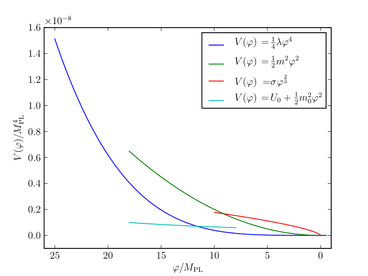
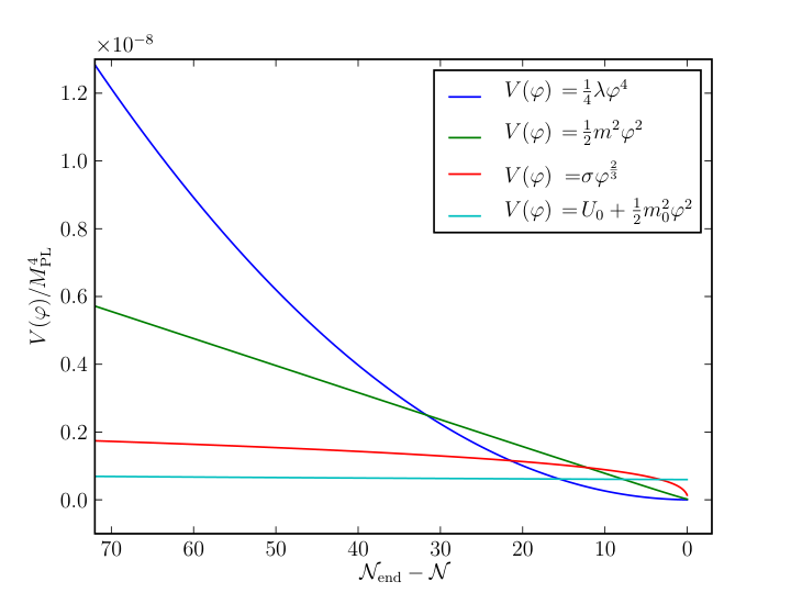
For each of the chosen potentials there is one free parameter that needs to be determined. We choose the parameters , , and so that calculated for each model is in agreement with the WMAP5 value at the pivot scale . The dependence of on each of the parameters can be seen in Figure 8. Requiring gives the values shown in Table 1. Here we have chosen the lower of the two possible values of shown in Figure 8d.
30.2 Initial Conditions
The background system requires initial conditions for and . These initial conditions and the range of e-foldings to be simulated must be selected with the choice of potential in mind. Not only must the e-folding range include an inflationary period, but the modes to be calculated at first and second order must begin inside the horizon. For example, the initial value for the model gives the background evolution described below and shown in Figure 9. As the evolution quickly reaches the attractor solution, the choice for is not particularly important; changing the initial value adds or subtracts a small number of e-foldings of evolution before the modes are initialised [165, 137].
The initial conditions are set for each mode a few e-foldings before horizon crossing. This follows Salopek et al.[169] and is justified on the basis that the mode is sufficiently far inside the horizon for the Minkowski limit to be taken. This initial time, , is calculated to be when
| (289) |
The range of e-foldings being used must include the starting point for all modes, but the parameter on the right hand side, here chosen to be 50, can be changed if needed. We use the small wavelength solution of the first order equations described in Section 3 as the initial conditions [169], with
| (290) | ||||
| (291) |
where conformal time can be calculated from
| (292) |
when changes slowly. For example is initialised about e-foldings before the end of inflation and crosses the horizon about e-foldings later. We also use these formulae in the calculation of the source term in Eq. (285) to determine the value of for a mode before its numerical evolution has begun.
We are interested in the production of second order effects by the evolution of the the Gaussian first order modes and we make no assumptions about the existence of second order perturbations before the simulation begins. Therefore, we set the initial condition for each second order perturbation mode to be at the time when the corresponding first order perturbation is initialised. One argument in favour of this choice of initial conditions is that far in the past the perturbations are assumed to be Gaussian and therefore the second (and higher) order perturbations would be identically zero.
A numerical solution for the second order perturbation equation will contain a homogeneous solution and a particular solution. The homogeneous part of the solution of the slow roll equation, Eq. (284), can be calculated analytically as done in Appendix 10.C. On their own the initial conditions we have chosen above do not remove this homogeneous solution from the result for in general. In order to do this, and keep only the particular solution to the equation, it is necessary to ensure that the homogeneous solution is the trivial solution throughout the evolution. We have not attempted to do this in this thesis but it is an important issue for further study in the future. Approaches to removing the homogeneous part of the solution include calculating a semi-analytic value for the second order initial conditions which equals the particular solution or numerically trying to select the trivial homogeneous solution by introducing a ramping function to the source term in Eq. (285). In summary, the results quoted in Chapter 8 for the second order perturbations include both a homogeneous and particular solution. Extraction of either of these parts from the full result remains an issue for future study.
31 Implementation
The current implementation of the code is mainly in the Python1616 16 Python website: http://www.python.org programming language (with compiled Cython components) and uses the Numerical and Scientific Python modules for their strong compiled array support [87]. The core of the model computation is a Runge-Kutta fourth order method (see, for example, Eq. (25.5.10) in [1]). Following Refs. [137] and [165], the numerical calculation proceeds in four stages. The background equation (282), rewritten as two first order equations, is evolved from the specified initial state until some end time required to be after the end of the inflationary regime. The end of inflation occurs when is no longer positive and the parameter becomes greater than or equal to unity (see Figure 9). This specifies a new end time for the first order run, although the simulation can run beyond the strict end of inflation if required. For the model, the end of inflation is set by hand to remove the need for a second, inflation-terminating field. The initial conditions for the first order system are then set as above.
The system of ordinary differential equations for the first order perturbations in Eq. (283) is integrated using a standard fourth order Runge-Kutta method. A fixed time step method is used in order to simplify the construction of the second order source term. This is also necessary since it is not known a priori which time steps would be required at second order if an adaptive time step system were used. The first order equations are separable in terms of and so it is straightforward to run the system in parallel and collate the results at the end. However, as will be discussed below, the first order calculation is not computationally expensive in comparison with the other stages and only takes of the order of a few minutes for around time steps with and modes.
Once the first order system has been solved, the source term for the second order system must be calculated. As the real space equation for the source involves terms quadratic in the first order perturbation, it is necessary to perform a convolution in Fourier space, as shown in Eq. (274). We do not transform back into real space due to the presence of both gradient operators and their inverses. Instead, the slow roll version of the source term integrand was used, although it is worth remarking that the method can also be applied to the full equation. This stage is computationally the most intensive, and can be run in parallel since the calculation at each time step is independent of the others. The nature of the convolution integral and the dependence of the first order perturbation on the absolute value of its arguments requires that twice as many modes are calculated at first order than are desired at second order. As the first order calculation is computationally cheaper than the source term integration, this does not significantly lower the possible resolution in -space, which is still limited by the source term computation time. Once the integrand is determined, it is fed into a Romberg integration scheme. As for , which was discretised by points in Eq. (273), this requires that the number of modes is
| (293) |
for some1717 17 The number of discretised modes does not need to be equal to .. This requirement can be relaxed by opting for a less accurate and somewhat slower standard quadrature routine.
The second order system is finally run with the source term and other necessary data being read as required from the memory or disk. The Runge-Kutta method calculates half time steps for each required point. For example, if is known and is required (for step size ), the method will calculate the derivatives of at and . As we need to specify the source term at every calculated time step, the requested time step for the second order method must be twice that used at first order. This decreases the accuracy of the method, but does not require the use of splines and interpolation techniques to determine background and first order variables between time steps.
The second order system is similar in run time to the first order system. However, the source integration is more complex and involves the integration of values at each time step. When and , the first order evolution lasts around 200 seconds. The source calculation, on the other hand, takes approximately 200 seconds for each time step. Each of the four terms is approximately 16 gigabytes in size at each time step for these values of and . However, only the integrated result is stored for use in the second order run. This is approximately kilobytes in size for each time step. Results for each stage are stored in the open HDF5 standard [9, 79], which can deal efficiently with large files, is very portable and allows for data analysis independent of the Python/Numpy programming environment.
The full calculation contains around 8000 time steps, making the source term calculation approximately 470 hours long. Each time step is independent of the others, however, so parallelisation of the system is straightforward. The results in Chapter 8 were obtained on the Virgo Cluster in the Astronomy Unit at Queen Mary, University of London. The code was run on ten nodes, each containing four Opteron cores with a clock speed of Mhz. With this configuration the run time of the source term calculation is reduced to under twelve hours.
32 Code Tests
The numerical code has been tested in a variety of controlled circumstances in order to quantify the effects of different parameter options. In particular, it is important to establish whether the values specified for the number of discretised ’s, , the size of the spacing of the discretised modes, , and the range of values significantly impact on the results. The sections of the code that solve ODEs are straightforward and follow standard algorithms.
As mentioned above, the WMAP results [104] use observations in the range . We will consider three different ranges both in our results and the tests of the code1818 18 The ranges in are: :
| (294) |
The first, , has a very fine resolution but covers only a small portion of the WMAP range. The next, , is closest to the WMAP range and still has quite a fine resolution. The final range, , has a larger mode step size, , and covers a greater range than the others. It extends to much smaller scales than WMAP can observe.
The central calculation in the code is of the convolution of the perturbations for the source term, Eq. (285). The first of the dependent terms in Eq. (273), , can be convolved analytically for certain smooth choices of . Taking to be similar in form to the initial conditions (290) gives with proportionality constant . If denotes the following integral of the term:
| (295) |
then substituting implies that
| (296) |
This has the analytic solution
| (297) |
The dependence of can be seen in Figure 10. We have tested our code against this analytic solution for various combinations of ranges and . The relative error
| (298) |
is small for all the tested cases, but certain combinations of parameters turn out to be more accurate than others. The relative errors of all the following results are not affected by the choice of so we will keep its numerical value fixed throughout as .
We first tested the effect of changing , the number of samples of the range . Figure 11a plots these results for the range with . Only three values of are shown for clarity. It can be seen that increasing decreases the relative error when the other parameters are kept constant, as one might expect.
As mentioned above the choice of range is especially important as the convolution of the terms depends strongly on the minimum and maximum values of this range. Indeed, this is clear from the analytic solution in Eq. (297). Figure 11b shows the difference in relative error for the three different ranges described above with and (), respectively. The accuracy is similar in all three cases.
Another important check is whether the resolution of the range is fine enough. Varying can not be done in isolation if the constraint (293) for is to be satisfied. For this test the end of the range was changed with but the other parameters were kept fixed at and . Figure 12 plots these results again for three indicative values. For , there is a marked degradation in the accuracy of the method for the upper two lines. This is understandable as many interpolations of multiples of below will be set to zero. Once is greater than , the relative error is insensitive to further increases in the value of . (This is not shown in the figure.)
The analytic solutions for the , and terms are given in Appendix 10.D. The relative errors between the analytic and calculated values for , and are shown in Figure 14 for the three final ranges, with . The errors for the and terms are very small, being of the order of and , respectively. The relative error for the term is larger, especially for small values. However, the error is still below for each of the , and ranges.
It should be noted that these tests only show the relative errors in the computation of integrals of the four terms in Eq. (273). They do not represent errors for the full calculation. However, they do show that the accuracy is good compared with the analytic result.
33 Discussion
This chapter has described the implementation of the numerical calculation of second order cosmological perturbations. The Klein-Gordon equations in Chapter 6 are the central focus of this computation. In Section 30 these equations were rewritten using as the time variable, a choice more suitable for numerical work. The convolution integrals in Eq. (259) can be expressed in spherical polar coordinates and split into four sub-terms – in Eqs. (273) and (286). Computing the source term Eq. (285), which is written using –, is the most complex and time consuming part of the calculation.
To demonstrate the numerical code, four different potentials have been chosen and these were described in Section 30.1. One parameter for each potential was determined by comparing the calculated with the WMAP5 value.
In Section 30.2 the initial conditions for the computed quantities were explained. Each mode is initialised well inside the horizon using the Bunch-Davies vacuum conditions from Section 3. The second order perturbations are initially set to zero. This choice concentrates focus on the generation of second order effects during the observable period of inflation.
The technical implementation of the code was discussed in Section 31. There are four stages in the procedure. First, the background fields are evolved over a specified time period. The end time of inflation is then determined by the condition and the scale factor calculated for this time. With this information the initialisation of the first order modes can be performed. In the second stage, the first order perturbation equations are solved. These results are used in the third stage to calculate the source term (285) at each time step and for each value. Finally, the second order perturbation equations are solved using the source term results.
To test the source term calculation the numerical results were compared to analytic solutions in Section 32. Numerical parameters such as and were set by minimising the relative error between the two approaches.
In Chapter 6 the evolution equations for second order perturbations were introduced. In this chapter the practical implementation of a numerical calculation of these perturbations was discussed. In Chapter 8 the results of this numerical calculation will be examined and the next steps towards an improved procedure will be described.
Chapter 8 Results and Future Work
34 Introduction
The main result of Part II of this thesis is the numerical integration of the Klein-Gordon equation of motion for second order scalar field perturbations, Eq. (259). The slow roll approximation of the source term for second order perturbations was employed, but the complete versions of the evolution equations were used for the background and first order perturbations. In this chapter the results of the numerical calculation will be presented. This represents the first step towards a full calculation of the Klein-Gordon equation at second order. In addition to the new results obtained, plans will be described for future work aimed at improving the numerical system and increasing its range of applicability.
As a proof of concept, the numerical system was tested with four different potentials, , , and , and results computed across three different ranges. As expected, the second order perturbation for a single, slowly rolling inflaton field that we have calculated is extremely small in comparison with the first order term. However, there are differences apparent between the potentials, which will be outlined in Section 35.3.
We have listed the potential parameters , , and in Table 1. These were found using the WMAP5 normalisation at [104]. We have also outlined in Eq. (294) the three ranges that have been used:
| (299) |
Many of the results will be quoted for which lies in all three of these ranges.
Given that the first order perturbations for the chosen potentials produce an almost scale invariant power spectrum with no running, it is no surprise that the results from the three different ranges are very similar. The second order source term is somewhat dependent on the lower bound of (upper bound on size). This is also to be expected and in the scale invariant case a logarithmic divergence can be shown to exist [124]. We have implemented an arbitrary sharp cutoff at , below which is taken to be zero. As mentioned in Chapter 7, there is some evidence to suggest that a similar cutoff might be supported by the WMAP data [187, 95].
In Section 35, the numerical results for the computation described in Chapter 7 are presented. Comparisons of the results from the four different test potentials will be made in Section 35.3. Since this represents the first stage towards a full calculation of the source term, the next steps that will be required are outlined in Section 36. Finally, in Section 37 we discuss some of the consequences of our results.
35 Results
35.1 Results for
At first order the solutions obtained for the quadratic potential agree with previous work in Refs. [169, 137, 165]. Oscillations are damped until horizon crossing (when ) after which the curvature perturbation becomes conserved. Figure 15 shows the evolution of the real and imaginary parts of the first order perturbation from when the initial conditions are set, at , to just after horizon crossing. The horizontal axis for most of the following figures parametrises the number of e-foldings remaining until the end of inflation (), instead of the time variable employed in the calculations.
Figure 16 shows the evolution of the second order perturbations for the scale . As mentioned above, the overall amplitude of the second order perturbation is many orders of magnitude smaller than the corresponding first order one. The results given for in this chapter are for the full solution which includes a homogeneous and particular solution as described in Section 30.2. In Figures 15 and 16 the field values have been rescaled by to allow for a better appreciation of the magnitude of the resulting power spectra.
The source term is calculated using Eq. (275) at each time step using the results of the first order and background simulations. This term drives the production of second order perturbations as shown in Eqs. (259) and (284). Figure 17a shows the absolute magnitude of the source term for a single mode, , for all time steps calculated. The source term is large at early times, and closely follows the form of the spectrum of the first order perturbations, as can be seen from Figure 17b.
Figure 18 shows how the source term depends on the choice of range. After horizon crossing, the source term is independent of the specific choice of (). Before horizon crossing, however, there is a strict hierarchy with the smaller ranges, and , leading to smaller source contributions. As discussed in Section 32, should be at least as large as in order for the error to be reduced to a minimum. In Figure 19 the source term is plotted at three different values of for the range . As increases, or equivalently the length scale decreases, the magnitude of the source term after horizon crossing decreases.
It is informative to compare the magnitude of the source term with the other terms in the second order evolution equation (284). We denote these other terms by :
| (300) |
Figure 20 then shows the absolute magnitude of both and . It is clear that for the scale the contributions to the source term are only of comparable magnitude during the early stages of the simulation. Figure 21 shows a comparison of for three different values. The magnitude of is closer to that of the rest of the terms for the larger mode. A priori, the range of modes where will be large for a particular chosen potential is not known. However, once the relevant values of have been determined, it may be possible to significantly reduce the time required for the simulation by restricting the calculation of to those regions where it is important. Figure 21 shows that it is not possible to arbitrarily ignore the contribution of either inside or outside the horizon. The full calculation on sub- and super-horizon scales is important for the evolution of the second order perturbation at different scales.
In Figure 22 the value of at the initialisation time for each mode is shown. The initial magnitude of the source term is much smaller for larger values of (smaller scales). Because the smaller modes begin their evolution earlier, the relative difference in is not as pronounced when measured at a single time step (see for example Figure 19). It should also be remembered that the magnitude of the other terms in the second order ODE is small for larger modes as shown by the ratio in Figure 21.
The source term can also be compared at different time steps over all the values. In Figure 23 the green line shows when all modes have started to evolve. The lower red line illustrates after all modes have exited the horizon, around 52 e-foldings before the end of inflation.
35.2 Comparison of Results with Analytic Solution
In this section results for the quadratic model will be compared with an analytic solution for this model. However, an analytical result is difficult to obtain for the case of the full first order solution in terms of Hankel functions with the phase information included. The analytical solution we will use, therefore, is the non-interacting de Sitter space solution with the phase information ignored. The first order perturbations are then given by
| (301) |
and the derivative in terms of is
| (302) |
The source term is found using Eq. (285) and the values of the background quantities. The analytical solution of Eq. (285) for this choice of first order solution is given in Appendix 10.E in Eqs. (357-364).
In Figure 24 the analytical and calculated solutions are plotted for one timestep about 60 e-foldings before the end of inflation. At a single time step the correlation between the two solutions for is very good. There is a deviation at small values of due to the analytical solution getting rapidly smaller as approaches zero. This is not replicated in the calculated version. However, this only strongly affects the result for the smallest values of and for for example the relative error of the calculated solution compared to the analytical solution is about . The relative error of the calculated solution is shown in Figure 25 for a single time step.
The analytical and calculated values for the source term can also be compared for a single value across a range of time steps. In Figure 26 the absolute magnitude of the source term for is plotted for a range of a few e-foldings before horizon crossing. The analytical and calculated results are extremely similar and not distinguishable in the plot. The relative error of the calculated solution is around . Because the first order perturbations do not include any phase information the result is much smoother than the result generated using the full first order phase information. However, as the phase angle is a function of it cannot be trivially ignored in the computation of the full convolution integral.
35.3 Comparison of Models
All the results quoted so far have been for the quadratic potential. In this section the results for all four potentials will be compared using the range.
Figure 27 shows the power spectrum of first order curvature perturbations, , for each potential. The , and models all clearly have a red spectrum with . On the other hand, the model has a blue spectrum () when to chosen to be , as specified in Section 30.1. The values of obtained for the four potentials are given in Table 2.
| Potential | ||
|---|---|---|
| 0.965 | -0.035 | |
| 0.949 | -0.051 | |
| 0.977 | -0.023 | |
| 1.002 | 0.002 |
The source term for each model is shown separately in Figure 28 for using the range1919 19 These plots use a different range to the ones comparing and in Ref. [84].. Although these terms are qualitatively similar, differences between them are apparent. Figure 29 brings together the source terms at to enable a direct comparison to be made. The mode begins at different times for the different models. Each result is therefore plotted in terms of the initialisation time for that mode. This change in duration is a consequence of allowing to evolve during the calculation.
The source term results for the quadratic and quartic potentials are very similar. Indeed, from horizon crossing to near the end of inflation the results appear to coincide. The mode has a slightly longer duration and at late times is reduced in comparison with the one. Figure 30 shows that at early times the relationship is more complicated with the mode being larger for a significant period.
In the early stages the amplitude of the model is very similar to the other two results described above. After horizon crossing, however, there is a significant drop in the amplitude of in comparison with the and models. This continues until late in the evolution when increases swiftly to reach levels above the others. The duration of the mode in this model is shorter than in the other two models described so far.
The fourth model, with potential , is a contrived toy model. As described in Section 30.1, in order to perform the single field calculation, the end time of inflation must be specified by hand. In this simulation is taken as the end time. The potential is extremely flat in this region and the effect of this can be seen in the source term of the model. Before horizon crossing it is of comparable magnitude to the other terms. However, a steep decrease in ensures that it is a few orders of magnitude smaller than the other terms after horizon crossing. In contrast to the behaviour of the other models, the source term does not increase close to the end of inflation. This is due to the enforced end time cut-off which means that does not become large.
In this section we have described the results for four different single field potentials. As expected for single field slow roll models they exhibit similar properties. In the next section plans to extend the calculation to deal with more interesting models will be outlined.
36 Future Directions
There are many possible ways to improve the program outlined in Chapter 7. Chief amongst these is the implementation of the full second order source term given in Eqs. (254) and (255). As we have seen the slow roll approximation is very helpful in reducing the equations of motion to a manageable size. However, many interesting models break the assumptions of a slowly rolling field and to investigate these models it is necessary to use the full field equations.
Models in which the field potential is not smooth due to the presence of a feature are particularly interesting examples of single field inflation for which slow roll is broken. As the derivatives of the potential can be large around the feature, these models must necessarily be handled without assumptions about the size of the slow roll parameters. In Ref. [3] a model with a step potential was proposed which takes the form
| (303) |
where , and parametrise the location, height and width of the step feature. A bump model has also been proposed [42], with potential
| (304) |
where again , and parametrise the feature. At first order these models introduce noticeable differences in the scalar power spectrum. They are also known to be able to produce significant amounts of non-Gaussianity in shapes which are not similar to either the local or equilateral types described in Section 6 [41, 42].
It will also be important to go beyond slow roll in the multiple field case. To obtain analytic results, the study of multi-field models has often been restricted to those with either sum or product separable potentials. Even very simple models with two fields such as the double inflation model with the potential given by [197, 184]
| (305) |
can violate slow roll when the fields and are close to equality. To go some way towards considering the full range of possible multi-field models with arbitrary inflationary potentials then requires that the full non-slow roll evolution equations are used.
As far as the implementation of the code is concerned, the extension to the non-slow roll single field case is the next step. Although clearly more complicated than the slow roll case of Eq. (284), only three more dependent terms need to be added to the – terms listed in Eq. (273). The four potentials considered above all result in slow roll inflation. Therefore, it is not expected that using the full source equation will result in an appreciably different outcome in these models until near the end of the inflationary phase. Once the field has stopped rolling slowly, new observable features are expected to arise, as is indeed the case at first order.
Eqs. (254) and (255) must be written in terms of , with the dependent terms grouped together, in order to set up the numerical system completely at second order. The main equation becomes
| (306) |
where the full source equation is given by
| (307) |
The term in Eq. (307) requires the use of three further integrals in addition to those presented in Eq. (273). These take the form
| (308) |
It is worth noting that the term tends to zero in the limit where and . The term can now be written in terms of , and :
| (309) |
Eqs. (307) and (309) are clearly more complicated than the slow roll versions used in Chapter 7. The numerical complexity is not significantly greater, however, once the three terms in Eq. (308) have been calculated. The running time of the full calculation will clearly be a significant constraint.
With this in mind, the performance of the numerical simulation could be improved by analysing the most time consuming processes and investigating what optimisations might be implemented. The current, perhaps inelegant, procedure will allow any performance improvements to be benchmarked for accuracy as well as for speed. As discussed above, was set to for the test runs. This provides good coverage of the WMAP range, but it is not clear whether it sufficiently approximates the integral to infinity for the source term. Logistical factors, including the running time and memory usage of the code, restrict the choice of . By optimising the routines for reduced memory and increased speed it is hoped that the range of scales can be extended and the resolution enhanced.
Beyond these considerations, the next significant step is to implement a multi-field version of the system. This would allow the investigation of models that inherently produce large second order perturbations. In Ref. [133] the second order Klein-Gordon equation for multiple fields was presented and upgrading the simulation to use these equations should be a straight-forward (if lengthy) process. Extending the current data-structures and routines to a fixed number of extra fields will increase the numerical complexity and the run-time of the code.
For example, let us suppose that the second order perturbations of two scalar fields, and , are to be calculated. Let denote the potential and its background value. As the coding environment we have used can easily handle arrays of variables, it is useful to write the equations in vector form. The following definitions will be used:
| (310) | ||||||||
| (311) |
In conformal time the Friedmann equation becomes
| (312) |
where denotes the transpose of . The background vector equation of motion is given by
| (313) |
where is the zero vector. The first order vector equation takes the form
| (314) |
where is the identity matrix.
We will outline the second order vector equation using the slow roll approximation. In the multi-field case there are many more slow roll parameters than in the single field scenario. Extending the definition of in Eq. (258) to two fields gives
| (315) | ||||
| (316) |
There are now four -type parameters corresponding to the different combinations of second derivatives of . These can be written together in matrix form as
| (317) |
where . The magnitude of is only small in the adiabatic direction, so terms including are included when making the slow roll approximation [133].
The second order, slow roll, vector equation for the perturbations is given by
| (318) |
where the slow roll source term equation is
| (319) | ||||
| (320) |
Following the method of Section 30, the integral is evaluated and the integral is written in spherical polar coordinates. The dependent terms, which are equivalent to Eq. (273) in the single field case, are given by
| (321) |
The first two equations are not vector equations but are needed for the explicit matrix term in Eq. (319). We rewrite that equation with these definitions to obtain:
| (322) |
This expression for reduces to Eq. (275) when only one field is considered. At least in the slow roll case, the multi-field source term equation is not considerably more complex than the single field one. The extra numerical complexity arises from the calculation of the new dependent terms in Eq. (321).
37 Discussion
Part II of this thesis has described the numerical solution of the evolution equations for second order scalar perturbations. The closed form of the Klein-Gordon equation (259) has been employed for the first time. We have shown that direct calculation of the field perturbations beyond first order using perturbation theory is readily achievable, although it is non-trivial.
This first demonstration has been limited to considering the slow roll approximation of the source term in Eq. (259) which is quadratic in first order perturbations. Slow roll has not been imposed on the background or first order equations. Four different potentials were used to demonstrate the capabilities of the system. The singularity at , which arises as larger and larger scales are considered, is avoided by implementing a cutoff at small wavenumbers below . This is a pragmatic choice necessary for the calculation. It is also necessary to specify a maximum value of . This choice is dictated by computational resources and with reference to observationally relevant scales. In this demonstration, ranges have been used which are comparable with the scales observed by the WMAP satellite. By comparing the analytical results of the convolution integral with the numerical calculation, values of the parameters and were chosen in such a way that the numerical error was minimised. The convolution scheme that has been implemented works best when .
We have seen explicitly that the second order calculations for the chosen potentials can be completed once the cut-off for is imposed. As expected for these potentials the magnitude of second order perturbations is extremely suppressed in the slowly rolling regime, in comparison with the first order amplitude. We have also shown that the evolution of the source term during the inflationary regime can be readily calculated.
By computing the perturbations to second order, we have direct access to the non-Gaussianity of . When used to investigate models that predict a large non-linearity parameter, , this technique could yield greater insight into the formation and development of the non-Gaussian contributions by studying the effects of the different terms in the source equation (285). It was shown recently that can be calculated directly from the field equations [149, 175], instead of using the standard method based on a Lagrangian formalism [130]. The method presented here will therefore eventually allow a full numerical calculation of to be made.
Our numerical code evolves the second order perturbation itself and gives an insight into how this field behaves through the full course of the inflationary era. This is in contrast to other approaches which only consider the result for the three point function of the field, or alternatively of the curvature perturbation. The computational system handles perturbations with scales both inside and outside the horizon. Any effects of horizon crossing are visible and no assumptions need to be made about the form of the solution inside the horizon.
The numerical code, when developed with the full equation, will not require any simplifying assumptions about the form of the potential used. This allows models which are not amenable to analytic analysis to be examined. Examples of models which require consideration beyond the slow roll approximation include single field models with a step or other feature in the potential, and multi-field double inflation models where the field values are roughly equal.
The code we have developed is also applicable in other physical circumstances. Beyond scalar perturbations the form of the source term is similar in other interesting cosmological physics. The generation and evolution of non-Gaussian curvature perturbations is, of course, directly related to the behaviour of the second order scalars as has been described in Section 6 and Section 27. Investigating and classifying non-Gaussian signatures for inflationary models is the main goal of our future work.
The generation of vorticity in a cosmological setting has physical parallels with the equations we have studied. This second order effect arises through the vector perturbations which we have not considered in this thesis. Vorticity in the early universe could also lead to the generation of primordial magnetic fields, an area which is of increasing interest [48, 29]. The wave equations for tensor mode perturbations also exhibit the same form as the scalar equations with a source term at second order. The code we have developed could be modified to examine the behaviour of gravitational waves in the early universe at second order.
In summary, we have demonstrated that numerically solving the closed Klein-Gordon equation for second order perturbations is possible. The slow roll version of the source term was used in the calculation, but as described in Section 36, the extension of the system to include the full source term is achievable. The analytic and numerical solutions for the convolution terms were compared directly and found to be in good agreement. The models used have been shown to have negligible second order perturbations in line with known analytic results.
Part III Conclusion
Chapter 9 Conclusion and Discussion
As the number of viable cosmological models increases, the need to constrain them becomes more important. At the same time, the quantity and quality of observational data continue to improve. There now exists the opportunity to go beyond linear statistical analyses and confront the predictions of models with observational data from the non-linear regime. In this thesis both analytic and numerical methods have been developed to constrain inflationary models.
The framework used in this thesis is the Friedmann-Robertson-Walker universe, reviewed in Chapter 2. During the accelerated expansion of the inflationary period, quantum fluctuations seeded energy density variations, which in turn gave rise to the diverse structure of the present universe. First order cosmological perturbation theory is necessary to describe the evolution of these fluctuations. The main observable quantities can be calculated at horizon crossing by using the Bunch-Davies vacuum initial conditions. The departure of the perturbations from a purely Gaussian random field is parametrised by , which is described in two limits, local and equilateral. In addition to canonical actions, we also introduced non-canonical models, for which the speed of sound of the perturbations plays a crucial role. When the sound speed is small, the amplitude of for these models is large.
In Part I, analytic methods were developed to constrain string theory inspired non-canonical inflationary models. The Dirac-Born-Infeld scenario was outlined in Chapter 3. In this model, a D3-brane propagates in a six-dimensional warped throat. The radial position of the brane from the tip of the throat assumes the role of the inflaton field. The non-canonical nature of the DBI action restricts the kinetic energy of this field no matter how steep the potential. This allows an inflationary period of sufficient duration to occur. This model has been widely regarded as a very promising realisation of an inflationary model in a string-theory context.
In Ref. [19], Baumann & McAllister used the Lyth bound [123] to limit the tensor-scalar ratio. Their analysis was based on the conservative assumption that the brane could not propagate further than the full length of the throat. In Chapter 4, we showed that this bound can be tightened by applying it over the portion of the throat through which the brane passes during the directly observable stage of inflation. Restricting the field variation to be over these approximately four e-foldings constrains to be less than for standard parameter values.
The most optimistic estimates of advances in experimental techniques and data analysis, including foreground reduction, indicate that observations of might be achievable in the future [21, 199]. Therefore, the new bound in Eq. (136) immediately rules out the observation of a tensor mode signal from this model.
In addition to this, we also derived a lower bound on in Eq. (144). This depends on observable quantities, namely the scalar spectral index and the equilateral non-Gaussianity. Saturating the WMAP5 observational limit on and taking the best fit value for , we found that the most conservative lower limit is . This is clearly incompatible with the previously derived upper bound. Therefore, for standard parameter values, the D3-brane DBI scenario is not viable. Numerical simulations by Peiris et al.in Ref. [154] have demonstrated the lower bound, in the relativistic limit, using the Hamiltonian flow approach.
In Section 16, a phenomenological approach was taken to easing the upper bound on the tensor-scalar ratio. By considering a DBI-type action with unspecified field functions, , we showed that the generalised lower and upper bounds can be consistent if the product of and is sufficiently large on observable scales. This provides a guide to the types of models which could evade the inconsistency of the bounds on . For more general models with a non-canonical action, a bound on which relates the geometry of the throat, the number of e-foldings of observable inflation, and the derivatives of the action has been derived in Eq. (163). This bound, although it does not in general relate to observational quantities can be used when the details of a particular physical model are known.
The discovery of the incompatible bounds on for DBI inflation has had a noticeable impact on the research community, spurring interest in finding models which evade these bounds. Many such models have been proposed with varying degrees of success. In Section 17 these were categorised according to whether they featured single or multiple fields, and single or multiple branes. Some of these models are still constrained by the bounds on but not to the same extent as the standard DBI scenario. For example the parameter space of the models with wrapped brane configurations is still extremely limited by the observational values from WMAP5 [4]. For other models an analysis in terms of the bounds derived in this thesis has yet to be undertaken. As the observational limits on and continue to improve, an important step in ensuring the validity of DBI based models is to check whether equivalent bounds to those derived here exist, and whether they can be met for any significant proportion of the parameter space.
General actions which relax the bounds on , were derived in Chapter 5. We found a class of actions similar in form to that of the DBI model. However, instead of a square-root in the kinetic term, the index of the main term of these actions depends on the constant of proportionality between and the sound speed of inflaton fluctuations. The upper bound on can be derived for these general actions and when the index is below the critical value of (corresponding to the standard DBI scenario), this bound is significantly relaxed. When new models are proposed in the future, our phenomenological derivation of this family of actions will allow those models for which the bound on is less stringent to be easily identified.
One such model is the single field, multi-coincident brane scenario of Thomas & Ward [194]. When D3-branes propagate in a throat, the non-Abelian interactions between the branes result in major departures from the single brane case. This is in contrast to the non-interacting branes model, in which the total action is simply the sum of copies of the single brane action.
In the limit of a large number of branes being coincident, the effective action is similar to times the single brane model, with the addition of a fuzzy potential term. Indeed this model is of the type considered phenomenologically in Section 16 and the bounds derived in that section can be applied. These bounds on can be somewhat relaxed when this potential is large, but the model is still strongly constrained by current observations. For an throat, standard parameter choices limit the number of allowed branes to be less than 150, at which point the assumption of arbitrarily large becomes questionable.
More promising is the finite limit of the coincident brane model. The non-Abelian nature of the interactions leads, in this case, to a recursive relation for the -brane action in terms of the one. In Section 23, we showed that the action for finite is one of the class of bound-evading actions described above. This identification is possible because the last term of the recursive sum dominates in the relativistic limit. This approximation is valid at least when and the backreaction of the multiple branes is kept well under control for this range of .
Although the bounds on are eased for this model, we showed that observations strongly constrain the possibility of an observable tensor signal being generated. If an observable tensor-scalar ratio is considered to be , then only the two or three brane cases are capable of producing such a signal. This bound on depends on the WMAP5 limit on . If, as expected, the observational limits on tighten considerably in the future, the possibility of an observable tensor signal from the multi-coincident brane model could be ruled out.
On the other hand, the choice of as the threshold of an observable signal is very optimistic. If foreground removal techniques and the signal-to-noise ratios of future experiments cannot reach this threshold, and instead reach , no number of branes will be able to produce an observable tensor signal when combined with the current limits on the non-Gaussianity. There will then be little possibility of a distinguishing observational signature for these coincident brane models.
In Part II of this thesis, numerical methods were used to test inflationary models up to second order in cosmological perturbation theory. The Klein-Gordon equation at second order was derived in Ref. [133] for the multi-field case. In Chapter 6, second order gauge transformations were outlined and the Klein-Gordon equation reproduced for a single scalar field model. In contrast to the approach, this equation is valid on all scales, both inside and outside the horizon.
In Fourier space, the second order Klein-Gordon equation (254) contains a convolution term of the first order scalar field perturbation. For this first demonstration of the numerical system, a slow roll approximation of the full equation was used.
Calculating the second order scalar field perturbations provides the possibility of a unique insight into the generation and evolution of non-linear contributions to the scalar curvature perturbation. One advantage of using the inflaton field equations is that we can directly investigate how the perturbations are generated. If, instead, we integrated the evolution equation for a derived observable quantity, there would be a degree of separation from the physical origins of this process. Indeed, there is, as yet, no known evolution equation for the main observable quantity, the comoving curvature perturbation, at second order. Using cosmological perturbation theory also provides control over the calculation. The domain of applicability of the perturbative expansion is well defined and the resultant equations are certain to be valid in this domain.
The main observable quantity is not however the second order scalar perturbation, but rather the departure from Gaussianity in the CMB temperature map, parametrised by the amplitude of the bispectrum of the perturbations. In Section 27 we outlined how could be calculated from the numerically found both for the local type and more generally using the bispectrum of the uniform density curvature perturbation. As the observational limits on are tightened over the course of the remaining WMAP releases and future Planck data, the importance of comparing the predictions for of inflationary models with the observed values will only increase. In this thesis we have not computed for the models we have considered, but this is an important future step that will be undertaken.
The long term aim of this continuing project is to analyse multi-field, non-slow roll models, in which non-Gaussian effects are expected to play an important role. As a step towards this goal, we described the implementation of a numerical calculation of the single field, slow roll, second order equation in Chapter 7. The construction and evaluation of the convolved source term in Eq. (275) proved to be the most numerically complex step required.
To allow a numerical calculation, an energy scale cutoff must be implemented. We used a sharp cutoff at small wavenumbers below which the perturbations were taken to be identically zero. Another cutoff at small scales (or equivalently large wavenumbers) was dictated by practical considerations of calculation size and computation time.
We defined, in Eq. (273), four dependent integrals into which the convolution term can be decomposed. By comparison with an analytic solution for a particular smooth choice of the first order perturbation, an estimate was made of the relative error present in the integration of each term. The number of discrete wavenumber values, their spacing, and the number of discrete values were chosen to minimise the error in one of the integrals. From these parameter values, three different finite ranges of discrete values of the wavenumber were defined. These all contain the WMAP pivot scale at and cover the WMAP observed scales to varying degrees. Despite the ranges having being chosen to minimise the relative error in the integral of only one of the dependent terms, the integrals of the three other terms also display small relative errors for these ranges. The analytic solutions which have been found will form an important part of the verification of any future modifications to the numerical code.
The execution of the code is in four stages, building on previous calculations of first order perturbations in Refs. [137, 165, 169]. To begin, the background equations are solved and the end time of inflation is fixed. The initial conditions for the first order perturbation can then be set and solutions found for the evolution equations. Despite the large volume of calculations required at each time step, the easily parallelisable nature of the source term calculations allows the run time of the third stage to be reduced significantly. The final stage of the calculation uses the source term results to solve the second order perturbation equations.
The initial conditions for the second order perturbations are taken to be and as described in Section 30.2. For this choice of initial conditions the homogeneous part of the solution of the second order equation is zero at all times. As the perturbations are supposed to become more Gaussian the further back in time they are considered, in the limit of the far past the second order perturbations should be zero. It remains to be investigated whether the choice of initialisation time is sufficiently far in the past for this assumption to be accurate. At first order it is known that the perturbations are well approximated by the Bunch-Davies vacuum initial conditions even just a few e-foldings before horizon crossing. However, this choice of initialisation time may not be the most appropriate for the second order perturbations. In future work it would be worth considering whether the analytic Green’s function solution for at very early times could be integrated until the numerical initialisation time and used as the initial condition for the perturbation.
To test the code, four different, large field, monomial potentials were used. These were the standard quadratic and quartic potentials, a fractional index potential derived from the monodromy string inflation model and a toy model in which inflation is stopped by hand and a blue spectrum is produced. Each potential depends on a single parameter, which was fixed by comparing the resultant scalar curvature power spectrum with the WMAP5 normalisation. The slow roll approximation can be applied to all four potentials. These potentials are not meant to represent an exhaustive survey of single field slow roll models but are sufficiently different to exhibit different power spectra and second order source terms.
We presented the results for each potential in Chapter 8. The first order results match those in Refs. [137, 165, 169]. The results of the source term calculation show that before horizon crossing, the source term amplitude decays rapidly for all four potentials. The amplitude changes less after horizon crossing, until later times when it increases as the slow roll approximation breaks down.
The four different potentials have similar amplitudes before horizon crossing but reach different values after horizon crossing. The differences in the slow roll parameters for each potential are compared with the source term values in Appendix 10.F. The slow roll parameters do not appear to be directly related to the amplitudes of the source terms, at least in a linear fashion.
The choice of wavenumber range affects the amplitude of the source term, as expected, due to the implementation of a sharp cutoff at large scales. This dependence is only apparent, however, before horizon crossing. For a particular range, the magnitude of the source term decreases as wavenumber increases. However, the ratio of the source term to the other terms in the Klein-Gordon equation increases with wavenumber.
As expected, the amplitude of the second order scalar perturbations is much smaller than that of the first order ones. After the generation of the second order perturbations at early times, their evolution is that of a damped harmonic oscillator similar to the first order evolution.
We have shown that the magnitude of the source term can be important throughout the full evolution and that it is not sufficient to calculate this term only for modes either entirely inside or outside the horizon, i.e., taking a short or long wavelength approximation respectively. We have been able to access both of these regimes, by solving the evolution equations of the inflaton field perturbation. This is in contrast to other approaches which could have been taken, for example using the formalism, which is only applicable in the large scale limit.
The construction of any numerical code involves a considerable commitment of time and resources so it is important to understand why such an endeavour has been undertaken. The numerical calculation of first order cosmological perturbations is an invaluable part of the cosmologist’s toolkit. It allows analytic predictions of inflationary models to be confirmed where these exist, but also generates predictions where no analytic solution is possible. Another important use is to test predictions based on the slow roll approximation against the full evolution equations. We have taken the first step towards upgrading this standard numerical calculation to include second order scalar perturbations. The ability to check the predictions of inflationary models at second order will be a powerful tool to constrain these models and check the consistency of any analytic assumptions that have been made. Solving the inflaton field equations provides the most direct access to the non-linear effects that the increase in available statistics have made observationally important.
We have presented the first numerical calculation of the Klein-Gordon equation for second order scalar perturbations which was derived in Ref. [133]. Although we have restricted ourselves in this thesis to the single field, slow roll version of the second order equation, the expertise gained and the lessons learned in the development of the numerical system will be of significant assistance when the next steps towards a full multi-field calculation are taken.
In the past, a numerical calculation on the scale we have achieved would have been the preserve of dedicated super-computing facilities. We have demonstrated that a calculation of this scope is now possible using relatively modest local resources. If the computational power available increases, the practical limits on the resolution and extent of the ranges will ease. Further improvements in the efficiency of the code will also loosen these constraints.
Another consideration in the development of a numerical system is the possibility of code re-use. One of our future goals is to develop our code into a numerical toolkit which can be applied to a variety of physical situations. The equations of motion of the inflaton scalar field are similar in form to the governing equations of other important cosmological phenomena. Therefore, it should be possible to adapt the numerical system we have constructed and apply it to other areas of interest. The form of the second order equation and source term are similar to those applicable in the evolution of tensor perturbations and the generation of vorticity in the early universe. The flexibility of the numerical system we have developed will be a positive factor in any attempt to apply our code to these physical systems.
The numerical calculation described is the first step towards a system capable of handling the multi-field, non-slow roll models for which non-linear contributions are important. In Section 36, the next steps towards this goal were outlined. Continuing our work by calculating the second order perturbations for both the non-slow roll, single field case and the slow roll, multi-field case will pave the way for the eventual calculation of the non-slow roll, multi-field equations.
The full single field, non-slow roll, second order equation can be treated using the method already described. Three more dependent terms are necessary to compute the full convolution integral in this case. It will be important to find analytic solutions for these three extra terms, as already done for the terms in the slow roll case, in order to gauge the effectiveness of the extended code. When the extension to non slow-roll models is complete, it will be possible to investigate models with a step or other feature in their potential. These models can exhibit large amounts of non-Gaussianity produced around the feature with a shape dependence that is more general than that of the local and equilateral forms.
The Klein-Gordon equation for the multi-field case introduces further complexity. We plan to expand the numerical system to encompass two or three scalar fields. The differences between single and multi-field models are already apparent for these cases. We have presented the slow roll source term equation for multiple fields in vector notation. The definitions of the four dependent terms used in the single field, slow roll model were also extended to the multi-field case. Beyond the slow roll approximation, the full multi-field equation should be treatable in a similar manner to the single field case, by introducing further dependent terms.
To conclude, it is worth reiterating our opening remarks. Cosmology has moved from being a theorists’ playground to a genuine scientific discipline. Inflationary models can now be strongly tested by observations and the next generation of experiments will place even tighter limits on the viable parameter space of such models. In this thesis, analytic arguments have constrained string theory inspired inflationary models and numerical methods have paved the way to calculating higher order cosmological perturbations.
Chapter 10 Appendix
The following materials supplement the calculations and discussions in the main thesis.
Appendix 10.A Analytic Solution of Generalised Sound Speed Relation
Eq. (169) can be analytically solved in full generality without imposing the limits (171) on the derivatives of the kinetic function. This allows us to determine the most general class of models where the non-linearity parameter satisfies the condition at leading order.
In general Eq. (169) takes the form
| (323) |
and this reduces to
| (324) |
where . Eq. (324) can be transformed into the linear equation
| (325) |
after the change of variables and the general solution to Eq. (325) is given by
| (326) |
Integrating a second time implies that
| (327) |
where and we have redefined the arbitrary integration functions . Finally Eq. (327) can be formally integrated in terms of a hypergeometric function
| (328) |
which represents the most general solution for this class of models. Note that we have set the remaining constant of integration to zero to ensure that the kinetic function vanishes in the limit of zero velocity. In fact this expression admits many different classes of solution, arising as limits of the expansion of the hypergeometric function.
Appendix 10.B Generalised BM bound for Finite Models
For completeness we should also consider the BM bound (157) for the finite multi-coincident brane models. This is given by
| (329) |
and in the case of an throat simplifies to
| (330) |
Comparing the limits in Eqs. (231) and (330) implies that the bound (163) is stronger than the corresponding BM bound (157) if
| (331) |
and this condition is always satisfied if
| (332) |
Moreover, the bound (332) will itself be satisfied for all values of and if it is satisfied when the limits and are imposed. Hence, we conclude that the bound (163) is stronger for . In general, it is difficult to quantify the magnitude of without imposing further restrictions on the parameters of the models and, in particular, on the functional form of the inflaton potential. However, if the ratio remains approximately constant during the final stages of inflation, one would anticipate that . Nevertheless, if , the bound (331) will only be violated for if .
Appendix 10.C Discussion of Homogeneous Solution for Second Order Equation
The homogeneous equation for the second order perturbations is
| (333) |
During slow roll, with the slow roll variables and defined in Chapter 2, this becomes
| (334) |
If we let , this equation can be rewritten as
| (335) |
When is small, the conformal time is given by
| (336) |
so we can rewrite Eq. (335) as
| (337) |
If the derivatives are taken in terms of instead of this is in the form of a Bessel equation with solutions in terms of Hankel functions given by
| (338) |
where are the Hankel functions (Bessel functions of the third kind), and is given by
| (339) |
The full solution for is then
| (340) |
where . When the (real) argument of the Hankel functions goes to they have the following asymptotic form [1]:
| (341) | ||||
| (342) |
So at early times when and we have the following expressions for u:
| (343) | ||||
| (344) |
where we have assumed that is slowly varying far in the past, i.e., the derivatives of the slow roll parameters are very small.
As explained in Section 30.2, the results given for are for the full solution including the homogeneous part. To remove the homogeneous part of the solution the initial conditions for the full should be chosen such that at all times.
Appendix 10.D Analytic Tests for and Terms
Analytic solutions can also be found for the , and terms. The term integral, , is given by
| (346) |
and has the following analytic solution when :
| (347) |
If, in addition to , we also take
| (348) |
then the and terms can be integrated analytically. The integral of the term is
| (349) |
and the analytic solution is given by
| (350) |
The integral of the term is
| (351) | ||||
| (352) |
and the analytic solution is
| (353) |
Appendix 10.E Analytic Solution for Source Term
Suppose the first order perturbations are given by the non-interacting de Sitter space solution such that
| (354) |
and the derivative in terms of is
| (355) |
The analytic solution of Eq. (285) for this choice of first order solution can be written in terms of four integrals of the - terms:
| (356) |
where
| (357) | ||||
| (358) | ||||
| (359) | ||||
| (360) |
The analytic solution for is given by
| (361) |
The analytic solution for is
| (362) |
The analytic solution for is
| (363) |
The analytic solution for is
| (364) |
Appendix 10.F Discussion of properties of source term for different potentials
The evolution of the source term for the four potentials has been discussed in Section 35.3, with particular emphasis on the evolution after horizon crossing as shown in Figure 29. Here the differences apparent at early times, shown in Figure 30 are commented on.
At early times the first order perturbations are still very close to the Bunch-Davies initial conditions as outlined in Section 30.2. In particular the perturbations are highly oscillatory with phase , where is the conformal time. When is small this is given by
| (365) |
It is therefore instructive to plot the slow roll parameter for the four potentials at these early times, as has been done in Figures 31 and 32. For completeness the other slow roll parameter defined in Eq. (27) has been plotted in Figures 33 and 34.
Figures 31 and 33 show and for the four different models. Figures 32 and 34 show the early stages of the evolution as in Fig 30.
As is clear from these figures the change in the slow roll parameters is not easily related to the differences in the profiles of the four potentials in Figure 30. In particular, although and are quite different for the quadratic and quartic models, the magnitude of after horizon crossing for these models is very similar.
At the earliest stages of the calculation of , one or two e-foldings after the initialisation of the first order perturbation, there appear to be small oscillations which affect the models in different ways. The highly oscillatory initial conditions, combined with the small but appreciable differences in and contribute to this effect. In Figure 35 the real part of the phase of the initial condition for is plotted just after initialisation for the four potentials. The small differences in phase for each model combined with the sharp cutoff at large and small values could explain the variations in at early times as seen in Figure 30.
References
- [1] Abramowitz M. and Stegun I.A., Handbook of Mathematical Functions with Formulas, Graphs, and Mathematical Tables. Dover, New York, 1964.
- [2] Acquaviva V., Bartolo N., Matarrese S., and Riotto A., “Second-order cosmological perturbations from inflation,” Nucl. Phys. B667 (2003) 119–148, arXiv:astro-ph/0209156.
- [3] Adams J.A., Cresswell B., and Easther R., “Inflationary perturbations from a potential with a step,” Phys. Rev. D64 (2001) 123514, arXiv:astro-ph/0102236.
- [4] Alabidi L. and Lidsey J.E., “Single-Field Inflation After WMAP5,” Phys. Rev. D78 (2008) 103519, arXiv:0807.2181 [astro-ph].
- [5] Albrecht A. and Steinhardt P.J., “Cosmology for grand unified theories with radiatively induced symmetry breaking,” Phys. Rev. Lett. 48 (1982) 1220–1223.
- [6] Alexander S., Biswas T., Notari A., and Vaid D., “Local Void vs Dark Energy: Confrontation with WMAP and Type Ia Supernovae,” JCAP 0909 (2009) 025, arXiv:0712.0370 [astro-ph].
- [7] Alishahiha M., Silverstein E., and Tong D., “DBI in the sky,” Phys. Rev. D70 (2004) 123505, arXiv:hep-th/0404084.
- [8] Alnes H., Amarzguioui M., and Gron O., “An inhomogeneous alternative to dark energy?,” Phys. Rev. D73 (2006) 083519, arXiv:astro-ph/0512006.
- [9] Alted F., Vilata I., et al., “PyTables: Hierarchical datasets in Python.” http://www.pytables.org/, 2002–.
- [10] Arroja F., Mizuno S., and Koyama K., “Non-Gaussianity from the bispectrum in general multiple field inflation,” JCAP 0808 (2008) 015, arXiv:0806.0619 [astro-ph].
- [11] The SNLS Collaboration, Astier P. et al., “The Supernova Legacy Survey: Measurement of , and from the First Year Data Set,” Astron. Astrophys. 447 (2006) 31–48, arXiv:astro-ph/0510447.
- [12] Avgoustidis A. and Zavala I., “Warped Wilson Line DBI Inflation,” JCAP 0901 (2009) 045, arXiv:0810.5001 [hep-th].
- [13] Babich D., Creminelli P., and Zaldarriaga M., “The shape of non-Gaussianities,” JCAP 0408 (2004) 009, arXiv:astro-ph/0405356.
- [14] Bachas C., Douglas M.R., and Schweigert C., “Flux stabilization of D-branes,” JHEP 05 (2000) 048, arXiv:hep-th/0003037.
- [15] Bardeen J.M., “Gauge Invariant Cosmological Perturbations,” Phys. Rev. D22 (1980) 1882–1905.
- [16] Barnaby N. and Cline J.M., “Non-Gaussian and nonscale-invariant perturbations from tachyonic preheating in hybrid inflation,” Phys. Rev. D73 (2006) 106012, arXiv:astro-ph/0601481.
- [17] Bartolo N., Komatsu E., Matarrese S., and Riotto A., “Non-Gaussianity from inflation: Theory and observations,” Phys. Rept. 402 (2004) 103–266, arXiv:astro-ph/0406398.
- [18] Baumann D., “TASI Lectures on Inflation,” arXiv:0907.5424 [hep-th].
- [19] Baumann D. and McAllister L., “A Microscopic Limit on Gravitational Waves from D-brane Inflation,” Phys. Rev. D75 (2007) 123508, arXiv:hep-th/0610285.
- [20] Baumann D. and McAllister L., “Advances in Inflation in String Theory,” arXiv:0901.0265 [hep-th].
- [21] CMBPol Study Team Collaboration, Baumann D. et al., “CMBPol Mission Concept Study: Probing Inflation with CMB Polarization,” AIP Conf. Proc. 1141 (2009) 10–120, arXiv:0811.3919 [astro-ph].
- [22] Bean R., Chen X., Peiris H., and Xu J., “Comparing Infrared Dirac-Born-Infeld Brane Inflation to Observations,” Phys. Rev. D77 (2008) 023527, arXiv:0710.1812 [hep-th].
- [23] Bean R., Shandera S.E., Henry Tye S.H., and Xu J., “Comparing Brane Inflation to WMAP,” JCAP 0705 (2007) 004, arXiv:hep-th/0702107.
- [24] Becker M., Leblond L., and Shandera S.E., “Inflation from Wrapped Branes,” Phys. Rev. D76 (2007) 123516, arXiv:0709.1170 [hep-th].
- [25] Bennett C.L. et al., “Cosmic temperature fluctuations from two years of COBE differential microwave radiometers observations,” Astrophys. J. 436 (1994) 423–442, arXiv:astro-ph/9401012.
- [26] Bennett C.L. et al., “4-Year COBE DMR Cosmic Microwave Background Observations: Maps and Basic Results,” Astrophys. J. 464 (1996) L1–L4, arXiv:astro-ph/9601067.
- [27] Bernardeau F. and Uzan J.P., “Non-Gaussianity in multi-field inflation,” Phys. Rev. D66 (2002) 103506, arXiv:hep-ph/0207295.
- [28] Berndsen A., Lidsey J.E., and Ward J., “Non-relativistic Matrix Inflation,” arXiv:0908.4252 [hep-th].
- [29] Biermann L., “Über den Ursprung der Magnetfelder auf Sternen und im interstellaren Raum (miteinem Anhang von A. Schlüter),” Zeitschrift Naturforschung Teil A 5 (1950) 65–+.
- [30] Brodie J.H. and Easson D.A., “Brane inflation and reheating,” JCAP 0312 (2003) 004, arXiv:hep-th/0301138.
- [31] Brummer F., Hebecker A., and Trincherini E., “The throat as a Randall-Sundrum model with Goldberger-Wise stabilization,” Nucl. Phys. B738 (2006) 283–305, arXiv:hep-th/0510113.
- [32] Bruni M., Matarrese S., Mollerach S., and Sonego S., “Perturbations of spacetime: Gauge transformations and gauge invariance at second order and beyond,” Class. Quant. Grav. 14 (1997) 2585–2606, arXiv:gr-qc/9609040.
- [33] Burgess C.P., Cline J.M., Stoica H., and Quevedo F., “Inflation in realistic D-brane models,” JHEP 09 (2004) 033, arXiv:hep-th/0403119.
- [34] Burgess C.P., Majumdar M., Nolte D., Quevedo F., Rajesh G., and Zhang R.J., “The Inflationary Brane-Antibrane Universe,” JHEP 07 (2001) 047, arXiv:hep-th/0105204.
- [35] Butti A., Grana M., Minasian R., Petrini M., and Zaffaroni A., “The baryonic branch of Klebanov-Strassler solution: A supersymmetric family of SU(3) structure backgrounds,” JHEP 03 (2005) 069, arXiv:hep-th/0412187.
- [36] Cai Y.F. and Xia H.Y., “Inflation with multiple sound speeds: a model of multiple DBI type actions and non-Gaussianities,” Phys. Lett. B677 (2009) 226–234, arXiv:0904.0062 [hep-th].
- [37] Cai Y.F. and Xue W., “N-flation from multiple DBI type actions,” Phys. Lett. B680 (2009) 395–398, arXiv:0809.4134 [hep-th].
- [38] Chen X., “Inflation from warped space,” JHEP 08 (2005) 045, arXiv:hep-th/0501184.
- [39] Chen X., “Multi-throat brane inflation,” Phys. Rev. D71 (2005) 063506, arXiv:hep-th/0408084.
- [40] Chen X., “Running Non-Gaussianities in DBI Inflation,” Phys. Rev. D72 (2005) 123518, arXiv:astro-ph/0507053.
- [41] Chen X., Easther R., and Lim E.A., “Large non-Gaussianities in single field inflation,” JCAP 0706 (2007) 023, arXiv:astro-ph/0611645.
- [42] Chen X., Easther R., and Lim E.A., “Generation and Characterization of Large Non-Gaussianities in Single Field Inflation,” JCAP 0804 (2008) 010, arXiv:0801.3295 [astro-ph].
- [43] Chen X., Huang M., Kachru S., and Shiu G., “Observational signatures and non-Gaussianities of general single field inflation,” JCAP 0701 (2007) 002, arXiv:hep-th/0605045.
- [44] Chen X. and Tye S.H.H., “Heating in brane inflation and hidden dark matter,” JCAP 0606 (2006) 011, arXiv:hep-th/0602136.
- [45] Chialva D., Shiu G., and Underwood B., “Warped reheating in multi-throat brane inflation,” JHEP 01 (2006) 014, arXiv:hep-th/0508229.
- [46] Chiang H.C. et al., “Measurement of CMB Polarization Power Spectra from Two Years of BICEP Data,” arXiv:0906.1181 [astro-ph.CO].
- [47] Christopherson A.J. and Malik K.A., “The non-adiabatic pressure in general scalar field systems,” Phys. Lett. B675 (2009) 159–163, arXiv:0809.3518 [astro-ph].
- [48] Christopherson A.J., Malik K.A., and Matravers D.R., “Vorticity generation at second order,” Phys. Rev. D79 (2009) 123523, arXiv:0904.0940 [astro-ph.CO].
- [49] Cline J.M., “String cosmology,” arXiv:hep-th/0612129.
- [50] Cline J.M. and Stoica H., “Multibrane inflation and dynamical flattening of the inflaton potential,” Phys. Rev. D72 (2005) 126004, arXiv:hep-th/0508029.
- [51] The 2DFGRS Collaboration, Colless M. et al., “The 2dF Galaxy Redshift Survey: Spectra and redshifts,” Mon. Not. Roy. Astron. Soc. 328 (2001) 1039, arXiv:astro-ph/0106498.
- [52] Dasgupta K., Rajesh G., and Sethi S., “M theory, orientifolds and G-flux,” JHEP 08 (1999) 023, arXiv:hep-th/9908088.
- [53] DeWolfe O., Kachru S., and Verlinde H.L., “The giant inflaton,” JHEP 05 (2004) 017, arXiv:hep-th/0403123.
- [54] Dickinson C. et al., “High sensitivity measurements of the CMB power spectrum with the extended Very Small Array,” Mon. Not. Roy. Astron. Soc. 353 (2004) 732, arXiv:astro-ph/0402498.
- [55] Dodelson S., Modern Cosmology. Academic Press, March, 2003.
- [56] Douglas M.R. and Kachru S., “Flux compactification,” Rev. Mod. Phys. 79 (2007) 733–796, arXiv:hep-th/0610102.
- [57] Dvali G.R., Shafi Q., and Solganik S., “D-brane inflation,” arXiv:hep-th/0105203.
- [58] Dvali G.R. and Tye S.H.H., “Brane inflation,” Phys. Lett. B450 (1999) 72–82, arXiv:hep-ph/9812483.
- [59] Easson D.A., Gregory R., Mota D.F., Tasinato G., and Zavala I., “Spinflation,” JCAP 0802 (2008) 010, arXiv:0709.2666 [hep-th].
- [60] Enqvist K. and Vaihkonen A., “Non-Gaussian perturbations in hybrid inflation,” JCAP 0409 (2004) 006, arXiv:hep-ph/0405103.
- [61] Fergusson J.R., Liguori M., and Shellard E.P.S., “General CMB and Primordial Bispectrum Estimation I: Mode Expansion, Map-Making and Measures of ,” arXiv:0912.5516 [astro-ph.CO].
- [62] Finelli F., Marozzi G., Vacca G.P., and Venturi G., “Energy-momentum tensor of cosmological fluctuations during inflation,” Phys. Rev. D69 (2004) 123508, arXiv:gr-qc/0310086.
- [63] Finelli F., Marozzi G., Vacca G.P., and Venturi G., “Second order gauge-invariant perturbations during inflation,” Phys. Rev. D74 (2006) 083522, arXiv:gr-qc/0604081.
- [64] Firouzjahi H., “Dielectric (p,q) strings in a throat,” JHEP 12 (2006) 031, arXiv:hep-th/0610130.
- [65] Firouzjahi H. and Tye S.H.H., “Closer towards inflation in string theory,” Phys. Lett. B584 (2004) 147–154, arXiv:hep-th/0312020.
- [66] HST Collaboration, Freedman W.L. et al., “Final Results from the Hubble Space Telescope Key Project to Measure the Hubble Constant,” Astrophys. J. 553 (2001) 47–72, arXiv:astro-ph/0012376.
- [67] Frey A.R., Mazumdar A., and Myers R.C., “Stringy effects during inflation and reheating,” Phys. Rev. D73 (2006) 026003, arXiv:hep-th/0508139.
- [68] Garcia-Bellido J. and Haugboelle T., “Confronting Lemaitre-Tolman-Bondi models with Observational Cosmology,” JCAP 0804 (2008) 003, arXiv:0802.1523 [astro-ph].
- [69] Garriga J. and Mukhanov V.F., “Perturbations in k-inflation,” Phys. Lett. B458 (1999) 219–225, arXiv:hep-th/9904176.
- [70] Gauntlett J.P., Martelli D., Sparks J., and Waldram D., “Sasaki-Einstein metrics on ,” Adv. Theor. Math. Phys. 8 (2004) 711–734, arXiv:hep-th/0403002.
- [71] Giddings S.B., Kachru S., and Polchinski J., “Hierarchies from fluxes in string compactifications,” Phys. Rev. D66 (2002) 106006, arXiv:hep-th/0105097.
- [72] Gmeiner F. and White C.D., “DBI Inflation using a One-Parameter Family of Throat Geometries,” JCAP 0802 (2008) 012, arXiv:0710.2009 [hep-th].
- [73] Grana M., “Flux compactifications in string theory: A comprehensive review,” Phys. Rept. 423 (2006) 91–158, arXiv:hep-th/0509003.
- [74] Green M.B., “Dynamical Point-Like Structure and Dual Strings,” Phys. Lett. B69 (1977) 89.
- [75] Green M.B., “Modifying the Bosonic String Vacuum,” Phys. Lett. B201 (1988) 42–48.
- [76] Green M.B., “Temperature dependence of string theory in the presence of world sheet boundaries,” Phys. Lett. B282 (1992) 380–386, arXiv:hep-th/9201054.
- [77] Gukov S., Vafa C., and Witten E., “CFT’s from Calabi-Yau four-folds,” Nucl. Phys. B584 (2000) 69–108, arXiv:hep-th/9906070.
- [78] Guth A.H., “The Inflationary Universe: A Possible Solution to the Horizon and Flatness Problems,” Phys. Rev. D23 (1981) 347–356.
- [79] HDF Group, “Hierarchical Data Format 5 technology suite.” http://www.hdfgroup.org/HDF5/, 1998–.
- [80] Henry Tye S.H., “Brane inflation: String theory viewed from the cosmos,” Lect. Notes Phys. 737 (2008) 949–974, arXiv:hep-th/0610221.
- [81] Huang M.x., Shiu G., and Underwood B., “Multifield DBI Inflation and Non-Gaussianities,” Phys. Rev. D77 (2008) 023511, arXiv:0709.3299 [hep-th].
- [82] Hunt P. and Sarkar S., “Constraints on large scale voids from WMAP-5 and SDSS,” arXiv:0807.4508 [astro-ph].
- [83] Huston I., Lidsey J.E., Thomas S., and Ward J., “Gravitational Wave Constraints on Multi-Brane Inflation,” JCAP 0805 (2008) 016, arXiv:0802.0398 [hep-th].
- [84] Huston I. and Malik K.A., “Numerical calculation of second order perturbations,” JCAP 0909 (2009) 019, arXiv:0907.2917 [astro-ph.CO].
- [85] Iizuka N. and Trivedi S.P., “An inflationary model in string theory,” Phys. Rev. D70 (2004) 043519, arXiv:hep-th/0403203.
- [86] Johnson C.V., “D-brane primer,” arXiv:hep-th/0007170.
- [87] Jones E., Oliphant T., Peterson P., et al., “SciPy: Open source scientific tools for Python.” http://www.scipy.org/, 2001–.
- [88] Kachru S., Kallosh R., Linde A., and Trivedi S.P., “Towards inflation in string theory,” JCAP 0310 (2003) 013, arXiv:hep-th/0308055.
- [89] Kachru S., Kallosh R., Linde A.D., and Trivedi S.P., “De Sitter vacua in string theory,” Phys. Rev. D68 (2003) 046005, arXiv:hep-th/0301240.
- [90] Kachru S., Pearson J., and Verlinde H.L., “Brane/Flux Annihilation and the String Dual of a Non- Supersymmetric Field Theory,” JHEP 06 (2002) 021, arXiv:hep-th/0112197.
- [91] Kallosh R. and Linde A.D., “Testing String Theory with CMB,” JCAP 0704 (2007) 017, arXiv:0704.0647 [hep-th].
- [92] Kaluza T., “On the Problem of Unity in Physics,” Sitzungsber. Preuss. Akad. Wiss. Berlin (Math. Phys. ) 1921 (1921) 966–972.
- [93] Kecskemeti S., Maiden J., Shiu G., and Underwood B., “DBI inflation in the tip region of a warped throat,” JHEP 09 (2006) 076, arXiv:hep-th/0605189.
- [94] Kikkawa K. and Yamasaki M., “Casimir Effects in Superstring Theories,” Phys. Lett. B149 (1984) 357.
- [95] Kim J. and Naselsky P., “The primordial ’’ non-Gaussianity, and perturbations beyond the present horizon,” Phys. Rev. D79 (2009) 123006, arXiv:0905.1781 [astro-ph.CO].
- [96] Kinney W.H., “TASI Lectures on Inflation,” arXiv:0902.1529 [astro-ph.CO].
- [97] Klebanov I.R. and Strassler M.J., “Supergravity and a confining gauge theory: Duality cascades and chiSB-resolution of naked singularities,” JHEP 08 (2000) 052, arXiv:hep-th/0007191.
- [98] Klebanov I.R. and Tseytlin A.A., “Gravity Duals of Supersymmetric Gauge Theories,” Nucl. Phys. B578 (2000) 123–138, arXiv:hep-th/0002159.
- [99] Klein O., “Quantum theory and five-dimensional theory of relativity,” Z. Phys. 37 (1926) 895–906.
- [100] Klemm A., Lian B., Roan S.S., and Yau S.T., “Calabi-Yau fourfolds for M- and F-theory compactifications,” Nucl. Phys. B518 (1998) 515–574, arXiv:hep-th/9701023.
- [101] Kobayashi T. and Mukohyama S., “Curvatons in Warped Throats,” JCAP 0907 (2009) 032, arXiv:0905.2835 [hep-th].
- [102] Kobayashi T., Mukohyama S., and Kinoshita S., “Constraints on Wrapped DBI Inflation in a Warped Throat,” JCAP 0801 (2008) 028, arXiv:0708.4285 [hep-th].
- [103] Kolb E.W. and Turner M.S., Early Universe (Frontiers in Physics, Vol 69). Perseus Books (Sd), January, 1990.
- [104] WMAP Collaboration, Komatsu E. et al., “Five-Year Wilkinson Microwave Anisotropy Probe (WMAP) ) Observations:Cosmological Interpretation,” Astrophys. J. Suppl. 180 (2009) 330–376, arXiv:0803.0547 [astro-ph].
- [105] Komatsu E. et al., “Seven-Year Wilkinson Microwave Anisotropy Probe (WMAP) Observations: Cosmological Interpretation,” arXiv:1001.4538 [astro-ph.CO].
- [106] Krause A., “Large Gravitational Waves and Lyth Bound in Multi Brane Inflation,” JCAP 0807 (2008) 001, arXiv:0708.4414 [hep-th].
- [107] ACBAR Collaboration, Kuo C.L. et al., “High Resolution Observations of the CMB Power Spectrum with ACBAR,” Astrophys. J. 600 (2004) 32–51, arXiv:astro-ph/0212289.
- [108] ACBAR Collaboration, Kuo C.L. et al., “Improved Measurements of the CMB Power Spectrum with ACBAR,” Astrophys. J. 664 (2007) 687, arXiv:astro-ph/0611198.
- [109] Langlois D., Renaux-Petel S., and Steer D.A., “Multi-field DBI inflation: introducing bulk forms and revisiting the gravitational wave constraints,” JCAP 0904 (2009) 021, arXiv:0902.2941 [hep-th].
- [110] Langlois D., Renaux-Petel S., Steer D.A., and Tanaka T., “Primordial fluctuations and non-Gaussianities in multi-field DBI inflation,” Phys. Rev. Lett. 101 (2008) 061301, arXiv:0804.3139 [hep-th].
- [111] Langlois D., Renaux-Petel S., Steer D.A., and Tanaka T., “Primordial perturbations and non-Gaussianities in DBI and general multi-field inflation,” Phys. Rev. D78 (2008) 063523, arXiv:0806.0336 [hep-th].
- [112] Langlois D. and Vernizzi F., “Nonlinear perturbations of cosmological scalar fields,” JCAP 0702 (2007) 017, arXiv:astro-ph/0610064.
- [113] Li S., Cai Y.F., and Piao Y.S., “DBI-Curvaton,” Phys. Lett. B671 (2009) 423–427, arXiv:0806.2363 [hep-ph].
- [114] Liddle A.R. and Lyth D.H., Cosmological Inflation and Large-Scale Structure. Cambridge University Press, April, 2000.
- [115] Lidsey J.E. and Huston I., “Gravitational wave constraints on Dirac-Born-Infeld inflation,” JCAP 0707 (2007) 002, arXiv:0705.0240 [hep-th].
- [116] Lidsey J.E. and Seery D., “An observational test of holographic inflation,” Phys. Rev. D73 (2006) 023516, arXiv:astro-ph/0511160.
- [117] Lidsey J.E. and Seery D., “Primordial Non-Gaussianity and Gravitational Waves: Observational Tests of Brane Inflation in String Theory,” Phys. Rev. D75 (2007) 043505, arXiv:astro-ph/0610398.
- [118] Liguori M., Sefusatti E., Fergusson J.R., and Shellard E.P.S., “Primordial non-Gaussianity and Bispectrum Measurements in the Cosmic Microwave Background and Large-Scale Structure,” arXiv:1001.4707 [astro-ph.CO].
- [119] Linde A.D., “A New Inflationary Universe Scenario: A Possible Solution of the Horizon, Flatness, Homogeneity, Isotropy and Primordial Monopole Problems,” Phys. Lett. B108 (1982) 389–393.
- [120] Linde A.D., “Hybrid inflation,” Phys. Rev. D49 (1994) 748–754, arXiv:astro-ph/9307002.
- [121] Linde A.D., “Inflation and string cosmology,” ECONF C040802 (2004) L024, arXiv:hep-th/0503195.
- [122] Lorenz L., Martin J., and Ringeval C., “Brane inflation and the WMAP data: a Bayesian analysis,” JCAP 0804 (2008) 001, arXiv:0709.3758 [hep-th].
- [123] Lyth D.H., “What would we learn by detecting a gravitational wave signal in the cosmic microwave background anisotropy?,” Phys. Rev. Lett. 78 (1997) 1861–1863, arXiv:hep-ph/9606387.
- [124] Lyth D.H., “The curvature perturbation in a box,” JCAP 0712 (2007) 016, arXiv:0707.0361 [astro-ph].
- [125] Lyth D.H. and Liddle A.R., The Primordial Density Perturbation: Cosmology, Inflation and the Origin of Structure. Cambridge University Press, 2009.
- [126] Lyth D.H., Malik K.A., and Sasaki M., “A general proof of the conservation of the curvature perturbation,” JCAP 0505 (2005) 004, arXiv:astro-ph/0411220.
- [127] Lyth D.H. and Rodriguez Y., “Non-Gaussianity from the second-order cosmological perturbation,” Phys. Rev. D71 (2005) 123508, arXiv:astro-ph/0502578.
- [128] Lyth D.H. and Rodriguez Y., “The inflationary prediction for primordial non-Gaussianity,” Phys. Rev. Lett. 95 (2005) 121302, arXiv:astro-ph/0504045.
- [129] Lyth D.H. and Wands D., “Generating the curvature perturbation without an inflaton,” Phys. Lett. B524 (2002) 5–14, arXiv:hep-ph/0110002.
- [130] Maldacena J.M., “Non-Gaussian features of primordial fluctuations in single field inflationary models,” JHEP 05 (2003) 013, arXiv:astro-ph/0210603.
- [131] Maldacena J.M. and Nunez C., “Towards the large limit of pure super Yang Mills,” Phys. Rev. Lett. 86 (2001) 588–591, arXiv:hep-th/0008001.
- [132] Malik K.A., “Gauge-invariant perturbations at second order: multiple scalar fields on large scales,” JCAP 0511 (2005) 005, arXiv:astro-ph/0506532.
- [133] Malik K.A., “A not so short note on the Klein-Gordon equation at second order,” JCAP 0703 (2007) 004, arXiv:astro-ph/0610864.
- [134] Malik K.A. and Matravers D.R., “A Concise Introduction to Perturbation Theory in Cosmology,” Class. Quant. Grav. 25 (2008) 193001, arXiv:0804.3276 [astro-ph].
- [135] Malik K.A. and Wands D., “Evolution of second-order cosmological perturbations,” Class. Quant. Grav. 21 (2004) L65–L72, arXiv:astro-ph/0307055.
- [136] Malik K.A. and Wands D., “Cosmological perturbations,” Phys. Rept. 475 (2009) 1–51, arXiv:0809.4944 [astro-ph].
- [137] Martin J. and Ringeval C., “Inflation after WMAP3: Confronting the slow-roll and exact power spectra to CMB data,” JCAP 0608 (2006) 009, arXiv:astro-ph/0605367.
- [138] Mason B.S. et al., “The Anisotropy of the Microwave Background to : Deep Field Observations with the Cosmic Background Imager,” Astrophys. J. 591 (2003) 540–555, arXiv:astro-ph/0205384.
- [139] McAllister L. and Silverstein E., “String Cosmology: A Review,” Gen. Rel. Grav. 40 (2008) 565–605, arXiv:0710.2951 [hep-th].
- [140] McNamara S., Papageorgakis C., Ramgoolam S., and Spence B., “Finite N effects on the collapse of fuzzy spheres,” JHEP 05 (2006) 060, arXiv:hep-th/0512145.
- [141] Mizuno S., Arroja F., and Koyama K., “On the full trispectrum in multi-field DBI inflation,” Phys. Rev. D80 (2009) 083517, arXiv:0907.2439 [hep-th].
- [142] Mizuno S., Arroja F., Koyama K., and Tanaka T., “Lorentz boost and non-Gaussianity in multi-field DBI- inflation,” Phys. Rev. D80 (2009) 023530, arXiv:0905.4557 [hep-th].
- [143] Montroy T.E. et al., “A Measurement of the CMB Spectrum from the 2003 Flight of BOOMERANG,” Astrophys. J. 647 (2006) 813, arXiv:astro-ph/0507514.
- [144] Mukhanov V., Physical foundations of cosmology. Cambridge, UK: Univ. Pr., 2005. Cambridge, UK: Univ. Pr. (2005) 421 p.
- [145] Mukhanov V.F., “Quantum Theory of Gauge Invariant Cosmological Perturbations,” Sov. Phys. JETP 67 (1988) 1297–1302.
- [146] Mukhanov V.F., Abramo L.R.W., and Brandenberger R.H., “On the back reaction problem for gravitational perturbations,” Phys. Rev. Lett. 78 (1997) 1624–1627, arXiv:gr-qc/9609026.
- [147] Mukhanov V.F., Feldman H.A., and Brandenberger R.H., “Theory of cosmological perturbations. Part 1. Classical perturbations. Part 2. Quantum theory of perturbations. Part 3. Extensions,” Phys. Rept. 215 (1992) 203–333.
- [148] Mukhanov V.F. and Vikman A., “Enhancing the tensor-to-scalar ratio in simple inflation,” JCAP 0602 (2006) 004, arXiv:astro-ph/0512066.
- [149] Musso M., “A new diagrammatic representation for correlation functions in the in-in formalism,” arXiv:hep-th/0611258.
- [150] Myers R.C., “Dielectric-branes,” JHEP 12 (1999) 022, arXiv:hep-th/9910053.
- [151] Myers R.C., “Nonabelian phenomena on D-branes,” Class. Quant. Grav. 20 (2003) S347–S372, arXiv:hep-th/0303072.
- [152] Nakamura K., “Gauge invariant variables in two-parameter nonlinear perturbations,” Prog. Theor. Phys. 110 (2003) 723–755, arXiv:gr-qc/0303090.
- [153] Noh H. and Hwang J.c., “Second-order perturbations of the Friedmann world model,” Phys. Rev. D69 (2004) 104011.
- [154] Peiris H.V., Baumann D., Friedman B., and Cooray A., “Phenomenology of D-Brane Inflation with General Speed of Sound,” Phys. Rev. D76 (2007) 103517, arXiv:0706.1240 [astro-ph].
- [155] Peiris H.V. and Easther R., “Primordial Black Holes, Eternal Inflation, and the Inflationary Parameter Space after WMAP5,” JCAP 0807 (2008) 024, arXiv:0805.2154 [astro-ph].
- [156] Percival W.J. et al., “Measuring the Baryon Acoustic Oscillation scale using the SDSS and 2dFGRS,” Mon. Not. Roy. Astron. Soc. 381 (2007) 1053–1066, arXiv:0705.3323 [astro-ph].
- [157] Piacentini F. et al., “A measurement of the polarization-temperature angular cross power spectrum of the Cosmic Microwave Background from the 2003 flight of BOOMERANG,” Astrophys. J. 647 (2006) 833, arXiv:astro-ph/0507507.
- [158] Planck Collaboration, “Planck: The Scientific Programme,” arXiv:astro-ph/0604069.
- [159] Ramgoolam S., Spence B.J., and Thomas S., “Resolving brane collapse with corrections in non-Abelian DBI,” Nucl. Phys. B703 (2004) 236–276, arXiv:hep-th/0405256.
- [160] Randall L. and Sundrum R., “A large mass hierarchy from a small extra dimension,” Phys. Rev. Lett. 83 (1999) 3370–3373, arXiv:hep-ph/9905221.
- [161] Renaux-Petel S., “Combined local and equilateral non-Gaussianities from multifield DBI inflation,” JCAP 0910 (2009) 012, arXiv:0907.2476 [hep-th].
- [162] Supernova Search Team Collaboration, Riess A.G. et al., “Type Ia Supernova Discoveries at From the Hubble Space Telescope: Evidence for Past Deceleration and Constraints on Dark Energy Evolution,” Astrophys. J. 607 (2004) 665–687, arXiv:astro-ph/0402512.
- [163] Riess A.G. et al., “New Hubble Space Telescope Discoveries of Type Ia Supernovae at : Narrowing Constraints on the Early Behavior of Dark Energy,” Astrophys. J. 659 (2007) 98–121, arXiv:astro-ph/0611572.
- [164] Rigopoulos G.I., Shellard E.P.S., and van Tent B.J.W., “Non-linear perturbations in multiple-field inflation,” Phys. Rev. D73 (2006) 083521, arXiv:astro-ph/0504508.
- [165] Ringeval C., “The exact numerical treatment of inflationary models,” Lect. Notes Phys. 738 (2008) 243–273, arXiv:astro-ph/0703486.
- [166] Ruhl J.E. et al., “Improved measurement of the angular power spectrum of temperature anisotropy in the CMB from two new analyses of BOOMERANG observations,” Astrophys. J. 599 (2003) 786–805, arXiv:astro-ph/0212229.
- [167] Sakai N. and Senda I., “Vacuum Energies of String Compactified on Torus,” Prog. Theor. Phys. 75 (1986) 692.
- [168] Salopek D.S. and Bond J.R., “Nonlinear evolution of long wavelength metric fluctuations in inflationary models,” Phys. Rev. D42 (1990) 3936–3962.
- [169] Salopek D.S., Bond J.R., and Bardeen J.M., “Designing Density Fluctuation Spectra in Inflation,” Phys. Rev. D40 (1989) 1753.
- [170] Sasaki M., “Large Scale Quantum Fluctuations in the Inflationary Universe,” Prog. Theor. Phys. 76 (1986) 1036.
- [171] Sasaki M. and Stewart E.D., “A General analytic formula for the spectral index of the density perturbations produced during inflation,” Prog. Theor. Phys. 95 (1996) 71–78, arXiv:astro-ph/9507001.
- [172] Sasaki M. and Tanaka T., “Super-horizon scale dynamics of multi-scalar inflation,” Prog. Theor. Phys. 99 (1998) 763–782, arXiv:gr-qc/9801017.
- [173] Seery D. and Lidsey J.E., “Primordial non-Gaussianities from multiple-field inflation,” JCAP 0509 (2005) 011, arXiv:astro-ph/0506056.
- [174] Seery D. and Lidsey J.E., “Primordial non-Gaussianities in single field inflation,” JCAP 0506 (2005) 003, arXiv:astro-ph/0503692.
- [175] Seery D., Malik K.A., and Lyth D.H., “Non-Gaussianity of inflationary field perturbations from the field equation,” JCAP 0803 (2008) 014, arXiv:0802.0588 [astro-ph].
- [176] Seljak U. and Zaldarriaga M., “Signature of gravity waves in polarization of the microwave background,” Phys. Rev. Lett. 78 (1997) 2054–2057, arXiv:astro-ph/9609169.
- [177] Senatore L., Smith K.M., and Zaldarriaga M., “Non-Gaussianities in Single Field Inflation and their Optimal Limits from the WMAP 5-year Data,” JCAP 1001 (2010) 028, arXiv:0905.3746 [astro-ph.CO].
- [178] Sethi S., Vafa C., and Witten E., “Constraints on low-dimensional string compactifications,” Nucl. Phys. B480 (1996) 213–224, arXiv:hep-th/9606122.
- [179] Shandera S., Shlaer B., Stoica H., and Tye S.H.H., “Inter-brane interactions in compact spaces and brane inflation,” JCAP 0402 (2004) 013, arXiv:hep-th/0311207.
- [180] Shandera S.E. and Tye S.H.H., “Observing brane inflation,” JCAP 0605 (2006) 007, arXiv:hep-th/0601099.
- [181] Shiu G. and Underwood B., “Observing the Geometry of Warped Compactification via Cosmic Inflation,” Phys. Rev. Lett. 98 (2007) 051301, arXiv:hep-th/0610151.
- [182] Sievers J.L. et al., “Cosmological Parameters from Cosmic Background Imager Observations and Comparisons with BOOMERANG, DASI, and MAXIMA,” Astrophys. J. 591 (2003) 599–622, arXiv:astro-ph/0205387.
- [183] Sievers J.L. et al., “Implications of the Cosmic Background Imager Polarization Data,” Astrophys. J. 660 (2007) 976–987, arXiv:astro-ph/0509203.
- [184] Silk J. and Turner M.S., “Double Inflation,” Phys. Rev. D35 (1987) 419.
- [185] Silverstein E. and Tong D., “Scalar Speed Limits and Cosmology: Acceleration from D- cceleration,” Phys. Rev. D70 (2004) 103505, arXiv:hep-th/0310221.
- [186] Silverstein E. and Westphal A., “Monodromy in the CMB: Gravity Waves and String Inflation,” Phys. Rev. D78 (2008) 106003, arXiv:0803.3085 [hep-th].
- [187] Sinha R. and Souradeep T., “Post-WMAP Assessment of Infrared Cutoff in the Primordial Spectrum from Inflation,” Phys. Rev. D74 (2006) 043518, arXiv:astro-ph/0511808.
- [188] Song Y.S. and Knox L., “The detectability of departures from the inflationary consistency equation,” Phys. Rev. D68 (2003) 043518, arXiv:astro-ph/0305411.
- [189] WMAP Collaboration, Spergel D.N. et al., “Wilkinson Microwave Anisotropy Probe (WMAP) three year results: Implications for cosmology,” Astrophys. J. Suppl. 170 (2007) 377, arXiv:astro-ph/0603449.
- [190] Starobinsky A.A., “A new type of isotropic cosmological models without singularity,” Phys. Lett. B91 (1980) 99–102.
- [191] Starobinsky A.A., “Dynamics of Phase Transition in the New Inflationary Universe Scenario and Generation of Perturbations,” Phys. Lett. B117 (1982) 175–178.
- [192] Starobinsky A.A., “Multicomponent de Sitter (Inflationary) Stages and the Generation of Perturbations,” JETP Lett. 42 (1985) 152–155. [Pisma Zh. Eksp. Teor. Fiz. 42 (1985) 124].
- [193] Thomas S. and Ward J., “Non-Abelian (p,q) strings in the warped deformed conifold,” JHEP 12 (2006) 057, arXiv:hep-th/0605099.
- [194] Thomas S. and Ward J., “IR Inflation from Multiple Branes,” Phys. Rev. D76 (2007) 023509, arXiv:hep-th/0702229.
- [195] Thorne K.S., Misner C.W., and Wheeler J.A., Gravitation (Physics Series). W. H. Freeman, September, 1973.
- [196] Tomita K., “Non-Linear Theory of Gravitational Instability in the Expanding Universe,” Progress of Theoretical Physics 37 (1967) 831–846.
- [197] Turner M.S., Villumsen J.V., Vittorio N., Silk J., and Juszkiewicz R., “Double Inflation: A Possible Resolution of the Large Scale Structure Problem,” Astrophys. J. 323 (1987) 423–432.
- [198] Unruh W.G., “Notes on black hole evaporation,” Phys. Rev. D14 (1976) 870.
- [199] Verde L., Peiris H., and Jimenez R., “Optimizing CMB polarization experiments to constrain inflationary physics,” JCAP 0601 (2006) 019, arXiv:astro-ph/0506036.
- [200] Vikman A., “Inflation with large gravitational waves,” arXiv:astro-ph/0606033.
- [201] Vretblad A., Fourier Analysis and Its Applications (Graduate Texts in Mathematics). Springer, 2005.
- [202] Ward J., “DBI N-flation,” JHEP 12 (2007) 045, arXiv:0711.0760 [hep-th].
- [203] Weinberg S., Cosmology. Oxford University Press, 4, 2008.
- [204] Witten E., “Phase Transitions In M-Theory And F-Theory,” Nucl. Phys. B471 (1996) 195–216, arXiv:hep-th/9603150.
- [205] ESSENCE Collaboration, Wood-Vasey W.M. et al., “Observational Constraints on the Nature of the Dark Energy: First Cosmological Results from the ESSENCE Supernova Survey,” Astrophys. J. 666 (2007) 694–715, arXiv:astro-ph/0701041.
- [206] Yau S.T., “Calabi’s Conjecture and some new results in algebraic geometry,” Proc. Nat. Acad. Sci. 74 (1977) 1798–1799.
- [207] SDSS Collaboration, York D.G. et al., “The Sloan Digital Sky Survey: technical summary,” Astron. J. 120 (2000) 1579–1587, arXiv:astro-ph/0006396.