跳到论文正文
W Papers独立论文阅读器 arXiv:1006.5086 论文正文 计算阅读时间 · 0%
引用这篇论文根据当前论文元数据生成,正式投稿前建议核对。


License: arXiv.org perpetual non-exclusive license
arXiv:1006.5086v1 [stat.CO] 26 Jun 2010

Split Bregman method for large scale fused Lasso

Gui-Bo Ye    Xiaohui Xie
Abstract

Ordering of regression or classification coefficients occurs in many real-world applications. Fused Lasso exploits this ordering by explicitly regularizing the differences between neighboring coefficients through an ℓ1\ell_{1} norm regularizer. However, due to nonseparability and nonsmoothness of the regularization term, solving the fused Lasso problem is computationally demanding. Existing solvers can only deal with problems of small or medium size, or a special case of the fused Lasso problem in which the predictor matrix is identity matrix. In this paper, we propose an iterative algorithm based on split Bregman method to solve a class of large-scale fused Lasso problems, including a generalized fused Lasso and a fused Lasso support vector classifier. We derive our algorithm using augmented Lagrangian method and prove its convergence properties. The performance of our method is tested on both artificial data and real-world applications including proteomic data from mass spectrometry and genomic data from array CGH. We demonstrate that our method is many times faster than the existing solvers, and show that it is especially efficient for large pp, small nn problems.

keywords
Fused Lasso , Bregman iteration , ℓ1\ell_{1}-norm , Mass spectrometry , Array CGH

and

Department of Computer Science, University of California, Irvine
Institute for Genomics and Bioinformatics, University of California, Irvine
??; ??

1 Introduction

Regularization terms that encourage sparsity in coefficients are increasingly being used in regression and classification procedures. One widely used example is the Lasso procedure for linear regression, which minimizes the usual sum of squared errors, but additionally penalizes the ℓ1\ell_{1} norm of the regression coefficients. Because of the non-differentiability of the ℓ1\ell_{1} norm, the Lasso procedure tends to shrink the regression coefficients toward zero and achieves sparseness. Fast and efficient algorithms are available to solve Lasso with as many as millions of variables, which makes it an attractive choice for many large-scale real-world applications.

The fused Lasso method introduced by Tibshirani et al. [1] is an extension of Lasso, and considers the situation where there is certain natural ordering in regression coefficients. Fused Lasso takes this natural ordering into account by placing an additional regularization term on the differences of “neighboring” coefficients. Consider the linear regression of {(𝐱i,yi)}i=1n\{(\mathbf{x}_{i},y_{i})\}_{i=1}^{n}, where 𝐱i=(xi​1,…,xi​p)T\mathbf{x}_{i}=(x_{i1},\ldots,x_{ip})^{T} are the predictor variables and yiy_{i} are the responses. (We assume xi​j,yix_{ij},y_{i} are standardized with zero mean and unit variance across different observations.) Fused Lasso finds the coefficients of linear regression by minimizing the following loss function

Φ⁡(β)=12​∑i=1n(yi−∑j=1pxi​j​βj)2+λ1​∑i=1p|βi|+λ2​∑i=2p|βi−βi−1|,\Phi(\beta)=\frac{1}{2}\sum_{i=1}^{n}\left(y_{i}-\sum_{j=1}^{p}x_{ij}\beta_{j}\right)^{2}+\lambda_{1}\sum_{i=1}^{p}|\beta_{i}|+\lambda_{2}\sum_{i=2}^{p}|\beta_{i}-\beta_{i-1}|, (1)

where the regularization term with parameter λ1\lambda_{1} encourages the sparsity of the regression coefficients, while the regularization term with parameter λ2\lambda_{2} shrinks the differences between neighboring coefficients toward zero. As such, the method achieves both sparseness and smoothness in the regression coefficients.

Regression or classification variables with some inherent ordering occur naturally in many real-world applications. In genomics, chromosomal features such as copy number variations (CNV), epigenetic modification patterns, and genes are ordered naturally by their chromosomal locations. In proteomics, molecular fragments from mass spectrometry (MS) measurements are ordered by their mass-to-charge ratios (m/z). In dynamic gene network inference, gene regulatory networks from developmentally closer cell types are more similar than those from more distant cell types [2]. Fused Lasso exploits these natural ordering, so, not surprisingly, it has found applications in these areas particularly suitable. For example, Tibshirani and Wang successfully applied fused Lasso to detect DNA copy number variations in tumor samples using array comparative genomic hybridization (CGH) data [3]. Tibshirani et al. used fused Lasso to select proteomic features that can separate tumor vs normal samples [1]. In addition to the application areas mentioned above, fused Lasso or the extension of it has also found applications in a number of other areas, including image denoising, social networks [2], quantitative trait network analysis [4], etc.

The loss function in (1) is strictly convex, so a global optimal solution is guaranteed to exist. However, finding the optimal solution is computationally challenging due to the nondifferentiability of Φ⁡(β)\Phi(\beta). Existing methods circumvent the nondifferentiability of Φ⁡(β)\Phi(\beta) by introducing 2​p−12p-1 additional variables and converting the unconstrained optimization problem into a constrained one with 6​p−16p-1 linear inequality constraints. Standard convex optimization tools such as SQOPT [5] and CVX [6] can then be applied. Because of the large number of variables introduced, these methods are computationally demanding in terms of both time and space, and, in practice, have only been able to solve fused Lasso problems with small or medium sizes.

Component-wise coordinate descent has been proposed as an efficient approach for solving many l1l_{1} regularized convex optimization problems, including Lasso, grouped Lasso, elastic nets, graphical Lasso, logistic regression, etc [7]. However, coordinate descent cannot be applied to the fused Lasso problem because the variables in the loss function Φ⁡(β)\Phi(\beta) are nonseparable due to the second regularization term, and as such, convergence is not guaranteed [8].

For a special class of fused Lasso problems, named fused Lasso signal approximator (FLSA), where the predictor variables xi​j=1x_{ij}=1 for all i=ji=j and 00 otherwise, there are algorithms available to solve it efficiently. A key observation of FLSA first noticed by Friedman et al. is that for fixed λ1\lambda_{1}, increasing λ2\lambda_{2} can only cause pairs of variables to fuse and they become unfused for any larger values of λ2\lambda_{2}. This observation allows Friedman et al. to develop a fusion algorithm to solve FLSA for a path of λ2\lambda_{2} values by keeping track of fused variables and using coordinate descent for component-wise optimization. The fusion algorithm was later extended and generalized by Hoefling [9]. However, for the fusion algorithm to work, the solution path as a function of λ2\lambda_{2} has to be piecewise linear , which is not true for the general fused Lasso problem [10]. As such, these algorithms are not applicable to the general fused Lasso case.

In this paper, we propose a new method based on the split Bregman iteration for solving the general fused Lasso problem. Although the Bregman iteration was an old technique proposed in the sixties [11, 12], it gained significant interest only recently after Osher and his coauthors demonstrated its high efficiency for image restoration [13, 14, 15]. Most recently, it has also been shown to be an efficient tool for compressed sensing [16, 17, 18], matrix completion [19] and low rank matrix recovery [20]. In the following, we will show that the general fused Lasso problem can be reformulated so that split Bregman iteration can be readily applied.

The rest of the paper is organized as follows. In Section 2, we derive algorithms for a class of fused Lasso problems from augmented Lagrangian function including SBFLasso for general fused Lasso, SBFLSA for FLSA and SBFLSVM for fused Lasso support vector classifier. The convergence properties of our algorithms are also presented. We demonstrate the performance and effectiveness of the algorithm through numerical examples in Section 3, and describe additional implementation details. Algorithms described in this paper are implemented in Matlab and are freely available from the authors.

2 Algorithms

2.1 Split Bregman iteration for a generalized fused Lasso problem

We first describe our algorithm in a more general setting than the one described in (1). Instead of the quadratic error function, we allow the error function to be any convex function of the regression coefficients. In addition, we relax the assumption that the coefficients should be ordered along a line as in (1), and allow the ordering to be specified arbitrarily, e.g., according to a graph. For the generalized fused Lasso, we find β\beta by solving the following unconstrained optimization problem

minβ⁡V⁡(β)+λ1​‖β‖1+λ2​‖L​β‖1,\min_{\beta}V(\beta)+\lambda_{1}\|\beta\|_{1}+\lambda_{2}\|L\beta\|_{1}, (2)

where V⁡(β)=V⁡(β,X,y)V(\beta)=V(\beta;X,y) is the error term, the regularization term with parameter λ1\lambda_{1} encourages the sparsity of β\beta as before, and the regularization term with parameter λ2\lambda_{2} shrinks the differences between neighboring variables as specified in matrix LL toward zero. We assume LL is an m×pm\times p matrix. In the standard fused Lasso in (1), LL is simply a (p−1)×p(p-1)\times p matrix with zeros entries everywhere except 11 in the diagonal and −1-1 in the superdiagonal. The unconstrained problem (2) can be reformulated into an equivalent constrained problem

minβ\displaystyle\min_{\beta}\quad V⁡(β)+λ1​‖a‖1+λ2​‖b‖1\displaystyle V(\beta)+\lambda_{1}\|a\|_{1}+\lambda_{2}\|b\|_{1}
s.t.\displaystyle{\rm s.t.}\quad a=β\displaystyle a=\beta
b=L​β.\displaystyle b=L\beta. (3)

Although split Bregman methods originated from Bregman iterations [16, 13, 18, 21, 14, 15], it is more convenient to derive the split Bregman method for the generalized Lasso using the augmented Lagrangian method [22, 23].

Note that the Lagrangian function of (3) is

ℒ~​(β,a,b,u,v)=V⁡(β)+λ1​‖a‖1+λ2​‖b‖1+⟨u,β−a⟩+⟨v,L​β−b⟩,\tilde{\mathcal{L}}(\beta,a,b,u,v)=V(\beta)+\lambda_{1}\|a\|_{1}+\lambda_{2}\|b\|_{1}+\langle u,\beta-a\rangle+\langle v,L\beta-b\rangle, (4)

where u∈ℝpu\in\mathbb{R}^{p} is a dual variable corresponding to the linear constraint β=a\beta=a, v∈ℝmv\in\mathbb{R}^{m} is a dual variable corresponding to the linear constraint L​β=bL\beta=b, ⟨⋅,⋅⟩\langle\cdot,\cdot\rangle denotes the standard inner product in Euclidean space. The augmented Lagrangian function of (3) is similar to the (4) except for adding two terms μ12​‖β−a‖22+μ22​‖L​β−b‖22\frac{\mu_{1}}{2}\|\beta-a\|_{2}^{2}+\frac{\mu_{2}}{2}\|L\beta-b\|_{2}^{2} to penalize the violation of linear constraints β=a\beta=a and L​β=bL\beta=b. That is,

ℒ⁡(β,a,b,u,v)=V⁡(β)+λ1​‖a‖1+λ2​‖b‖1+⟨u,β−a⟩+⟨v,L​β−b⟩+μ12​‖β−a‖22+μ22​‖L​β−b‖22,\displaystyle\mathcal{L}(\beta,a,b,u,v)=V(\beta)+\lambda_{1}\|a\|_{1}+\lambda_{2}\|b\|_{1}+\langle u,\beta-a\rangle+\langle v,L\beta-b\rangle+\frac{\mu_{1}}{2}\|\beta-a\|_{2}^{2}+\frac{\mu_{2}}{2}\|L\beta-b\|_{2}^{2}, (5)

where μ1>0\mu_{1}>0 and μ2>0\mu_{2}>0 are two parameters.

Consider the problem of finding a saddle point (β∗,a∗,b∗,u∗,v∗)(\beta^{*},a^{*},b^{*},u^{*},v^{*}) of the augmented Lagrangian function ℒ⁡(β,a,b,u,v)\mathcal{L}(\beta,a,b,u,v) such that

ℒ⁡(β∗,a∗,b∗,u,v)≤ℒ⁡(β∗,a∗,b∗,u∗,v∗)≤ℒ⁡(β,a,b,u∗,v∗)\mathcal{L}(\beta^{*},a^{*},b^{*},u,v)\leq\mathcal{L}(\beta^{*},a^{*},b^{*},u^{*},v^{*})\leq\mathcal{L}(\beta,a,b,u^{*},v^{*}) (6)

for all β\beta, aa, bb, uu and vv. It can be shown that β∗\beta^{*} is an optimal solution of (2) if and only if (β∗,a∗,b∗,u∗,v∗)(\beta^{*},a^{*},b^{*},u^{*},v^{*}) solves the above saddle point problem for some a∗a^{*}, b∗b^{*}, u∗u^{*}, and v∗v^{*}.

We solve the saddle point problem through an iterative algorithm by alternating between the primal and the dual optimization as follows

{Primal:(βk+1,ak+1,bk+1)=arg⁡minβ,a,b⁡ℒ⁡(β,a,b,uk,vk)Dual:uk+1=uk+δ1​(βk+1−ak+1),vk+1=vk+δ2​(L​βk+1−bk+1)\begin{cases}{\rm Primal:}\quad(\beta^{k+1},a^{k+1},b^{k+1})=\arg\min_{\beta,a,b}\mathcal{L}(\beta,a,b,u^{k},v^{k})\\ {\rm Dual:}\quad\quad u^{k+1}=u^{k}+\delta_{1}(\beta^{k+1}-a^{k+1}),\ v^{k+1}=v^{k}+\delta_{2}(L\beta^{k+1}-b^{k+1})\end{cases} (7)

where the first step updates the primal variables based on the current estimate of uku^{k} and vkv^{k}, while the second step updates the dual variables based on the current estimate of the primal variables. Since the augmented Lagrangian function is linear in uu and vv, updating the dual variables are relatively easy and we use gradient ascent algorithm with step size δ1\delta_{1} and δ2\delta_{2}.

The efficiency of the iterative algorithm (7) lies on whether the primal problem can be solved quickly. The augmented Lagrangian function ℒ\mathcal{L} still contains nondifferentiable terms. But different from the original objective function in (2), the ℓ1\ell_{1} induced nondifferentiability has now been transferred from terms involving β\beta to terms involving aa and bb only. Moreover, the nondifferentiable terms involving aa and bb are now completely decoupled, and thus we can solve the primal problem by alternating minimization of β\beta, aa and bb,

{βk+1=arg⁡minβ⁡V⁡(β)+⟨uk,β−ak⟩+⟨vk,L​β−bk⟩+μ12​‖β−ak‖22+μ22​‖L​β−bk‖22ak+1=arg⁡mina​λ1​‖a‖1+⟨uk,βk+1−a⟩+μ12​‖βk+1−a‖22bk+1=arg⁡minb​λ2​‖b‖1+⟨vk,L​βk+1−b⟩+μ22​‖L​βk+1−b‖22.\begin{cases}\beta^{k+1}=\arg\min_{\beta}V(\beta)+\langle u^{k},\beta-a^{k}\rangle+\langle v^{k},L\beta-b^{k}\rangle+\frac{\mu_{1}}{2}\|\beta-a^{k}\|_{2}^{2}+\frac{\mu_{2}}{2}\|L\beta-b^{k}\|_{2}^{2}\\ a^{k+1}=\arg\min_{a}\lambda_{1}\|a\|_{1}+\langle u^{k},\beta^{k+1}-a\rangle+\frac{\mu_{1}}{2}\|\beta^{k+1}-a\|_{2}^{2}\\ b^{k+1}=\arg\min_{b}\lambda_{2}\|b\|_{1}+\langle v^{k},L\beta^{k+1}-b\rangle+\frac{\mu_{2}}{2}\|L\beta^{k+1}-b\|_{2}^{2}.\end{cases} (8)

Minimization of aa and bb in (8) can be done efficiently using soft thresholding, because the objective functions are quadratic and nondifferentiable terms are completely separable. Let 𝒯λ\mathcal{T}_{\lambda} be a soft thresholding operator defined on vector space and satisfying

𝒯λ​(w)=[tλ​(w1),tλ​(w2),…,…]T,with​tλ​(wi)=sgn​(wi)​max⁡{0,|wi|−λ}.\mathcal{T}_{\lambda}(w)=[t_{\lambda}(w_{1}),t_{\lambda}(w_{2}),\ldots,\ldots]^{T},\quad\hbox{with}\ t_{\lambda}(w_{i})=\hbox{sgn}(w_{i})\max\{0,|w_{i}|-\lambda\}. (9)

Using the soft thresholding operator, the optimal solution of aa and bb in (8) can be written as

ak+1=𝒯μ1−1​λ1​(βk+1+μ1−1​uk)andbk+1=𝒯μ2−1​λ2​(L​βk+1+μ2−1​vk).a^{k+1}=\mathcal{T}_{\mu_{1}^{-1}\lambda_{1}}(\beta^{k+1}+\mu_{1}^{-1}u^{k})\quad\hbox{and}\quad b^{k+1}=\mathcal{T}_{\mu_{2}^{-1}\lambda_{2}}(L\beta^{k+1}+\mu_{2}^{-1}v^{k}). (10)

Therefore, the efficiency of the iterative algorithm depends entirely on whether the minimization of β\beta in (8) can be done efficiently. If V⁡(β)V(\beta) is a quadratic function as in the standard fused Lasso, the optimal solution βk+1\beta^{k+1} can be found analytically.

In theory, the alternate minimization between the primal variables needs to run multiple times until convergence. However, we do not have to completely solve the primal problem since it is only one step of the overall iterative algorithm. Our algorithm uses only one alternation. Overall, we propose Algorithm 1 for solving the saddle point problem (6), and consequently the problem (2).

Algorithm 1 Split Bregman method for the generalized Fused Lasso (2)
 Initialize β0\beta^{0}, a0,b0,u0a^{0},b^{0},u^{0}, and v0v^{0}.
 repeat
  1) βk+1=arg⁡minβ⁡V⁡(β)+⟨uk,β−ak⟩+⟨vk,L​β−bk⟩+μ12​‖β−ak‖22+μ22​‖L​β−bk‖22\beta^{k+1}=\arg\min_{\beta}V(\beta)+\langle u^{k},\beta-a^{k}\rangle+\langle v^{k},L\beta-b^{k}\rangle+\frac{\mu_{1}}{2}\|\beta-a^{k}\|_{2}^{2}+\frac{\mu_{2}}{2}\|L\beta-b^{k}\|_{2}^{2}
  2) ak+1=𝒯μ1−1​λ1​(βk+1+μ1−1​uk)a^{k+1}=\mathcal{T}_{\mu_{1}^{-1}\lambda_{1}}(\beta^{k+1}+\mu_{1}^{-1}u^{k})
  3) bk+1=𝒯μ2−1​λ2​(L​βk+1+μ2−1​vk)b^{k+1}=\mathcal{T}_{\mu_{2}^{-1}\lambda_{2}}(L\beta^{k+1}+\mu_{2}^{-1}v^{k})
  4) uk+1=uk+δ1​(βk+1−ak+1)u^{k+1}=u^{k}+\delta_{1}(\beta^{k+1}-a^{k+1})
  5) vk+1=vk+δ2​(L​βk+1−bk+1)v^{k+1}=v^{k}+\delta_{2}(L\beta^{k+1}-b^{k+1})
 until
 Convergence

The convergence property of Algorithm 1 is shown in the following theorem, which we prove in the Supplementary Info.

Theorem 1.

Suppose there exists at least one solution β∗\beta^{*} of (2). Assume V⁡(β)V(\beta) is convex, 0<δ≤μ10<\delta\leq\mu_{1}, 0<δ2≤μ20<\delta_{2}\leq\mu_{2}, and λ1>0\lambda_{1}>0, λ2>0\lambda_{2}>0. Then the following property for the split Bregman iteration in Algorithm 1 holds:

limk→∞V⁡(β)+λ1​‖βk‖1+λ2​‖L​βk‖1=V⁡(β∗)+λ1​‖β∗‖1+λ2​‖L​β∗‖1.\lim_{k\rightarrow\infty}V(\beta)+\lambda_{1}\|\beta^{k}\|_{1}+\lambda_{2}\|L\beta^{k}\|_{1}=V(\beta^{*})+\lambda_{1}\|\beta^{*}\|_{1}+\lambda_{2}\|L\beta^{*}\|_{1}. (11)

Furthermore,

limk→∞‖βk−β∗‖=0\lim_{k\rightarrow\infty}\|\beta^{k}-\beta^{*}\|=0 (12)

whenever (2) has a unique solution.

Note that the condition for the convergence in Theorem 1 is quite easy to satisfy. λ1,λ2\lambda_{1},\lambda_{2} are regularization parameters and should always be larger than zero. So as long as 0<δ1≤μ10<\delta_{1}\leq\mu_{1} and 0<δ2≤μ20<\delta_{2}\leq\mu_{2}, the algorithm converges. In our implementation, we just choose δ1=μ1\delta_{1}=\mu_{1} and δ2=μ2\delta_{2}=\mu_{2}.

2.2 Split Bregman for the standard fused Lasso (SBFLasso)

Next we apply Algorithm 1 to solve the standard fused Lasso problem (1), which constitutes a special case of the generalized fused Lasso problem with

V⁡(β,X,y)=12​‖X​β−y‖22V(\beta;X,y)=\frac{1}{2}\|X\beta-y\|_{2}^{2}\quad

and

L​β=(β2−β1,β3−β2,…,βp−βp−1)T,L\beta=(\beta_{2}-\beta_{1},\beta_{3}-\beta_{2},\ldots,\beta_{p}-\beta_{p-1})^{T}, (13)

where X=(xi,j)i=1,j=1n,pX=(x_{i,j})_{i=1,j=1}^{n,p} and y=(y1,…,yn)Ty=(y_{1},\ldots,y_{n})^{T}.

The objective function on minimizing β\beta in Algorithm 1 is now quadratic and differentiable, and thus the optimal solution can be found by solving a set of linear equations:

(XT​X+μ1​I+μ2​LT​L)​βk+1=XT​y+μ1​(ak−μ1−1​uk)+μ2​LT​(bk−μ2−1​vk),(X^{T}X+\mu_{1}I+\mu_{2}L^{T}L)\beta^{k+1}=X^{T}y+\mu_{1}(a^{k}-\mu_{1}^{-1}u^{k})+\mu_{2}L^{T}(b^{k}-\mu_{2}^{-1}v^{k}), (14)

while the other four steps in Algorithm 1 are easy to implement and can be computed quickly. So the efficiency of the algorithm largely depends on how fast the linear equations can be solved. Matrix D=XT​X+μ1​I+μ2​LT​LD=X^{T}X+\mu_{1}I+\mu_{2}L^{T}L is a p×pp\times p matrix, independent of the optimization variables. For small pp, we can invert DD and store D−1D^{-1} in the memory, so the linear equations can be solved with minimal cost. However, for large pp, we will need to numerically solve the linear equations at each iteration.

The matrix P=μ1​I+μ2​LT​LP=\mu_{1}I+\mu_{2}L^{T}L occurring in (14) is a tridiagonal positive definite matrix, and as such, the linear equation (μ1​I+μ2​LT​L)​𝐱=𝐠(\mu_{1}I+\mu_{2}L^{T}L)\mathbf{x}=\mathbf{g} can be solved efficiently for any 𝐱,𝐠∈ℝp\mathbf{x},\mathbf{g}\in\mathbb{R}^{p}, requiring only order of pp operations. More specifically, there exists a matrix L^\hat{L} satisfying L^i​j=0\hat{L}_{ij}=0 for all i≠ji\neq j and i≠j−1i\neq j-1 such that (μ1+1)​I+μ2​LT​L=L^​L^T(\mu_{1}+1)I+\mu_{2}L^{T}L=\hat{L}\hat{L}^{T}. This decomposition can be achieved by using Cholesky factorization. Thus solving equation (15) is equivalent to solving two systems of linear equations L^​z=XT​y+μ1​(ak−μ1−1​uk)+μ2​LT​(bk−μ2−1​vk)\hat{L}z=X^{T}y+\mu_{1}(a^{k}-\mu_{1}^{-1}u^{k})+\mu_{2}L^{T}(b^{k}-\mu_{2}^{-1}v^{k}) and L^T​βk+1=z\hat{L}^{T}\beta^{k+1}=z. These two equations can be easily solved due to the special structure of L^\hat{L}.

The linear system (2.3) is very special for large pp, small nn problems in that XT​XX^{T}X will be a low rank matrix with rank at most nn. In combination of the special structure of matrix PP mentioned above, we use preconditioned conjugate gradient algorithm (PCG) to solve (2.3).

The PCG algorithm [24] computes an approximate solution of the linear equations H​𝐱=𝐠H\mathbf{x}=\mathbf{g} using a preconditioner PP, where both H,P∈ℝp×pH,P\in\mathbb{R}^{p\times p} are symmetric positive definite. For the linear equation (14), we use preconditioner P=μ1​I+μ2​LT​LP=\mu_{1}I+\mu_{2}L^{T}L and the PCG algorithm converges in less than nn steps. In our numerical implementation, we found that PCG converges in a few steps much smaller than nn.

2.3 Split Bregman for FLSA (SBFLSA)

The fused Lasso signal approximator (FLSA) problem introduced by Friedman et al. corresponds to a special case of the standard fused Lasso with the predictor variables XX being an identify matrix. Therefore, for FLSA, the primal problem minimizing β\beta is simply

((μ1+1)​I+μ2​LT​L)​βk+1=y+μ1​(ak−μ1−1​uk)+μ2​LT​(bk−μ2−1​vk),((\mu_{1}+1)I+\mu_{2}L^{T}L)\beta^{k+1}=y+\mu_{1}(a^{k}-\mu_{1}^{-1}u^{k})+\mu_{2}L^{T}(b^{k}-\mu_{2}^{-1}v^{k}), (15)

while other iterations stay the same.

As mentioned in the preceding section, matrix (μ1+1)​I+μ2​LT​L(\mu_{1}+1)I+\mu_{2}L^{T}L is a tridiagonal positive definite matrix, so (15) can be solved very efficiently, requiring only order of pp operations. Therefore, we have a fast solver for SBFLSA using the split Bregman iteration in Algorithm 1.

2.4 Iterative algorithm for fused Lasso Support Vector Classifier (SBFLSVM)

Next we derive a split Bregman algorithm for the fused Lasso support vector classifier (FLSVM) introduced by [1]. FLSVM uses a hinge loss function [25] for two-label classification problems. It finds the optimal classification coefficients (β^0,β^)(\hat{\beta}_{0},\hat{\beta}) that minimize

f⁡(β0,β)=1n​∑i=1n(1−yi​(βT​𝐱i+β0))++λ1​‖β‖1+λ2​‖L​β‖1,f(\beta_{0},\beta)=\frac{1}{n}\sum_{i=1}^{n}(1-y_{i}(\beta^{T}\mathbf{x}_{i}+\beta_{0}))_{+}+\lambda_{1}\|\beta\|_{1}+\lambda_{2}\|L\beta\|_{1}, (16)

where (u)+=max⁡{u,0}(u)_{+}=\max\{u,0\} for any u∈ℝu\in\mathbb{R} and LL is the difference operator defined in (13).

Because the hinge loss function (1−t)+(1-t)_{+} is not differentiable, the primal problem involving β\beta is now more difficult to solve. As a result, we will not directly apply Algorithm 1 to solve FLSVM. Instead, we introduce additional variables to deal with the nondifferentiability of the hinge loss.

Let YY be a diagonal matrix with its diagonal elements to be the vector yy. The unconstrained problem in (16) can be reformulated into an equivalent constrained optimization problem

minβ,β0,a,b,c\displaystyle\min_{\beta,\beta_{0},a,b,c}\ 1n​∑i=1n(ci)++λ1​‖a‖1+λ2​‖b‖1\displaystyle\frac{1}{n}\sum_{i=1}^{n}(c_{i})_{+}+\lambda_{1}\|a\|_{1}+\lambda_{2}\|b\|_{1}
s.t.\displaystyle\ \ \ s.\ t.\quad β=a\displaystyle\beta=a
L​β=b\displaystyle L\beta=b
𝟏−Y​X​β−β0​y=c,\displaystyle\mathbf{1}-YX\beta-\beta_{0}y=c, (17)

where 𝟏\mathbf{1} is an nn-column vector of 11s.

The augmented Lagrangian function of (17) is

ℒ⁡(β,β0,a,b,c,u,v,w)=1n​∑i=1n(ci)++λ1​‖a‖1+λ2​‖b‖1+⟨u,β−a⟩+⟨v,L​β−b⟩+\displaystyle\mathcal{L}(\beta,\beta_{0},a,b,c,u,v,w)=\frac{1}{n}\sum_{i=1}^{n}(c_{i})_{+}+\lambda_{1}\|a\|_{1}+\lambda_{2}\|b\|_{1}+\langle u,\beta-a\rangle+\langle v,L\beta-b\rangle+
⟨w,𝟏−Y​X​β−β0−c⟩+μ12​‖β−a‖22+μ22​‖L​β−b‖22+μ32​‖𝟏−Y​X​β−β0−c‖22,\displaystyle\langle w,\mathbf{1}-YX\beta-\beta_{0}-c\rangle+\frac{\mu_{1}}{2}\|\beta-a\|_{2}^{2}+\frac{\mu_{2}}{2}\|L\beta-b\|_{2}^{2}+\frac{\mu_{3}}{2}\|\mathbf{1}-YX\beta-\beta_{0}-c\|_{2}^{2},

where u,v,wu,v,w are dual variables corresponding to linear constraints β=a\beta=a, L​β=bL\beta=b, and 1−Y​X​β−β0​y=c1-YX\beta-\beta_{0}y=c respectively. Positive reals μ1,μ2\mu_{1},\mu_{2} and μ3\mu_{3} are the penalty parameters for the violation of the linear constraints.

Similar to the derivation of Algorithm 1, we find the saddle point of ℒ\mathcal{L} by iteratively updating the primal and dual directions

{(βk+1,β0k+1)=arg⁡minβ,β0​⟨uk,β−ak⟩+⟨vk,L​β−bk⟩+⟨wk,𝟏−Y​X​β−β0​y−ck⟩+μ12​‖β−ak‖22+μ22​‖L​β−bk‖22+μ32​‖𝟏−Y​X​β−β0​y−ck‖22,ak+1=arg⁡mina​λ1​‖a‖1+⟨uk,βk+1−a⟩+μ12​‖βk+1−a‖22,bk+1=arg⁡minb​λ2​‖b‖1+⟨vk,L​βk+1−b⟩+μ22​‖L​βk+1−b‖22,ck+1=arg⁡minc​1n​∑i=1n(ci)++⟨wk,𝟏−Y​X​βk+1−β0k+1​y−c⟩+μ32​‖𝟏−Y​X​βk+1−β0k+1​y−c‖22uk+1=uk+δ1​(βk+1−ak+1),vk+1=vk+δ2​(L​βk+1−bk+1),wk+1=wk+δ3​(𝟏−Y​X​βk+1−β0k+1​y−ck+1)\begin{cases}(\beta^{k+1},\beta_{0}^{k+1})=\arg\min_{\beta,\beta_{0}}\langle u^{k},\beta-a^{k}\rangle+\langle v^{k},L\beta-b^{k}\rangle+\langle w^{k},\mathbf{1}-YX\beta-\beta_{0}y-c^{k}\rangle\cr\qquad\qquad\qquad\qquad+\frac{\mu_{1}}{2}\|\beta-a^{k}\|_{2}^{2}+\frac{\mu_{2}}{2}\|L\beta-b^{k}\|_{2}^{2}+\frac{\mu_{3}}{2}\|\mathbf{1}-YX\beta-\beta_{0}y-c^{k}\|_{2}^{2},\cr a^{k+1}=\arg\min_{a}\lambda_{1}\|a\|_{1}+\langle u^{k},\beta^{k+1}-a\rangle+\frac{\mu_{1}}{2}\|\beta^{k+1}-a\|_{2}^{2},\cr b^{k+1}=\arg\min_{b}\lambda_{2}\|b\|_{1}+\langle v^{k},L\beta^{k+1}-b\rangle+\frac{\mu_{2}}{2}\|L\beta^{k+1}-b\|_{2}^{2},\cr c^{k+1}=\arg\min_{c}\frac{1}{n}\sum_{i=1}^{n}(c_{i})_{+}+\langle w^{k},\mathbf{1}-YX\beta^{k+1}-\beta_{0}^{k+1}y-c\rangle\cr\qquad\qquad\qquad\quad+\frac{\mu_{3}}{2}\|\mathbf{1}-YX\beta^{k+1}-\beta_{0}^{k+1}y-c\|_{2}^{2}\cr u^{k+1}=u^{k}+\delta_{1}(\beta^{k+1}-a^{k+1}),\cr v^{k+1}=v^{k}+\delta_{2}(L\beta^{k+1}-b^{k+1}),\cr w^{k+1}=w^{k}+\delta_{3}(\mathbf{1}-YX\beta^{k+1}-\beta_{0}^{k+1}y-c^{k+1})\end{cases} (18)

The update for ak+1,bk+1,uk+1,vk+1,wk+1a^{k+1},b^{k+1},u^{k+1},v^{k+1},w^{k+1} are almost the same as the one in Algorithm 1, so we focus on the update for (βk+1,β0k+1)(\beta^{k+1},\beta_{0}^{k+1}) and ck+1c^{k+1}. In Supplementary Information we show that PCG can still be applied to solve the updating of (βk+1,β0k+1)(\beta^{k+1},\beta_{0}^{k+1}) with some modifications.

To update of ck+1c^{k+1} in 18, we use the following proposition, which is proven in the Supplementary Info.

Proposition 1.

Let sλ​(w)=arg⁡minx∈ℝ​λ​x++12​‖x−w‖22s_{\lambda}(w)=\arg\min_{x\in\mathbb{R}}\lambda x_{+}+\frac{1}{2}\|x-w\|_{2}^{2}. Then

sλ​(w)={w−λ,w>λ,0,0≤w≤λ,w,w<0.s_{\lambda}(w)=\left\{\begin{array}[]{ll}w-\lambda,&w>\lambda,\\ 0,&0\leq w\leq\lambda,\\ w,&w<0.\end{array}\right. (19)

With Proposition 1, we can then update ck+1c^{k+1} in 18 according to

Corollary 1.

ck+1=𝒮1n​μ3​(𝟏−Y​X​βk+1−β0k+1​y+μ3−1​wk)c^{k+1}=\mathcal{S}_{\frac{1}{n\mu_{3}}}(\mathbf{1}-YX\beta^{k+1}-\beta_{0}^{k+1}y+\mu_{3}^{-1}w^{k}) is the solution of equation (), where

𝒮λ​(w)=(sλ​(w1),sλ​(w2),…,sλ​(wn)),∀w∈ℝn\mathcal{S}_{\lambda}(w)=(s_{\lambda}(w_{1}),s_{\lambda}(w_{2}),\ldots,s_{\lambda}(w_{n})),\quad\forall w\in\mathbb{R}^{n}

with sλs_{\lambda} defined by (19).

Proof.

The equation () is equivalent to

ck+1=arg⁡minc​1n​μ3​∑i=1n(ci)++12​‖𝟏−Y​X​βk+1−β0k+1​y−c+μ3−1​wk‖22.c^{k+1}=\arg\min_{c}\frac{1}{n\mu_{3}}\sum_{i=1}^{n}(c_{i})_{+}+\frac{1}{2}\|\mathbf{1}-YX\beta^{k+1}-\beta_{0}^{k+1}y-c+\mu_{3}^{-1}w^{k}\|_{2}^{2}. (20)

Note that each element of cc is independent of each other in (20), we can get the desired result by using Proposition 1. ∎

In summary, we derive Algorithm 2 to solve (16).

Algorithm 2 Split Bregman method for FLSVM
 Initialize β0,β00\beta^{0},\beta_{0}^{0}, a0a^{0}, b0b^{0}, c0c^{0}, u0u^{0}, v0v^{0}, and w0w^{0}.
 repeat
  1) Update βk+1,β0k+1\beta^{k+1},\beta_{0}^{k+1} by solving the linear equations:
  (μ1​I+μ2​LT​L+μ3​XT​Y2​Xμ3​XT​Y​yμ3​yT​Y​Xμ3​yT​y)​(βk+1β0k+1)\left(\begin{matrix}\mu_{1}I+\mu_{2}L^{T}L+\mu_{3}X^{T}Y^{2}X&\mu_{3}X^{T}Yy\cr\mu_{3}y^{T}YX&\mu_{3}y^{T}y\end{matrix}\right)\left(\begin{matrix}\beta^{k+1}\cr\beta_{0}^{k+1}\end{matrix}\right)
  =μ1​(ak−μ1−1​uk0)+μ2​(LT0)​(bk−μ2−1​vk)+μ3​(XT​YyT)​(𝟏−ck+μ3−1​wk)=\mu_{1}\left(\begin{matrix}a^{k}-\mu_{1}^{-1}u^{k}\cr 0\end{matrix}\right)+\mu_{2}\left(\begin{matrix}L^{T}\cr 0\end{matrix}\right)(b^{k}-\mu_{2}^{-1}v^{k})+\mu_{3}\left(\begin{matrix}X^{T}Y\cr y^{T}\end{matrix}\right)(\mathbf{1}-c^{k}+\mu_{3}^{-1}w^{k})
  2) ak+1=𝒯μ1−1​λ1​(βk+1+μ1−1​uk)a^{k+1}=\mathcal{T}_{\mu_{1}^{-1}\lambda_{1}}(\beta^{k+1}+\mu_{1}^{-1}u^{k})
  3) bk+1=𝒯μ2−1​λ2​(L​βk+1+μ2−1​vk)b^{k+1}=\mathcal{T}_{\mu_{2}^{-1}\lambda_{2}}(L\beta^{k+1}+\mu_{2}^{-1}v^{k})
  4) ck+1=𝒮1n​μ3​(𝟏−Y​X​βk+1−β0k+1​y+μ3−1​wk)c^{k+1}=\mathcal{S}_{\frac{1}{n\mu_{3}}}(\mathbf{1}-YX\beta^{k+1}-\beta_{0}^{k+1}y+\mu_{3}^{-1}w^{k})
  5) uk+1=uk+δ1​(L​βk+1−ak+1)u^{k+1}=u^{k}+\delta_{1}(L\beta^{k+1}-a^{k+1})
  6) vk+1=vk+δ2​(βk+1−vk+1)v^{k+1}=v^{k}+\delta_{2}(\beta^{k+1}-v^{k+1})
  7) wk+1=wk+δ3​(𝟏−Y​X​βk+1−β0k+1​y−ck+1)w^{k+1}=w^{k}+\delta_{3}(\mathbf{1}-YX\beta^{k+1}-\beta_{0}^{k+1}y-c^{k+1})
 until
 Convergence

The convergence property of Algorithm 2 is shown in the following theorem, which we prove in the Supplementary Info.

Theorem 2.

Suppose there exists at least one solution β∗\beta^{*} of (16). Assume 0<δ1≤μ1,0<δ2≤μ20<\delta_{1}\leq\mu_{1},0<\delta_{2}\leq\mu_{2} and λ1>0,λ2>0\lambda_{1}>0,\lambda_{2}>0. Then the following property for Algorithm 2 holds:

limk→∞1n​∑i=1n(1−yi​(𝐱iT​βk+β0k))++λ1​‖βk‖1+λ2​‖L​βk‖1\displaystyle\lim_{k\rightarrow\infty}\ \frac{1}{n}\sum_{i=1}^{n}(1-y_{i}(\mathbf{x}_{i}^{T}\beta^{k}+\beta_{0}^{k}))_{+}+\lambda_{1}\|\beta^{k}\|_{1}+\lambda_{2}\|L\beta^{k}\|_{1}
=1n​∑i=1n(1−yi​(𝐱iT​β∗+β0∗))++λ1​‖β∗‖1+λ2​‖L​β∗‖1.\displaystyle=\frac{1}{n}\sum_{i=1}^{n}(1-y_{i}(\mathbf{x}_{i}^{T}\beta^{*}+\beta_{0}^{*}))_{+}+\lambda_{1}\|\beta^{*}\|_{1}+\lambda_{2}\|L\beta^{*}\|_{1}. (21)

Furthermore,

limk→∞‖βk−β∗‖=0\lim_{k\rightarrow\infty}\|\beta^{k}-\beta^{*}\|=0 (22)

whenever (16) has a unique solution.

3 Experimental Results

Next we illustrate the efficiency of split Bregman method for fused Lasso using time trials on artificial data as well as real-world applications from genomics and proteomics. All our algorithms were implemented in Matlab, and compiled on a windows platform. Time trials were generated on an Intel Core 2 Duo desktop PC (E7500, 2.93GHz).

As the regression form of the fused Lasso procedures is more frequently used, we will thus focus on testing the performance of SBFLasso and SBFLSA. To evaluate the performance of SBFLasso, we compare it with SQOPT and CVX. SQOPT [5] is used in the original fused Lasso paper by Tibshirani et al. [1]. It is a two-phase active set algorithm, designed for quadratic programming problems with sparse linear constraints. CVX is a general convex optimization package [6]. SQOPT and CVX solve the fused Lasso by introducing additional variables and constraints to transform the nondifferentiable objective function into a smooth one. Both solvers are implemented in Matlab, and thus are directly comparable to our implementation. SQOPT allows warm start, so we will use it whenever possible. To evaluate the performance of SBFLSA for solving FLSA, we mainly compare it with the path algorithm proposed by Hoefling [9].

The stopping criterion of SBFLasso is specified as follows. Let Φ⁡(βk)=12​‖X​βk−y‖22+λ1​‖βk‖1+λ2​‖L​βk‖1\Phi(\beta^{k})=\frac{1}{2}\|X\beta^{k}-y\|_{2}^{2}+\lambda_{1}\|\beta^{k}\|_{1}+\lambda_{2}\|L\beta^{k}\|_{1}. According to Theorem 1, limk→∞Φ⁡(βk)=Φ⁡(β∗)\lim_{k\rightarrow\infty}\Phi(\beta^{k})=\Phi(\beta^{*}). Therefore, we terminate SBFLasso when the relative change of the energy functional 12​‖X​β−y‖22+λ1​‖β‖1+λ2​‖L​β‖1\frac{1}{2}\|X\beta-y\|_{2}^{2}+\lambda_{1}\|\beta\|_{1}+\lambda_{2}\|L\beta\|_{1} falls below certain threshold δ\delta. We used δ=10−5\delta=10^{-5} in our simulation, i.e., we stop the Bregman iteration whenever

R​e​l​E:=|Φ⁡(βk+1)−Φ⁡(βk)|Φ⁡(βk)≤10−5.RelE:=\frac{|\Phi(\beta^{k+1})-\Phi(\beta^{k})|}{\Phi(\beta^{k})}\leq 10^{-5}. (23)

Note that the convergence of Algorithm 1 is guaranteed no matter what values of μ1\mu_{1} and μ2\mu_{2} are used as shown in Theorem 1. The speed of the algorithm can, however, be influenced by the choices of μ1\mu_{1} and μ2\mu_{2} as it would affect the number of iterations involved. In our implementation, we choose the parameter values using a pretrial procedure in which we test the convergence rate for a set of parameter values and identify the one that gives rise to the highest convergence rate. For regression problems, we always set μ1=μ2\mu_{1}=\mu_{2} and select values from the set {0.2,0.4,0.6,0.8,1}×‖y‖2\{0.2,0.4,0.6,0.8,1\}\times\|y\|_{2}. The parameter selecting procedure can certainly be further improved, but empirically we find it works well for all the problems we tested.

3.1 Artificial data

3.1.1 Solving fused Lasso

We generated Gaussian data with nn observations and pp predictors, with each pair of predictors Xi,Xj​(i≠j)X_{i},X_{j}(i\neq j) having the same population correlation ρ\rho. The outcome values were generated by Y=∑j=1pβj​Xj+ϵY=\sum_{j=1}^{p}\beta_{j}X_{j}+\epsilon, where ϵ\epsilon is the Gaussian noise with mean 00 and variance σ\sigma. The regression coefficient β=(β1,…,βp)\beta=(\beta_{1},\ldots,\beta_{p}) is a sparse vector with the values of βj\beta_{j} are generated according to

βi={2,i=1,2​…,20,121,122,…,1253,i=411,i=71,72,…,850,else.\beta_{i}=\left\{\begin{array}[]{ll}2,&i=1,2\ldots,20,121,122,\ldots,125\\ 3,&i=41\\ 1,&i=71,72,\ldots,85\\ 0,&\hbox{else}.\end{array}\right.

The design of β\beta is motivated by the fact that fused lasso are especially suitable for coefficients that are constant for an interval and change in jumps. An example plot of β\beta of size p=500p=500 can be seen in Figure 1(a).

Table 1 shows the average CPU time for CVX, SQOPT and SBFLasso to solve the fused Lasso problems. SBFLasso consistently outperforms CVX in all cases we tested with a speedup of at least ten fold. Note that CVX fails to obtain results for large pp problems due to out of memory errors. Although it has similar performance to SQOPT for small size problems (p∼200p\sim 200), SBFLasso is significantly faster than SQOPT for large pp problems. For problems of n=200,p=20000,n=200,p=20000, SBFLasso is able to obtain the optimal solutions within ∼30\sim 30 seconds, while it takes about 800800 seconds for SQOPT to obtain the similar results. Overall, our algorithm is about twenty times faster than SQOPT for the large pp problems.

Table 1: Run times (CPU seconds) for fused lasso problems of various sizes pp and nn, different correlation ρ\rho between the features. Methods are SQOPT, CVX and SBFLasso. The results are averaged over 100100 runs (using 44 different predictor matrix XX and 2525 different values of regularization parameters λ1,λ2\lambda_{1},\lambda_{2} (or s1,s2s_{1},s_{2}).
n=100 n=100 n=200 n=200 n=200 n=200
ρ\rho Method p=200 p=1000 p=2000 p=5000 p=10000 p=20000
time(sec) time(sec) time(sec) time(sec) time(sec) time(sec)
CVX 0.496 2.646 18.148 64.453 - -
ρ=0\rho=0 SQOPT 0.0334 0.510 5.738 39.269 147.534 >600>600
SBFLasso 0.0366 0.155 1.488 5.845 12.724 28.441
CVX 0.523 2.792 16.812 61.914 - -
ρ=0.2\rho=0.2 SQOPT 0.0323 0.572 6.812 47.196 205.365 >600>600
SBFLasso 0.0352 0.323 2.831 9.716 18.249 34.061
CVX 0.518 2.719 16.504 63.456 - -
ρ=0.4\rho=0.4 SQOPT 0.0299 0.611 6.063 48.010 203.973 >600>600
SBFLasso 0.0338 0.265 2.803 8.897 24.680 26.990
CVX 0.510 2.856 17.020 62.920 - -
ρ=0.6\rho=0.6 SQOPT 0.0312 0.519 6.508 45.339 197.794 >600>600
SBFLasso 0.0286 0.143 2.190 8.947 20.586 36.157
CVX 0.511 2.995 19.379 68.425 - -
ρ=0.8\rho=0.8 SQOPT 0.0293 0.527 5.678 41.147 178.208 >600>600
SBFLasso 0.0190 0.221 1.426 6.446 15.505 41.614

To evaluate how the performance of SBFLasso scales with problem size, we plotted the CPU time that SBFLasso took to solve the fused Lasso problem as a function of pp and nn. Figure 2 shows such a curve, where CPU time is averaged over 500500 runs with different parameters λ1,λ2\lambda_{1},\lambda_{2} and different design matrix XX. We note that the CPU times are roughly linear in both nn and pp.

A key to the success of SBFLasso is that we split the regularization terms ‖β‖1\|\beta\|_{1} and ‖L​β‖1\|L\beta\|_{1} and make the minimization problems separable. Due to the soft thresholding in the Bregman iteration, the solutions obtained by SBFLasso are naturally sparse as we can see from Figure 1(b). This is contrast to solutions obtained by CVX and SQOPT, because no thresholding steps are involved, solutions obtained by these two algorithms are not sparse, and sparseness can only be achieved through a thresholding step in the postprocessing.

Refer to caption
Refer to caption
Fig 1: (a) The figure of coefficient β\beta in 500 dimension; (b) The blue line is the solution derived by SBFLasso with λ1=16,λ2=20\lambda_{1}=16,\lambda_{2}=20 and the red line is the original β\beta in 500 dimension.
Refer to caption
Refer to caption
Fig 2: CPU times for SBFLasso for the same problem as in Table 1, for different values of nn and pp. In each case the times are averaged over 500 runs. (a) nn is fixed and equals to 200200; (b) pp is fixed and equals to 50005000.

3.1.2 Solving FLSA

Next we compare SBFLSA and the path algorithm (PATHFLSA) [9] for solving FLSA. PATHFLSA uses a fusion algorithm to solve FLSA, taking advantage of the special structure of the error term. It represents the state of the art for solving the FLSA problem. We generate data according to y=β+ϵy=\beta+\epsilon, where ϵ\epsilon is the Gaussian noise with mean 00 and variance σ\sigma, and β\beta is a sparse vector which has similar shape as the one shown in Figure 1(a) with more nonzero entries. We vary pp from 10310^{3} to 10610^{6} and the results for each pp are averaged over 1010 runs.

Table 2 shows that the computational times of SBFLSA and PATHFLSA for solving the FLSA problems.We note that the performance of SBFLSA is similar to PATHFLSA in almost all cases we tested, and both algorithms significantly outperforms SQOPT with thousands of times faster for large p problems.

Table 2: Run times (CPU seconds) for an 1-dimensional FLSA problems of various sizes pp. Methods are SQOPT, SBFLSA and path algorithm for FLSA(PATHFLSA). The results are averaged over 1010 runs.
parameters Method p=104p=10^{4} p=105p=10^{5} p=106p=10^{6}
SQOPT 106.97 >5>5 hours -
λ1=0.1,λ2=0.8\lambda_{1}=0.1,\lambda_{2}=0.8 SBFLSA 0.053 0.754 8.681
PATHFLSA 0.050 0.651 8.685
SQOPT 107.74 >5>5 hours -
λ1=0.2,λ2=1.0\lambda_{1}=0.2,\lambda_{2}=1.0 SBFLSA 0.053 0.820 8.263
PATHFLSA 0.051 0.653 8.678
SQOPT 108.12 >5>5 hours -
λ1=0.3,λ2=1.2\lambda_{1}=0.3,\lambda_{2}=1.2 SBFLSA 0.053 0.798 9.289
PATHFLSA 0.049 0.654 8.657
SQOPT 106.13 >5>5 hours -
λ1=0.4,λ2=1.5\lambda_{1}=0.4,\lambda_{2}=1.5 SBFLSA 0.053 0.806 9.892
PATHFLSA 0.049 0.651 8.661

Although the performance of SBFLSA and PATHFLSA are similar for fixed λ1\lambda_{1} and λ2\lambda_{2}, PATHFLSA has an additional advantage of generating solutions for a path of the regularization parameters. However, because PATHFLSA works by fusing variables, a necessary condition for it to work is that the solution path has to be piece-wise linear when varying λ2\lambda_{2}. This condition is in general not true for both the fused Lasso and the generalized fused Lasso. As such, it cannot be applied to these cases.

3.2 Mass spectrometry data

Mass spectrometry (MS) holds great promise for biomarker identification, and genome wide metabolic and proteomic profiling. The protein mass spectroscopy application was used as a motivating example for fused Lasso in the paper by Tibshirani et al. [1]. Next we illustrate the efficiency of SBFLasso for solving the fused Lasso problem for mass spectrometry data. The data we use is taken from [26]. It consists of MS measurements of 9595 normal samples and 121121 samples taken from patients with ovarian cancer. The raw data contains a total of 368,750368,750 mass-to-charge ratio (m/z) sites.

We first preprocessed the data using the procedure described in [26], consisting of the following three steps: 1) re-sampling: Gaussian kernel reconstruction of the signal in order to have a set of dd-dimensional vectors with equally spaced mass/charge values; 2) baseline correction: removes systematic artifacts, usually attributed to clusters of ionized matrix molecules hitting the detector during early portions of the experiment, or to detector overload; 3) normalization: corrects for differences in the total amount of protein desorbed and ionized from the sample plate. The average profiles from normal and cancer patients after preprocessing are shown in Figure 3.

Table 3: Run times (CPU seconds) for SBFLasso, SQOPT and CVX on MS data for different values of the regularization parameters λ1\lambda_{1} and λ2\lambda_{2}.
parameters 10-CV error SBFLasso SQOPT CVX
λ1=2.0,λ2=3.5\lambda_{1}=2.0,\lambda_{2}=3.5 6/216 2.9854 31.707 24.481
λ1=2.5,λ2=4.5\lambda_{1}=2.5,\lambda_{2}=4.5 8/216 3.6612 30.310 23.456
λ1=3.0,λ2=1.0\lambda_{1}=3.0,\lambda_{2}=1.0 6/216 3.2082 35.911 22.261
λ1=3.5,λ2=2.5\lambda_{1}=3.5,\lambda_{2}=2.5 9/216 3.5080 32.094 21.130
Refer to caption
Refer to caption
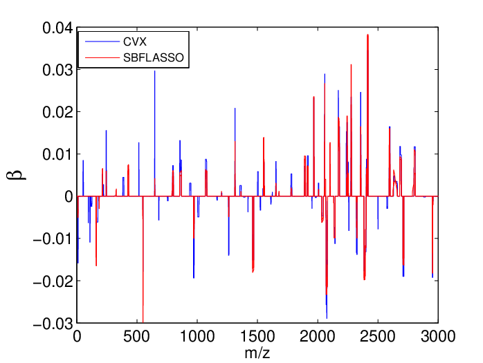
Fig 3: (a) Protein mass spectroscopy data:average profiles from normal (blue) and cancer patients (red); (b) Estimated β\beta from protein mass spectroscopy data with λ1=2,λ2=3.5\lambda_{1}=2,\lambda_{2}=3.5 by CVX (blue) and SBFLasso (red).

We apply the fused Lasso (1) to the MS data to select features (m/z sites) that can be used to predict sample labels. For each sample, the response variable is either 11 or −1-1, and the predictor variable is a vector consisting of the intensity of p=3000p=3000 sampled m/z sites. We used SBFLasso to solve the fused Lasso problem, and compared its performance to CVX and SQOPT. The results are summarized in Table 3, which shows the computational times spent by different solvers in a ten-fold cross-validation procedure for different parameters λ1\lambda_{1} and λ2\lambda_{2}. SBFLasso is consistently many times faster than CVX and SQOPT, with an approximately ten-fold speedup in almost all cases. The coefficients derived by SBFLasso and the other solvers are very similar (Figure 3b), but SBFLasso is able to achieve a sparser solution, and in addition a slightly lower objective function than CVX.

3.3 Comparative genomic hybridization (CGH) data

In tumor cells, mutations often cause a large DNA segment to be deleted or inserted in a chromosome, in a phenomena called copy number variation (CNV). Array CGH is a technique that is used to detect CNVs in a genome by labeling DNA from a test sample and normal reference sample differently using fluorophores and hybridizing to genomewide probes. The log\log ratio of the fluorescence intensity of the test DNA to the reference DNA is then calculated for each probe. A value greater than zero indicates a possible gain in DNA copies of the region around the probe, while a value less than zero suggests a possible loss. [3] demonstrated the efficiency of the fused lasso signal approximator (FLSA) for detecting CVNs using array CGH data. Next, we will show that SBFLSA is an efficient tool for solving the FLSA problem for array CGH data.

Table 4: Run times (CPU seconds) for SBFLSA on CGH data for different values of the regularization parameters λ1\lambda_{1} and λ2\lambda_{2}.
parameters SBFLSA PATHFLSA SQOPT CVX
λ1=0.10,λ2=3.0\lambda_{1}=0.10,\lambda_{2}=3.0 0.007 0.006 0.7273 0.7124
λ1=0.12,λ2=3.5\lambda_{1}=0.12,\lambda_{2}=3.5 0.007 0.005 0.6193 0.6451
λ1=0.15,λ2=3.0\lambda_{1}=0.15,\lambda_{2}=3.0 0.007 0.006 0.6161 0.6604
λ1=0.18,λ2=3.2\lambda_{1}=0.18,\lambda_{2}=3.2 0.006 0.005 0.6370 0.6244
Refer to caption
Refer to caption
Fig 4: Fused lasso applied to some GBM data. The data are shown in the left panel, and the solid red line in the right panel represents the inferred copy number β^\hat{\beta} from SBFLSA. The gray line is for y=0y=0.

We used the glioblastoma multiforme (GBM) data from [27], which contains array CGN profiling of samples from primary GBMs, a particular malignant type of brain tumor. Table 4 shows the CPU times spent by SBFLSA to solve the FLSA problem for different regularization parameters λ1\lambda_{1} and λ2\lambda_{2}. We observe that our method is significantly faster than SQOPT and CVX, with a speed improvement of about 100100 times. The performance of SBFLSA is also comparable to the path algorithm, which is specially designed, the state of the art for solving FLSA problems. Figure 4(b) plots the copy number variants detected by SBFLSA with λ1=0.10\lambda_{1}=0.10 and λ2=3.5\lambda_{2}=3.5, clearly showing the gain of DNA segments in two nearby chromosomal regions in GBM.

4 Discussion

Fused Lasso is an attractive framework for regression or classification problems with some natural ordering occurring in regression or classification coefficients. It exploits this naturally ordering by explicitly regularizing the differences between neighboring coefficients through an l1l_{1} norm regularizer. Solving the fused Lasso problem is, however, challenging because of the nondifferentiability of the objective function and the nonseparability of the variables involved in the nondifferentiable terms of the objective function. Existing solvers circumvent these difficulties by reformulating the fused Lasso problem into a smooth constrained convex optimization problem by introducing a large number of auxiliary variables and constraints, and as such, are only able to solve small or medium size fused Lasso problems.

We derived an iterative algorithm based on the split Bregman method to solve a class of fused Lasso problems, including SBFLasso for the standard fused Lasso, SBFLSA for the fused Lasso signal approximator, and SBFLSVM for fused Lasso support vector classifier, and proved their convergence properties. Preliminary experimental results for SBFLasso and SBFLSA show their efficiency for large scale problems, especially for problems with large pp, small nn, which occur in many real-world applications.

The iterative algorithm we propose is very easy to implement, involving only a few lines of code. It is also very general and can be adapted to solve a variety of fused Lasso problems with minor modifications as we have shown. In this aspect, it is very different from the path algorithm, which is specially designed for FLSA and requires significant amount of domain specific knowledge. Because of its simplicity and generality, we expect the split Bregman iterative algorithm would find its usage in a wide range of other ℓ1\ell_{1} related regularization problems.

References

  • [1] R. Tibshirani, M. Saunders, S. Rosset, J. Zhu, and K. Knight. Sparsity and smoothness via the fused lasso. J. R. Stat. Soc. Ser. B Stat. Methodol., 67(1):91–108, 2005. ISSN 1369-7412. . URL http://dx.doi.org/10.1111/j.1467-9868.2005.00490.x.
  • [2] A. Ahmed and E.P. Xing. Recovering time-varying networks of dependencies in social and biological studies. Proceedings of the National Academy of Sciences, 106(29):11878, 2009.
  • [3] R. Tibshirani and P. Wang. Spatial smoothing and hot spot detection for CGH data using the fused lasso. Biostatistics, 9:18–29, 2008.
  • [4] S. Kim, K.A. Sohn, and E.P. Xing. A multivariate regression approach to association analysis of a quantitative trait network. Bioinformatics, 25(12):i204, 2009.
  • [5] E. Philip, W. MURRAY, and A.S. Michael. User’s guide for sqopt version 7: Software for large-scale linear and quadratic programming. 2006.
  • [6] M. Grant, S. Boyd, and Y. Ye. CVX: Matlab software for disciplined convex programming. avialable at http://www. stanford. edu/boyd/cvx, 2010.
  • [7] J. Friedman, T. Hastie, H. Höfling, and R. Tibshirani. Pathwise coordinate optimization. The Annals of Applied Statistics, 1(2):302–332, 2007.
  • [8] P. Tseng. Convergence of a block coordinate descent method for nondifferentiable minimization. Journal of optimization theory and applications, 109(3):475–494, 2001.
  • [9] H. Hoefling. A path algorithm for the Fused Lasso Signal Approximator. Arxiv preprint arXiv:0910.0526, 2009.
  • [10] S. Rosset and J. Zhu. Piecewise linear regularized solution paths. Annals of Statistics, 35(3):1012, 2007.
  • [11] L. M. Brègman. A relaxation method of finding a common point of convex sets and its application to the solution of problems in convex programming. Z̆. Vyčisl. Mat. i Mat. Fiz., 7:620–631, 1967. ISSN 0044-4669.
  • [12] A. E. Çetin. Reconstruction of signals from Fourier transform samples. Signal Process., 16(2):129–148, 1989. ISSN 0165-1684. . URL http://dx.doi.org/10.1016/0165-1684(89)90092-3.
  • [13] S. Osher, M. Burger, D. Goldfarb, J. Xu, and W. Yin. An iterative regularization method for total variation-based image restoration. Multiscale Model. Simul., 4(2):460–489 (electronic), 2005. ISSN 1540-3459. . URL http://dx.doi.org/10.1137/040605412.
  • [14] T. Goldstein and S. Osher. The split Bregman method for L​1L1-regularized problems. SIAM J. Imaging Sci., 2(2):323–343, 2009. ISSN 1936-4954.
  • [15] J.-F. Cai, S. Osher, and Z. Shen. Split bregman methods and frame based image restoration. Multiscale Model. Simul., 8(2):337–369, 2009a.
  • [16] J.-F. Cai, S. Osher, and Z. Shen. Linearized Bregman iterations for compressed sensing. Math. Comp., 78(267):1515–1536, 2009b. .
  • [17] S. Osher, Y. Mao, B. Dong, and W. Yin. Fast linearized Bregman iteration for compressive sensing and sparse denoising. Communications in Mathematical Sciences, 8(2):93–111, 2010.
  • [18] W. Yin, S. Osher, D. Goldfarb, and J. Darbon. Bregman iterative algorithms for l1l_{1}-minimization with applications to compressed sensing. SIAM J. Imaging Sci., 1(1):143–168, 2008. ISSN 1936-4954.
  • [19] J.-F. Cai, E. J. Candès, and Z. Shen. A singular value thresholding algorithm for matrix completion. SIAM J. Optim., 20(4):1956–1982, 2010. ISSN 1052-6234. . URL http://dx.doi.org/10.1137/080738970.
  • [20] E.J. Candes, X. Li, Y. Ma, and J. Wright. Robust principal component analysis? Arxiv preprint arXiv:0912.3599, 2009.
  • [21] X. Zhang, M. Burger, X. Bresson, and S. Osher. Bregmanized nonlocal regularization for deconvolution and sparse reconstruction. SIAM Journal on Imaging Sciences, page to appear, 2010.
  • [22] M. R. Hestenes. Multiplier and gradient methods. J. Optimization Theory Appl., 4:303–320, 1969. ISSN 0022-3239.
  • [23] R. T. Rockafellar. A dual approach to solving nonlinear programming problems by unconstrained optimization. Math. Programming, 5:354–373, 1973. ISSN 0025-5610.
  • [24] Y. Saad. Iterative methods for sparse linear systems. Society for Industrial Mathematics, 2003.
  • [25] V. N. Vapnik. Statistical learning theory. Adaptive and Learning Systems for Signal Processing, Communications, and Control. John Wiley & Sons Inc., New York, 1998. A Wiley-Interscience Publication.
  • [26] M. Ceccarelli, A. d’Acierno, and A. Facchiano. A scale space approach for unsupervised feature selection in mass spectra classification for ovarian cancer detection. BMC Bioinformatics, 10(Suppl 12):S9, 2009. .
  • [27] M. Bredel, C. Bredel, D. Juric, G.R. Harsh, H. Vogel, L.D. Recht, and B.I. Sikic. High-resolution genome-wide mapping of genetic alterations in human glial brain tumors. Cancer research, 65(10):4088, 2005.
  • [28] J.B. Hiriart-Urruty and C. Lemaréchal. Convex Analysis and Minimization Algorithms. Springer-Verlag, Berlin, 1993.

Appendix

.1 Convergence analysis of Algorithm 1

We use some similar ideas from Cai et al. [15] to prove Theorem 1. Different from the case of Cai et al. [15], we do not require V⁡(β)V(\beta) to be differentiable, and treat the nondifferentiability of V⁡(β)V(\beta) explicitly by using its subgradient vector h∈∂V⁡(β)h\in\partial V(\beta), see the proof for details.

Proof of Theorem 1: Since all the subproblems involved in (8) are convex, the first order optimality condition of the Algorithm 1 gives

{0=hk+1+uk+LT​vk+μ1​(βk+1−ak)+μ2​LT​(L​βk+1−bk),λ1​pk+1−uk+μ1​(ak+1−βk+1)=0,λ1​qk+1−vk+μ2​(bk+1−L​βk+1)=0,uk+1=uk+δ1​(βk+1−ak+1),vk+1=vk+δ2​(L​βk+1−bk+1),\begin{cases}0=h^{k+1}+u^{k}+L^{T}v^{k}+\mu_{1}(\beta^{k+1}-a^{k})+\mu_{2}L^{T}(L\beta^{k+1}-b^{k}),\cr\lambda_{1}p^{k+1}-u^{k}+\mu_{1}(a^{k+1}-\beta^{k+1})=0,\cr\lambda_{1}q^{k+1}-v^{k}+\mu_{2}(b^{k+1}-L\beta^{k+1})=0,\cr u^{k+1}=u^{k}+\delta_{1}(\beta^{k+1}-a^{k+1}),\cr v^{k+1}=v^{k}+\delta_{2}(L\beta^{k+1}-b^{k+1}),\end{cases} (24)

where hk+1∈∂V⁡(βk+1),pk+1∈∂‖ak+1‖1h^{k+1}\in\partial V(\beta^{k+1}),p^{k+1}\in\partial\|a^{k+1}\|_{1} and qk+1∈∂‖bk+1‖1q^{k+1}\in\partial\|b^{k+1}\|_{1}.

Since β∗\beta^{*} is a solution of (2), by the first order optimality condition, there exist h∗,p∗,q∗h^{*},p^{*},q^{*} such that

h∗+λ1​p∗+λ2​LT​q∗=0h^{*}+\lambda_{1}p^{*}+\lambda_{2}L^{T}q^{*}=0 (25)

where h∗∈∂V⁡(β),p∗∈∂‖β∗‖1,q∗∈∂‖b∗‖1h^{*}\in\partial V(\beta),p^{*}\in\partial\|\beta^{*}\|_{1},q^{*}\in\partial\|b^{*}\|_{1} with b∗=L​β∗b^{*}=L\beta^{*}. Introducing new variables a∗=β∗,u∗=λ1​p∗,v∗=λ2​q∗a^{*}=\beta^{*},u^{*}=\lambda_{1}p^{*},v^{*}=\lambda_{2}q^{*}, we can formulate (25) as

{0=h∗+u∗+LT​v∗+μ1​(β∗−a∗)+μ2​LT​(L​β∗−b∗),withh∗∈∂V⁡(β)λ1​p∗−u∗+μ1​(a∗−β∗)=0,withp∗∈∂‖a∗‖1,λ1​q∗−v∗+μ2​(b∗−L​β∗)=0,withq∗∈∂‖b∗‖1,u∗=u∗+δ1​(β∗−a∗),v∗=v∗+δ2​(L​β∗−b∗).\begin{cases}0=h^{*}+u^{*}+L^{T}v^{*}+\mu_{1}(\beta^{*}-a^{*})+\mu_{2}L^{T}(L\beta^{*}-b^{*}),\quad\hbox{with}\quad h^{*}\in\partial V(\beta)\cr\lambda_{1}p^{*}-u^{*}+\mu_{1}(a^{*}-\beta^{*})=0,\quad\hbox{with}\quad p^{*}\in\partial\|a^{*}\|_{1},\cr\lambda_{1}q^{*}-v^{*}+\mu_{2}(b^{*}-L\beta^{*})=0,\quad\hbox{with}\quad q^{*}\in\partial\|b^{*}\|_{1},\cr u^{*}=u^{*}+\delta_{1}(\beta^{*}-a^{*}),\cr v^{*}=v^{*}+\delta_{2}(L\beta^{*}-b^{*}).\end{cases} (26)

Comparing (26) with (24), we can see that β∗,a∗,b∗,u∗,v∗\beta^{*},a^{*},b^{*},u^{*},v^{*} is a fix point of Algorithm 1. Denote the errors by

βek=βk−β∗,aek=ak−a∗,bek=bk−b∗,uek=uk−u∗​and​vek=vk−v∗.\beta^{k}_{e}=\beta^{k}-\beta^{*},a_{e}^{k}=a^{k}-a^{*},b_{e}^{k}=b^{k}-b^{*},u_{e}^{k}=u^{k}-u^{*}\ \hbox{and}\ v_{e}^{k}=v^{k}-v^{*}.

Subtracting the first equation of (24) by the first equation of (26), we obtain

0=hk+1−h∗+uek+LT​vek+μ1​(βek+1−aek)+μ2​LT​(L​βek+1−bek).0=h^{k+1}-h^{*}+u_{e}^{k}+L^{T}v_{e}^{k}+\mu_{1}(\beta_{e}^{k+1}-a_{e}^{k})+\mu_{2}L^{T}(L\beta_{e}^{k+1}-b_{e}^{k}).

Taking the inner product of the left and right hand sides with respect to βek+1\beta_{e}^{k+1}, we have

0\displaystyle 0 =\displaystyle= ⟨hk+1−h∗,βk+1−β∗⟩+⟨uek,βek+1⟩+⟨vek,L​βek+1⟩\displaystyle\langle h^{k+1}-h^{*},\beta^{k+1}-\beta^{*}\rangle+\langle u_{e}^{k},\beta_{e}^{k+1}\rangle+\langle v_{e}^{k},L\beta_{e}^{k+1}\rangle (27)
+μ1​‖βek+1‖22−μ1​⟨aek,βek+1⟩+μ2​‖L​βek+1‖22−μ2​⟨bek,L​βek+1⟩\displaystyle+\mu_{1}\|\beta_{e}^{k+1}\|_{2}^{2}-\mu_{1}\langle a_{e}^{k},\beta_{e}^{k+1}\rangle+\mu_{2}\|L\beta_{e}^{k+1}\|_{2}^{2}-\mu_{2}\langle b_{e}^{k},L\beta_{e}^{k+1}\rangle

Similarly, we can get

λ1​⟨pk+1−p∗,ak+1−a∗⟩+μ1​‖aek+1‖22−μ1​⟨aek+1,βek+1⟩−⟨uek,aek+1⟩=0,\lambda_{1}\langle p^{k+1}-p^{*},a^{k+1}-a^{*}\rangle+\mu_{1}\|a_{e}^{k+1}\|_{2}^{2}-\mu_{1}\langle a_{e}^{k+1},\beta_{e}^{k+1}\rangle-\langle u_{e}^{k},a_{e}^{k+1}\rangle=0, (28)
λ2​⟨qk+1−q∗,bk+1−b∗⟩+μ2​‖bek+1‖22−μ2​⟨bek+1,L​βek+1⟩−⟨vek,bek+1⟩=0.\lambda_{2}\langle q^{k+1}-q^{*},b^{k+1}-b^{*}\rangle+\mu_{2}\|b_{e}^{k+1}\|_{2}^{2}-\mu_{2}\langle b_{e}^{k+1},L\beta_{e}^{k+1}\rangle-\langle v_{e}^{k},b_{e}^{k+1}\rangle=0. (29)

Summing (27), (28) and (29) together, we get

⟨hk+1−h∗,βk+1−β∗⟩+λ1​⟨pk+1−p∗,ak+1−a∗⟩+λ2​⟨qk+1−q∗,bk+1−b∗⟩\displaystyle\langle h^{k+1}-h^{*},\beta^{k+1}-\beta^{*}\rangle+\lambda_{1}\langle p^{k+1}-p^{*},a^{k+1}-a^{*}\rangle+\lambda_{2}\langle q^{k+1}-q^{*},b^{k+1}-b^{*}\rangle
+μ1​(‖βek+1‖22+‖aek+1‖22−⟨βek+1,aek+aek+1⟩)+μ2​(‖L​βek+1‖22+‖bek+1‖22CLOSE\displaystyle+\mu_{1}(\|\beta_{e}^{k+1}\|_{2}^{2}+\|a_{e}^{k+1}\|_{2}^{2}-\langle\beta_{e}^{k+1},a_{e}^{k}+a_{e}^{k+1}\rangle)+\mu_{2}(\|L\beta_{e}^{k+1}\|_{2}^{2}+\|b_{e}^{k+1}\|_{2}^{2}
OPEN−⟨L​βek+1,bek+bek+1⟩)+⟨uek,βek+1−aek+1⟩+⟨vek,L​βek+1−bek+1⟩=0\displaystyle-\langle L\beta_{e}^{k+1},b_{e}^{k}+b_{e}^{k+1}\rangle)+\langle u_{e}^{k},\beta_{e}^{k+1}-a_{e}^{k+1}\rangle+\langle v_{e}^{k},L\beta_{e}^{k+1}-b_{e}^{k+1}\rangle=0 (30)

Furthermore, by subtracting the fourth equation of (24) by the one of (26), we have

uek+1=uek+δ1​(βek+1−aek+1).u_{e}^{k+1}=u_{e}^{k}+\delta_{1}(\beta_{e}^{k+1}-a_{e}^{k+1}).

Taking square of both sides of the above equation implies

⟨uek,βek+1−aek+1⟩=12​δ1​(‖uek+1‖22−‖uek‖22)−δ12​‖βek+1−aek+1‖22.\langle u_{e}^{k},\beta_{e}^{k+1}-a_{e}^{k+1}\rangle=\frac{1}{2\delta_{1}}(\|u_{e}^{k+1}\|_{2}^{2}-\|u_{e}^{k}\|_{2}^{2})-\frac{\delta_{1}}{2}\|\beta_{e}^{k+1}-a_{e}^{k+1}\|_{2}^{2}. (31)

Similarly, we have

⟨vek,L​βek+1−bek+1⟩=12​δ2​(‖vek+1‖22−‖vek‖22)−δ22​‖L​βek+1−bek+1‖22.\langle v_{e}^{k},L\beta_{e}^{k+1}-b_{e}^{k+1}\rangle=\frac{1}{2\delta_{2}}(\|v_{e}^{k+1}\|_{2}^{2}-\|v_{e}^{k}\|_{2}^{2})-\frac{\delta_{2}}{2}\|L\beta_{e}^{k+1}-b_{e}^{k+1}\|_{2}^{2}. (32)

Substituting (31) and (32) into (30) yields

12​δ1​(‖uek‖22−‖uek+1‖22)+12​δ2​(‖vek‖22−‖vek+1‖22)\displaystyle\frac{1}{2\delta_{1}}(\|u_{e}^{k}\|_{2}^{2}-\|u_{e}^{k+1}\|_{2}^{2})+\frac{1}{2\delta_{2}}(\|v_{e}^{k}\|_{2}^{2}-\|v_{e}^{k+1}\|_{2}^{2})
=\displaystyle= ⟨hk+1−h∗,βk+1−β∗⟩+λ1​⟨pk+1−p∗,ak+1−a∗⟩+λ2​⟨qk+1−q∗,bk+1−b∗⟩\displaystyle\langle h^{k+1}-h^{*},\beta^{k+1}-\beta^{*}\rangle+\lambda_{1}\langle p^{k+1}-p^{*},a^{k+1}-a^{*}\rangle+\lambda_{2}\langle q^{k+1}-q^{*},b^{k+1}-b^{*}\rangle
+μ1​(‖βek+1‖22+‖aek+1‖22−⟨βek+1,aek+aek+1⟩−δ12​μ1​‖βek+1−aek+1‖22)\displaystyle+\mu_{1}(\|\beta_{e}^{k+1}\|_{2}^{2}+\|a_{e}^{k+1}\|_{2}^{2}-\langle\beta_{e}^{k+1},a_{e}^{k}+a_{e}^{k+1}\rangle-\frac{\delta_{1}}{2\mu_{1}}\|\beta_{e}^{k+1}-a_{e}^{k+1}\|_{2}^{2})
+μ2​(‖L​βek+1‖22+‖bek+1‖22−⟨L​βek+1,bek+bek+1⟩−δ22​μ2​‖L​βek+1−bek+1‖22)+\mu_{2}(\|L\beta_{e}^{k+1}\|_{2}^{2}+\|b_{e}^{k+1}\|_{2}^{2}-\langle L\beta_{e}^{k+1},b_{e}^{k}+b_{e}^{k+1}\rangle-\frac{\delta_{2}}{2\mu_{2}}\|L\beta_{e}^{k+1}-b_{e}^{k+1}\|_{2}^{2}) (33)

Note that for any 𝐱,𝐲,𝐳∈ℝp\mathbf{x},\mathbf{y},\mathbf{z}\in\mathbb{R}^{p}, we have

‖𝐱‖22±⟨𝐱,𝐲+𝐳⟩+‖𝐲‖22=12​‖𝐱±𝐲‖22+12​‖𝐱±𝐳‖22+12​(‖𝐲‖22−‖𝐳‖22).\|\mathbf{x}\|_{2}^{2}\pm\langle\mathbf{x},\mathbf{y}+\mathbf{z}\rangle+\|\mathbf{y}\|_{2}^{2}=\frac{1}{2}\|\mathbf{x}\pm\mathbf{y}\|_{2}^{2}+\frac{1}{2}\|\mathbf{x}\pm\mathbf{z}\|_{2}^{2}+\frac{1}{2}(\|\mathbf{y}\|_{2}^{2}-\|\mathbf{z}\|_{2}^{2}). (34)

Using this elementary equation, (33) can be transformed to

12​δ1​(‖uek‖22−‖uek+1‖22)+12​δ2​(‖vek‖22−‖vek+1‖22)\displaystyle\frac{1}{2\delta_{1}}(\|u_{e}^{k}\|_{2}^{2}-\|u_{e}^{k+1}\|_{2}^{2})+\frac{1}{2\delta_{2}}(\|v_{e}^{k}\|_{2}^{2}-\|v_{e}^{k+1}\|_{2}^{2})
=\displaystyle= ⟨hk+1−h∗,βk+1−β∗⟩+λ1​⟨pk+1−p∗,ak+1−a∗⟩+λ2​⟨qk+1−q∗,bk+1−b∗⟩\displaystyle\langle h^{k+1}-h^{*},\beta^{k+1}-\beta^{*}\rangle+\lambda_{1}\langle p^{k+1}-p^{*},a^{k+1}-a^{*}\rangle+\lambda_{2}\langle q^{k+1}-q^{*},b^{k+1}-b^{*}\rangle
+μ12​(‖βek+1−aek‖22+‖aek+1‖22−‖aek‖22+μ1−δ1μ1​‖βek+1−aek+1‖22)\displaystyle+\frac{\mu_{1}}{2}\left(\|\beta_{e}^{k+1}-a_{e}^{k}\|_{2}^{2}+\|a_{e}^{k+1}\|_{2}^{2}-\|a_{e}^{k}\|_{2}^{2}+\frac{\mu_{1}-\delta_{1}}{\mu_{1}}\|\beta_{e}^{k+1}-a_{e}^{k+1}\|_{2}^{2}\right)
+μ22​(‖L​βek+1−bek‖22+‖bek+1‖22−‖bek‖22+μ2−δ2μ2​‖L​βek+1−bek+1‖22)\displaystyle+\frac{\mu_{2}}{2}\left(\|L\beta_{e}^{k+1}-b_{e}^{k}\|_{2}^{2}+\|b_{e}^{k+1}\|_{2}^{2}-\|b_{e}^{k}\|_{2}^{2}+\frac{\mu_{2}-\delta_{2}}{\mu_{2}}\|L\beta_{e}^{k+1}-b_{e}^{k+1}\|_{2}^{2}\right)

Summing the above equation from k=0k=0 to k=Kk=K yields

12​δ1​(‖ue0‖22−‖ueK+1‖22)+12​δ2​(‖ve0‖22−‖veK+1‖22)\displaystyle\frac{1}{2\delta_{1}}(\|u_{e}^{0}\|_{2}^{2}-\|u_{e}^{K+1}\|_{2}^{2})+\frac{1}{2\delta_{2}}(\|v_{e}^{0}\|_{2}^{2}-\|v_{e}^{K+1}\|_{2}^{2}) (35)
+μ12​(‖ae0‖22−‖aeK+1‖22)+μ22​(‖be0‖22−‖beK+1‖22)\displaystyle+\frac{\mu_{1}}{2}(\|a_{e}^{0}\|_{2}^{2}-\|a_{e}^{K+1}\|_{2}^{2})+\frac{\mu_{2}}{2}(\|b_{e}^{0}\|_{2}^{2}-\|b_{e}^{K+1}\|_{2}^{2})
=\displaystyle= ∑k=0K⟨hk+1−h∗,βk+1−β∗⟩+λ1​∑k=0K⟨pk+1−p∗,ak+1−a∗⟩\displaystyle\sum_{k=0}^{K}\langle h^{k+1}-h^{*},\beta^{k+1}-\beta^{*}\rangle+\lambda_{1}\sum_{k=0}^{K}\langle p^{k+1}-p^{*},a^{k+1}-a^{*}\rangle
+λ2∑k=0K⟨qk+1−q∗,bk+1−b∗⟩+μ12∑k=0K∥βek+1−aek∥22+μ1−δ1μ1∑k=0K∥βek+1−aek+1∥22\displaystyle+\lambda_{2}\sum_{k=0}^{K}\langle q^{k+1}-q^{*},b^{k+1}-b^{*}\rangle+\frac{\mu_{1}}{2}\sum_{k=0}^{K}\|\beta_{e}^{k+1}-a_{e}^{k}\|_{2}^{2}+\frac{\mu_{1}-\delta_{1}}{\mu_{1}}\sum_{k=0}^{K}\|\beta_{e}^{k+1}-a_{e}^{k+1}\|_{2}^{2}
+μ22∑k=0K∥Lβek+1−bek∥22+μ2−δ2μ2∑k=0K∥Lβek+1−bek+1∥22\displaystyle+\frac{\mu_{2}}{2}\sum_{k=0}^{K}\|L\beta_{e}^{k+1}-b_{e}^{k}\|_{2}^{2}+\frac{\mu_{2}-\delta_{2}}{\mu_{2}}\sum_{k=0}^{K}\|L\beta_{e}^{k+1}-b_{e}^{k+1}\|_{2}^{2}

The fact that hk+1∈∂V⁡(βk+1),h∗∈∂V⁡(β∗)h^{k+1}\in\partial V(\beta^{k+1}),h^{*}\in\partial V(\beta^{*}) and V⁡(β)V(\beta) is convex implies

⟨hk+1−h∗,βk+1−β∗⟩\displaystyle\langle h^{k+1}-h^{*},\beta^{k+1}-\beta^{*}\rangle (36)
=\displaystyle= V⁡(βk+1)−V⁡(β∗)−⟨h∗,βk+1−β∗⟩+V⁡(β∗)−V⁡(βk+1)−⟨hk+1,βk+1−β∗⟩\displaystyle V(\beta^{k+1})-V(\beta^{*})-\langle h^{*},\beta^{k+1}-\beta^{*}\rangle+V(\beta^{*})-V(\beta^{k+1})-\langle h^{k+1},\beta^{k+1}-\beta^{*}\rangle
≥\displaystyle\geq 0\displaystyle 0

by the definition of subgradient. Similarly, ⟨pk+1−p∗,ak+1−a∗⟩≥0,⟨qk+1−q∗,bk+1−b∗⟩≥0\langle p^{k+1}-p^{*},a^{k+1}-a^{*}\rangle\geq 0,\langle q^{k+1}-q^{*},b^{k+1}-b^{*}\rangle\geq 0. Together with the fact that 0<δ1≤μ10<\delta_{1}\leq\mu_{1} and 0<δ2≤μ20<\delta_{2}\leq\mu_{2}, all terms involved in (35) are nonnegative. Therefore,

∑k=0∞⟨hk+1−h∗,βk+1−β∗⟩≤12​δ1​‖ue0‖22+12​δ2​‖ve0‖22+μ12​‖ae0‖22+μ22​‖be0‖22\sum_{k=0}^{\infty}\langle h^{k+1}-h^{*},\beta^{k+1}-\beta^{*}\rangle\leq\frac{1}{2\delta_{1}}\|u_{e}^{0}\|_{2}^{2}+\frac{1}{2\delta_{2}}\|v_{e}^{0}\|_{2}^{2}+\frac{\mu_{1}}{2}\|a_{e}^{0}\|_{2}^{2}+\frac{\mu_{2}}{2}\|b_{e}^{0}\|_{2}^{2}

which leads to

limk→∞⟨hk−h∗,βk−β∗⟩=0.\lim_{k\rightarrow\infty}\langle h^{k}-h^{*},\beta^{k}-\beta^{*}\rangle=0.

Together with (36) leads to

limk→∞V⁡(βk)−V⁡(β∗)−⟨h∗,βk−β∗⟩=0.\lim_{k\rightarrow\infty}V(\beta^{k})-V(\beta^{*})-\langle h^{*},\beta^{k}-\beta^{*}\rangle=0. (37)

Similarly, we can prove

λ1​limk→∞‖ak‖1−‖a∗‖1−⟨ak−a∗,p∗⟩=0,\lambda_{1}\lim_{k\rightarrow\infty}\|a^{k}\|_{1}-\|a^{*}\|_{1}-\langle a^{k}-a^{*},p^{*}\rangle=0, (38)
λ2​limk→∞‖bk‖1−‖b∗‖1−⟨bk−b∗,q∗⟩=0,\lambda_{2}\lim_{k\rightarrow\infty}\|b^{k}\|_{1}-\|b^{*}\|_{1}-\langle b^{k}-b^{*},q^{*}\rangle=0, (39)
limk→∞‖βk−ak‖2=0andlimk→∞‖L​βk−bk‖2=0.\lim_{k\rightarrow\infty}\|\beta^{k}-a^{k}\|_{2}=0\quad\hbox{and}\quad\lim_{k\rightarrow\infty}\|L\beta^{k}-b^{k}\|_{2}=0. (40)

Since ∥⋅∥1\|\cdot\|_{1} is continuous, by (38),(39) and (40), we obtain

λ1​limk→∞‖βk‖1−‖β∗‖1−⟨βk−β∗,p∗⟩=0,\lambda_{1}\lim_{k\rightarrow\infty}\|\beta^{k}\|_{1}-\|\beta^{*}\|_{1}-\langle\beta^{k}-\beta^{*},p^{*}\rangle=0, (41)
λ2​limk→∞‖L​βk‖1−‖L​β∗‖1−⟨L​βk−L​β∗,q∗⟩=0.\lambda_{2}\lim_{k\rightarrow\infty}\|L\beta^{k}\|_{1}-\|L\beta^{*}\|_{1}-\langle L\beta^{k}-L\beta^{*},q^{*}\rangle=0. (42)

Summing (37),(41) and (42) yields

limk→∞V⁡(βk)+λ1​‖βk‖1+λ2​‖L​βk‖1−(V⁡(β∗)+λ1​‖β∗‖1+λ2​‖L​β∗‖1)\displaystyle\lim_{k\rightarrow\infty}V(\beta^{k})+\lambda_{1}\|\beta^{k}\|_{1}+\lambda_{2}\|L\beta^{k}\|_{1}-(V(\beta^{*})+\lambda_{1}\|\beta^{*}\|_{1}+\lambda_{2}\|L\beta^{*}\|_{1})
+⟨βk−β∗,h∗+p∗+LT​q∗⟩=0\displaystyle\qquad+\langle\beta^{k}-\beta^{*},h^{*}+p^{*}+L^{T}q^{*}\rangle=0

This together with (25) proves

limk→∞V⁡(βk)+λ1​‖βk‖1+λ2​‖L​βk‖1=V⁡(β∗)+λ1​‖β∗‖1+λ2​‖L​β∗‖1.\lim_{k\rightarrow\infty}V(\beta^{k})+\lambda_{1}\|\beta^{k}\|_{1}+\lambda_{2}\|L\beta^{k}\|_{1}=V(\beta^{*})+\lambda_{1}\|\beta^{*}\|_{1}+\lambda_{2}\|L\beta^{*}\|_{1}. (43)

Next, we prove that

limk→∞‖βk−β∗‖2=0\lim_{k\rightarrow\infty}\|\beta^{k}-\beta^{*}\|_{2}=0 (44)

whenever (2) has a unique solution.

It is proved by contradiction. Let Φ⁡(β)=V⁡(β)+λ1​‖β‖1+λ2​‖L​β‖1\Phi(\beta)=V(\beta)+\lambda_{1}\|\beta\|_{1}+\lambda_{2}\|L\beta\|_{1}. Then Φ⁡(β)\Phi(\beta) is a convex, lower continuous function. Since β∗\beta^{*} is the unique minimizer, we have Φ⁡(β)>Φ⁡(β∗)\Phi(\beta)>\Phi(\beta^{*}) for all β≠β∗\beta\neq\beta^{*}. If (44) does not hold, there exists a subsequence βki\beta^{k_{i}} such that ‖βki−β∗‖>ϵ\|\beta^{k_{i}}-\beta^{*}\|>\epsilon for some ϵ>0\epsilon>0 and for all ii. Then Φ⁡(βki)>min⁡{Φ⁡(β):‖β−β∗‖2=ϵ}\Phi(\beta^{k_{i}})>\min\{\Phi(\beta):\|\beta-\beta^{*}\|_{2}=\epsilon\}. Indeed, let γ\gamma be the intersection of the sphere {β:‖β−β∗‖2=ϵ}\{\beta:\|\beta-\beta^{*}\|_{2}=\epsilon\} and line segment from β∗\beta^{*} to βki\beta^{k_{i}}, then there exists a positive number t∈(0,1)t\in(0,1) such that γ=t​β∗+(1−t)​βki\gamma=t\beta^{*}+(1-t)\beta^{k_{i}}. By the convexity of Φ\Phi and the definition of β∗\beta^{*}, we have

Φ⁡(βki)\displaystyle\Phi(\beta^{k_{i}}) >\displaystyle> t​Φ​(β∗)+(1−t)​Φ​(βki)≥Φ⁡(t​β∗+(1−t)​βki)\displaystyle t\Phi(\beta^{*})+(1-t)\Phi(\beta^{k_{i}})\geq\Phi(t\beta^{*}+(1-t)\beta^{k_{i}})
=\displaystyle= Φ⁡(γ)≥min⁡{Φ⁡(β):‖β−β∗‖2=ϵ}.\displaystyle\Phi(\gamma)\geq\min\{\Phi(\beta):\|\beta-\beta^{*}\|_{2}=\epsilon\}.

Denote β~=arg⁡min⁡{Φ⁡(β):‖β−β∗‖2=ϵ}\tilde{\beta}=\arg\min\{\Phi(\beta):\|\beta-\beta^{*}\|_{2}=\epsilon\} . By applying (43), we have

Φ⁡(β∗)=limi→∞​∞Φ⁡(βki)≥Φ⁡(β~)>Φ⁡(β∗),\Phi(\beta^{*})=\lim_{i\rightarrow\infty\infty}\Phi(\beta^{k_{i}})\geq\Phi(\tilde{\beta})>\Phi(\beta^{*}),

which is a contradiction.       

.2 Convergence analysis of Algorithm 2

Now we give the proof of Theorem 2. The main idea is the same as the one in [15]. However, due to the extra bias term β0\beta_{0} and the hinge loss, the terms involved in our proof are more complicated.

Since all the subproblems involved in (18) are convex, the first order optimality condition gives

{(μ1​I+μ2​LT​L+μ3​XT​Y2​Xμ3​XT​Y​yμ3​yT​Y​Xμ3​yT​y)​(βk+1β0k+1)=μ1​(ak−μ1−1​uk0)+μ2​(LT0)​(bk−μ2−1​vk)+μ3​(XT​YyT)​(𝟏−ck+μ3−1​wk)λ1​pk+1−uk+μ1​(ak+1−βk+1)=0,λ2​qk+1−vk+μ2​(bk+1−L​βk+1)=0,1n​sk+1−wk+μ3​(ck+1+Y​X​βk+1+β0k+1​y−𝟏)=0,uk+1=uk+δ1​(βk+1−ak+1),vk+1=vk+δ2​(L​βk+1−bk+1),wk+1=wk+δ3​(𝟏−Y​X​βk+1−β0k+1​y−ck+1),\begin{cases}\left(\begin{matrix}\mu_{1}I+\mu_{2}L^{T}L+\mu_{3}X^{T}Y^{2}X&\mu_{3}X^{T}Yy\cr\mu_{3}y^{T}YX&\mu_{3}y^{T}y\end{matrix}\right)\left(\begin{matrix}\beta^{k+1}\cr\beta_{0}^{k+1}\end{matrix}\right)\cr=\mu_{1}\left(\begin{matrix}a^{k}-\mu_{1}^{-1}u^{k}\cr 0\end{matrix}\right)+\mu_{2}\left(\begin{matrix}L^{T}\cr 0\end{matrix}\right)(b^{k}-\mu_{2}^{-1}v^{k})+\mu_{3}\left(\begin{matrix}X^{T}Y\cr y^{T}\end{matrix}\right)(\mathbf{1}-c^{k}+\mu_{3}^{-1}w^{k})\cr\lambda_{1}p^{k+1}-u^{k}+\mu_{1}(a^{k+1}-\beta^{k+1})=0,\cr\lambda_{2}q^{k+1}-v^{k}+\mu_{2}(b^{k+1}-L\beta^{k+1})=0,\cr\frac{1}{n}s^{k+1}-w^{k}+\mu_{3}(c^{k+1}+YX\beta^{k+1}+\beta_{0}^{k+1}y-\mathbf{1})=0,\cr u^{k+1}=u^{k}+\delta_{1}(\beta^{k+1}-a^{k+1}),\cr v^{k+1}=v^{k}+\delta_{2}(L\beta^{k+1}-b^{k+1}),\cr w^{k+1}=w^{k}+\delta_{3}(\mathbf{1}-YX\beta^{k+1}-\beta_{0}^{k+1}y-c^{k+1}),\end{cases} (45)

where pk+1∈∂‖ak+1‖1,qk+1∈∂‖bk+1‖1p^{k+1}\in\partial\|a^{k+1}\|_{1},q^{k+1}\in\partial\|b^{k+1}\|_{1} and sk+1∈∂‖ck+1‖1s^{k+1}\in\partial\|c^{k+1}\|_{1}. This simple observation will be used in our proof for the convergence of SBFLSVM.

Proof of Theorem 2. Let (β∗,β0∗)(\beta^{*},\beta_{0}^{*}) be an arbitrary minimizer of (16). By the first order optimality condition, there exist p∗,q∗p^{*},q^{*} and s∗s^{*} such that

{−1n​XT​Y​s∗+λ1​p∗+λ2​LT​q∗=0,yT​s∗=0,\begin{cases}-\frac{1}{n}X^{T}Ys^{*}+\lambda_{1}p^{*}+\lambda_{2}L^{T}q^{*}=0,\cr y^{T}s^{*}=0,\end{cases} (46)

where si∗∈∂(ci∗)+s_{i}^{*}\in\partial(c_{i}^{*})_{+} with ci∗=1−yi(𝐱iTβ∗+β0∗),i=1,…,n,p∗∈∂∥β∗∥1c_{i}^{*}=1-y_{i}(\mathbf{x}_{i}^{T}\beta^{*}+\beta_{0}^{*}),i=1,\ldots,n,p^{*}\in\partial\|\beta^{*}\|_{1}, q∗∈∂‖b∗‖1q^{*}\in\partial\|b^{*}\|_{1} with b∗=L​β∗b^{*}=L\beta^{*}. Introducing new variables a∗=β∗,u∗=λ1​p∗,v∗=λ2​q∗a^{*}=\beta^{*},u^{*}=\lambda_{1}p^{*},v^{*}=\lambda_{2}q^{*} and w∗=1n​s∗w^{*}=\frac{1}{n}s^{*}, we can formulate (46) as

{(μ1​I+μ2​LT​L+μ3​XT​Y2​Xμ3​XT​Y​yμ3​yT​Y​Xμ3​yT​y)​(β∗β0∗)=μ1​(a∗−μ1−1​u∗0)+μ2​(LT0)​(b∗−μ2−1​v∗)+μ3​(XT​YyT)​(𝟏−c∗+μ3−1​w∗)λ1​p∗−u∗+μ1​(a∗−β∗)=0,withp∗∈∂‖a∗‖1λ2​q∗−v∗+μ2​(b∗−L​β∗)=0,withq∗∈∂‖b∗‖11n​s∗−w∗+μ3​(c∗+Y​X​β∗+β0∗​y−𝟏)=0,withs∗∈∂(∑i=1n(ci)+)u∗=u∗+δ1​(β∗−a∗),v∗=v∗+δ2​(L​β∗−b∗),w∗=w∗+δ3​(𝟏−Y​X​β∗−β0∗​y−c∗).\begin{cases}\left(\begin{matrix}\mu_{1}I+\mu_{2}L^{T}L+\mu_{3}X^{T}Y^{2}X&\mu_{3}X^{T}Yy\cr\mu_{3}y^{T}YX&\mu_{3}y^{T}y\end{matrix}\right)\left(\begin{matrix}\beta^{*}\cr\beta_{0}^{*}\end{matrix}\right)\cr=\mu_{1}\left(\begin{matrix}a^{*}-\mu_{1}^{-1}u^{*}\cr 0\end{matrix}\right)+\mu_{2}\left(\begin{matrix}L^{T}\cr 0\end{matrix}\right)(b^{*}-\mu_{2}^{-1}v^{*})+\mu_{3}\left(\begin{matrix}X^{T}Y\cr y^{T}\end{matrix}\right)(\mathbf{1}-c^{*}+\mu_{3}^{-1}w^{*})\cr\lambda_{1}p^{*}-u^{*}+\mu_{1}(a^{*}-\beta^{*})=0,\quad\hbox{with}\quad p^{*}\in\partial\|a^{*}\|_{1}\cr\lambda_{2}q^{*}-v^{*}+\mu_{2}(b^{*}-L\beta^{*})=0,\quad\hbox{with}\quad q^{*}\in\partial\|b^{*}\|_{1}\cr\frac{1}{n}s^{*}-w^{*}+\mu_{3}(c^{*}+YX\beta^{*}+\beta_{0}^{*}y-\mathbf{1})=0,\quad\hbox{with}\quad s^{*}\in\partial(\sum_{i=1}^{n}(c_{i})_{+})\cr u^{*}=u^{*}+\delta_{1}(\beta^{*}-a^{*}),\cr v^{*}=v^{*}+\delta_{2}(L\beta^{*}-b^{*}),\cr w^{*}=w^{*}+\delta_{3}(\mathbf{1}-YX\beta^{*}-\beta_{0}^{*}y-c^{*}).\cr\end{cases} (47)

Therefore, β∗,β0∗,a∗,b∗,c∗,u∗,v∗,w∗\beta^{*},\beta_{0}^{*},a^{*},b^{*},c^{*},u^{*},v^{*},w^{*} is a fixed point of (45). Denote the errors by

βek=βk−β∗,β0​ek=β0k−β0∗,aek=ak−a∗,bek=bk−b∗,\beta_{e}^{k}=\beta^{k}-\beta^{*},\beta_{0e}^{k}=\beta_{0}^{k}-\beta_{0}^{*},a_{e}^{k}=a^{k}-a^{*},b_{e}^{k}=b^{k}-b^{*},
cek=ck−c∗,uek=uk−u∗,vek=vk−v∗​and​wek=wk−w∗c_{e}^{k}=c^{k}-c^{*},u_{e}^{k}=u^{k}-u^{*},v_{e}^{k}=v^{k}-v^{*}\ \hbox{and}\ w_{e}^{k}=w^{k}-w^{*}

Subtracting the first equation of (45) by the first equation of (47), we obtain

(μ1​I+μ2​LT​L+μ3​XT​Y2​Xμ3​XT​Y​yμ3​yT​Y​Xμ3​yT​y)​(βek+1β0​ek+1)\displaystyle\left(\begin{matrix}\mu_{1}I+\mu_{2}L^{T}L+\mu_{3}X^{T}Y^{2}X&\mu_{3}X^{T}Yy\cr\mu_{3}y^{T}YX&\mu_{3}y^{T}y\end{matrix}\right)\left(\begin{matrix}\beta_{e}^{k+1}\cr\beta_{0e}^{k+1}\end{matrix}\right)
=μ1​(aek−μ1−1​uek0)+μ2​(LT0)​(bek−μ2−1​vek)+μ3​(XT​YyT)​(−cek+μ3−1​wek)\displaystyle=\mu_{1}\left(\begin{matrix}a_{e}^{k}-\mu_{1}^{-1}u_{e}^{k}\cr 0\end{matrix}\right)+\mu_{2}\left(\begin{matrix}L^{T}\cr 0\end{matrix}\right)(b_{e}^{k}-\mu_{2}^{-1}v_{e}^{k})+\mu_{3}\left(\begin{matrix}X^{T}Y\cr y^{T}\end{matrix}\right)(-c_{e}^{k}+\mu_{3}^{-1}w_{e}^{k})

Taking the inner product of the left and right hand sides with respect to ((βek+1)T,β0​ek+1)T,((\beta_{e}^{k+1})^{T},\beta_{0e}^{k+1})^{T}, we have

⟨(μ1​I+μ2​LT​L+μ3​XT​Y2​X)​βek+1+μ3​XT​Y​y​β0​ek+1,βek+1⟩+μ3​⟨Y​X​βek+1+y​β0​ek+1,y​β0​ek+1⟩\displaystyle\langle(\mu_{1}I+\mu_{2}L^{T}L+\mu_{3}X^{T}Y^{2}X)\beta_{e}^{k+1}+\mu_{3}X^{T}Yy\beta_{0e}^{k+1},\beta_{e}^{k+1}\rangle+\mu_{3}\langle YX\beta_{e}^{k+1}+y\beta_{0e}^{k+1},y\beta_{0e}^{k+1}\rangle (48)
=\displaystyle= μ1​⟨aek,βek+1⟩−⟨uek,βek+1⟩+μ2​⟨bek,L​βek+1⟩−⟨vek,L​βek+1⟩\displaystyle\mu_{1}\langle a_{e}^{k},\beta_{e}^{k+1}\rangle-\langle u_{e}^{k},\beta_{e}^{k+1}\rangle+\mu_{2}\langle b_{e}^{k},L\beta_{e}^{k+1}\rangle-\langle v_{e}^{k},L\beta_{e}^{k+1}\rangle
−μ3​⟨cek,Y​X​βek+1⟩+⟨wek,Y​X​βek+1⟩−μ3​⟨cek,y​β0​ek+1⟩+⟨wek,y​β0​ek+1⟩.\displaystyle-\mu_{3}\langle c_{e}^{k},YX\beta_{e}^{k+1}\rangle+\langle w_{e}^{k},YX\beta_{e}^{k+1}\rangle-\mu_{3}\langle c_{e}^{k},y\beta_{0e}^{k+1}\rangle+\langle w_{e}^{k},y\beta_{0e}^{k+1}\rangle.

The same manipulations applied to the second (third, fourth) of equation (45) and the second (third, fourth) of equation (47) lead to

λ1​⟨pk+1−p∗,ak+1−a∗⟩+μ1​‖aek+1‖22−⟨uek,aek+1⟩−μ1​⟨βek+1,aek+1⟩=0.\lambda_{1}\langle p^{k+1}-p^{*},a^{k+1}-a^{*}\rangle+\mu_{1}\|a_{e}^{k+1}\|^{2}_{2}-\langle u_{e}^{k},a_{e}^{k+1}\rangle-\mu_{1}\langle\beta_{e}^{k+1},a_{e}^{k+1}\rangle=0. (49)
λ2​⟨qk+1−q∗,bk+1−b∗⟩+μ2​‖bek+1‖22−⟨vek,bek+1⟩−μ2​⟨L​βek+1,bek+1⟩=0.\lambda_{2}\langle q^{k+1}-q^{*},b^{k+1}-b^{*}\rangle+\mu_{2}\|b_{e}^{k+1}\|_{2}^{2}-\langle v_{e}^{k},b_{e}^{k+1}\rangle-\mu_{2}\langle L\beta_{e}^{k+1},b_{e}^{k+1}\rangle=0. (50)
1n​⟨sk+1−s∗,ck+1−c∗⟩+μ3​‖cek+1‖22−⟨wek,cek+1⟩+μ3​⟨Y​X​βek+1+β0​ek+1​y,cek+1⟩=0.\frac{1}{n}\langle s^{k+1}-s^{*},c^{k+1}-c^{*}\rangle+\mu_{3}\|c_{e}^{k+1}\|_{2}^{2}-\langle w_{e}^{k},c_{e}^{k+1}\rangle+\mu_{3}\langle YX\beta_{e}^{k+1}+\beta_{0e}^{k+1}y,c_{e}^{k+1}\rangle=0. (51)

By summing equations (48), (49), (50) and (51), we get

λ1​⟨pk+1−p∗,ak+1−a∗⟩+λ2​⟨qk+1−q∗,bk+1−b∗⟩+1n​⟨sk+1−s∗,ck+1−c∗⟩\displaystyle\quad\lambda_{1}\langle p^{k+1}-p^{*},a^{k+1}-a^{*}\rangle+\lambda_{2}\langle q^{k+1}-q^{*},b^{k+1}-b^{*}\rangle+\frac{1}{n}\langle s^{k+1}-s^{*},c^{k+1}-c^{*}\rangle
+μ1​(‖βek+1‖22−⟨βek+1,aek+1+aek⟩+‖aek+1‖22)\displaystyle+\mu_{1}(\|\beta_{e}^{k+1}\|_{2}^{2}-\langle\beta_{e}^{k+1},a_{e}^{k+1}+a_{e}^{k}\rangle+\|a_{e}^{k+1}\|_{2}^{2})
+μ2​(‖L​βek+1‖22−⟨bek+1+bek,L​βek+1⟩+‖bek+1‖22)\displaystyle+\mu_{2}(\|L\beta_{e}^{k+1}\|_{2}^{2}-\langle b_{e}^{k+1}+b_{e}^{k},L\beta_{e}^{k+1}\rangle+\|b_{e}^{k+1}\|_{2}^{2})
+μ3​(‖Y​X​βek+1+y​β0​ek+1‖22+μ3​⟨Y​X​βek+1+y​β0​ek+1,cek+1+cek⟩+‖cek+1‖22)\displaystyle+\mu_{3}(\|YX\beta_{e}^{k+1}+y\beta_{0e}^{k+1}\|_{2}^{2}+\mu_{3}\langle YX\beta_{e}^{k+1}+y\beta_{0e}^{k+1},c_{e}^{k+1}+c_{e}^{k}\rangle+\|c_{e}^{k+1}\|_{2}^{2})
+⟨uek,βek+1−aek+1⟩+⟨vek,L​βek+1−bek+1⟩−⟨wek,Y​X​βek+1+y​β0​ek+1+cek+1⟩=0.\displaystyle+\langle u_{e}^{k},\beta_{e}^{k+1}-a_{e}^{k+1}\rangle+\langle v_{e}^{k},L\beta_{e}^{k+1}-b_{e}^{k+1}\rangle-\langle w_{e}^{k},YX\beta_{e}^{k+1}+y\beta_{0e}^{k+1}+c_{e}^{k+1}\rangle=0.
(52)

Furthermore, subtracting the fifth equation of (45) by the fifth equation of (47), we have

uek+1=uek+δ1​(βek+1−aek+1).u_{e}^{k+1}=u_{e}^{k}+\delta_{1}(\beta_{e}^{k+1}-a_{e}^{k+1}).

which leads to

⟨uek,βek+1−aek+1⟩=12​δ1​(‖uek+1‖22−‖uek‖22)−δ12​‖βek+1−aek+1‖22.\langle u_{e}^{k},\beta_{e}^{k+1}-a_{e}^{k+1}\rangle=\frac{1}{2\delta_{1}}(\|u_{e}^{k+1}\|_{2}^{2}-\|u_{e}^{k}\|_{2}^{2})-\frac{\delta_{1}}{2}\|\beta_{e}^{k+1}-a_{e}^{k+1}\|_{2}^{2}. (53)

Similarly, we can get

⟨vek,L​βek+1−bek+1⟩=12​δ2​(‖vek+1‖22−‖vek‖22)−δ22​‖L​βek+1−bek+1‖22\langle v_{e}^{k},L\beta_{e}^{k+1}-b_{e}^{k+1}\rangle=\frac{1}{2\delta_{2}}(\|v_{e}^{k+1}\|_{2}^{2}-\|v_{e}^{k}\|_{2}^{2})-\frac{\delta_{2}}{2}\|L\beta_{e}^{k+1}-b_{e}^{k+1}\|_{2}^{2} (54)

and

⟨wek,Y​X​βek+1+β0​ek+1​y+cek+1⟩\displaystyle\langle w_{e}^{k},YX\beta_{e}^{k+1}+\beta_{0e}^{k+1}y+c_{e}^{k+1}\rangle (55)
=\displaystyle= −12​δ3​(‖wek+1‖22−‖wek‖22)+δ32​‖Y​X​βek+1+β0​ek+1​y+cek+1‖22.\displaystyle-\frac{1}{2\delta_{3}}(\|w_{e}^{k+1}\|_{2}^{2}-\|w_{e}^{k}\|_{2}^{2})+\frac{\delta_{3}}{2}\|YX\beta_{e}^{k+1}+\beta_{0e}^{k+1}y+c_{e}^{k+1}\|_{2}^{2}.

Substituting (53),(54) and (55) into (52) yields

12​δ1​(‖uek‖22−‖uek+1‖22)+12​δ2​(‖vek‖22−‖vek+1‖22)+12​δ3​(‖wek‖22−‖wek+1‖22)\displaystyle\frac{1}{2\delta_{1}}(\|u_{e}^{k}\|_{2}^{2}-\|u_{e}^{k+1}\|_{2}^{2})+\frac{1}{2\delta_{2}}(\|v_{e}^{k}\|_{2}^{2}-\|v_{e}^{k+1}\|_{2}^{2})+\frac{1}{2\delta_{3}}(\|w_{e}^{k}\|_{2}^{2}-\|w_{e}^{k+1}\|_{2}^{2})
=\displaystyle= λ1​⟨pk+1−p∗,ak+1−a∗⟩+λ2​⟨qk+1−q∗,bk+1−b∗⟩+1n​⟨sk+1−s∗,ck+1−c∗⟩\displaystyle\lambda_{1}\langle p^{k+1}-p^{*},a^{k+1}-a^{*}\rangle+\lambda_{2}\langle q^{k+1}-q^{*},b^{k+1}-b^{*}\rangle+\frac{1}{n}\langle s^{k+1}-s^{*},c^{k+1}-c^{*}\rangle
+μ1​(‖βek+1‖22−⟨βek+1,aek+1+aek⟩+‖aek+1‖22−δ12​μ1​‖βek+1−aek+1‖22)+μ2​(‖L​βek+1‖22CLOSE\displaystyle+\mu_{1}\bigg(\|\beta_{e}^{k+1}\|_{2}^{2}-\langle\beta_{e}^{k+1},a_{e}^{k+1}+a_{e}^{k}\rangle+\|a_{e}^{k+1}\|_{2}^{2}-\frac{\delta_{1}}{2\mu_{1}}\|\beta_{e}^{k+1}-a_{e}^{k+1}\|_{2}^{2}\bigg)+\mu_{2}\bigg(\|L\beta_{e}^{k+1}\|_{2}^{2}
OPEN−⟨L​βek+1,bek+1+bek⟩+‖bek+1‖22−δ22​μ2​‖L​βek+1−bek+1‖22)+μ3​(‖Y​X​βek+1+y​β0​ek+1‖22CLOSE\displaystyle-\langle L\beta_{e}^{k+1},b_{e}^{k+1}+b_{e}^{k}\rangle+\|b_{e}^{k+1}\|_{2}^{2}-\frac{\delta_{2}}{2\mu_{2}}\|L\beta_{e}^{k+1}-b_{e}^{k+1}\|_{2}^{2}\bigg)+\mu_{3}\bigg(\|YX\beta_{e}^{k+1}+y\beta_{0e}^{k+1}\|_{2}^{2}
OPEN+⟨Y​X​βek+1+y​β0​ek+1,cek+1+cek⟩+‖cek+1‖22−δ32​μ3​‖Y​X​βek+1+β0​ek+1​y+cek+1‖22).\displaystyle+\langle YX\beta_{e}^{k+1}+y\beta_{0e}^{k+1},c_{e}^{k+1}+c_{e}^{k}\rangle+\|c_{e}^{k+1}\|_{2}^{2}-\frac{\delta_{3}}{2\mu_{3}}\|YX\beta_{e}^{k+1}+\beta_{0e}^{k+1}y+c_{e}^{k+1}\|_{2}^{2}\bigg).

Using the elementary equality (34), () can be transformed to

12​δ1​(‖uek‖22−‖uek+1‖22)+12​δ2​(‖vek‖22−‖vek+1‖22)+12​δ3​(‖wek‖22−‖wek+1‖22)\displaystyle\frac{1}{2\delta_{1}}(\|u_{e}^{k}\|_{2}^{2}-\|u_{e}^{k+1}\|_{2}^{2})+\frac{1}{2\delta_{2}}(\|v_{e}^{k}\|_{2}^{2}-\|v_{e}^{k+1}\|_{2}^{2})+\frac{1}{2\delta_{3}}(\|w_{e}^{k}\|_{2}^{2}-\|w_{e}^{k+1}\|_{2}^{2})
=\displaystyle= λ1​⟨pk+1−p∗,ak+1−a∗⟩+λ2​⟨qk+1−q∗,bk+1−b∗⟩+1n​⟨sk+1−s∗,ck+1−c∗⟩\displaystyle\lambda_{1}\langle p^{k+1}-p^{*},a^{k+1}-a^{*}\rangle+\lambda_{2}\langle q^{k+1}-q^{*},b^{k+1}-b^{*}\rangle+\frac{1}{n}\langle s^{k+1}-s^{*},c^{k+1}-c^{*}\rangle
+μ12​(‖βek+1−aek‖22+‖aek+1‖22−‖aek‖22+μ1−δ1μ1​‖βek+1−aek+1‖22)\displaystyle+\frac{\mu_{1}}{2}\bigg(\|\beta_{e}^{k+1}-a_{e}^{k}\|_{2}^{2}+\|a_{e}^{k+1}\|_{2}^{2}-\|a_{e}^{k}\|_{2}^{2}+\frac{\mu_{1}-\delta_{1}}{\mu_{1}}\|\beta_{e}^{k+1}-a_{e}^{k+1}\|_{2}^{2}\bigg)
+μ22​(‖L​βek+1−bek‖22+‖bek+1‖22−‖bek‖22+μ2−δ2μ2​‖L​βek+1−bek+1‖22)\displaystyle+\frac{\mu_{2}}{2}\bigg(\|L\beta_{e}^{k+1}-b_{e}^{k}\|_{2}^{2}+\|b_{e}^{k+1}\|_{2}^{2}-\|b_{e}^{k}\|_{2}^{2}+\frac{\mu_{2}-\delta_{2}}{\mu_{2}}\|L\beta_{e}^{k+1}-b_{e}^{k+1}\|_{2}^{2}\bigg)
+μ32​(‖Y​X​βek+1+y​β0​ek+1+cek‖22+‖cek+1‖22−‖cek‖22CLOSE\displaystyle+\frac{\mu_{3}}{2}\bigg(\|YX\beta_{e}^{k+1}+y\beta_{0e}^{k+1}+c_{e}^{k}\|_{2}^{2}+\|c_{e}^{k+1}\|_{2}^{2}-\|c_{e}^{k}\|_{2}^{2}
OPEN+μ3−δ3μ3​‖Y​X​βek+1+β0​ek+1​y+cek+1‖22).\displaystyle+\frac{\mu_{3}-\delta_{3}}{\mu_{3}}\|YX\beta_{e}^{k+1}+\beta_{0e}^{k+1}y+c_{e}^{k+1}\|_{2}^{2}\bigg).

Summing the above equation from k=0k=0 to k=Kk=K yields

12​δ1​(‖ue0‖22−‖ueK+1‖22)+12​δ2​(‖ve0‖22−‖veK+1‖22)+12​δ3​(‖we0‖22−‖weK+1‖22)\displaystyle\frac{1}{2\delta_{1}}(\|u_{e}^{0}\|_{2}^{2}-\|u_{e}^{K+1}\|_{2}^{2})+\frac{1}{2\delta_{2}}(\|v_{e}^{0}\|_{2}^{2}-\|v_{e}^{K+1}\|_{2}^{2})+\frac{1}{2\delta_{3}}(\|w_{e}^{0}\|_{2}^{2}-\|w_{e}^{K+1}\|_{2}^{2})
+μ12​(‖ae0‖22−‖aeK+1‖22)+μ22​(‖be0‖22−‖beK+1‖22)+μ32​(‖ce0‖22−‖ceK+1‖22)\displaystyle+\frac{\mu_{1}}{2}(\|a_{e}^{0}\|_{2}^{2}-\|a_{e}^{K+1}\|_{2}^{2})+\frac{\mu_{2}}{2}(\|b_{e}^{0}\|_{2}^{2}-\|b_{e}^{K+1}\|_{2}^{2})+\frac{\mu_{3}}{2}(\|c_{e}^{0}\|_{2}^{2}-\|c_{e}^{K+1}\|_{2}^{2})
=\displaystyle= λ1​∑k=0K⟨pk+1−p∗,ak+1−a∗⟩+λ2​∑k=0K⟨qk+1−q∗,bk+1−b∗⟩\displaystyle\lambda_{1}\sum_{k=0}^{K}\langle p^{k+1}-p^{*},a^{k+1}-a^{*}\rangle+\lambda_{2}\sum_{k=0}^{K}\langle q^{k+1}-q^{*},b^{k+1}-b^{*}\rangle
+1n∑k=0K⟨sk+1−s∗,ck+1−c∗⟩+μ12∑k=0K∥βek+1−aek∥22+μ1−δ12∑k=0K∥βek+1−aek+1∥22\displaystyle+\frac{1}{n}\sum_{k=0}^{K}\langle s^{k+1}-s^{*},c^{k+1}-c^{*}\rangle+\frac{\mu_{1}}{2}\sum_{k=0}^{K}\|\beta_{e}^{k+1}-a_{e}^{k}\|_{2}^{2}+\frac{\mu_{1}-\delta_{1}}{2}\sum_{k=0}^{K}\|\beta_{e}^{k+1}-a_{e}^{k+1}\|_{2}^{2}
+μ22∑k=0K∥Lβek+1−bek∥22+μ2−δ22∑k=0K∥Lβek+1−bek+1∥22\displaystyle+\frac{\mu_{2}}{2}\sum_{k=0}^{K}\|L\beta_{e}^{k+1}-b_{e}^{k}\|_{2}^{2}+\frac{\mu_{2}-\delta_{2}}{2}\sum_{k=0}^{K}\|L\beta_{e}^{k+1}-b_{e}^{k+1}\|_{2}^{2}
+μ32∑k=0K∥YXβek+1+yβ0​ek+1+cek∥22+μ3−δ32∑k=0K∥YXβek+1+β0​ek+1y+cek+1∥22.\displaystyle+\frac{\mu_{3}}{2}\sum_{k=0}^{K}\|YX\beta_{e}^{k+1}+y\beta_{0e}^{k+1}+c_{e}^{k}\|_{2}^{2}+\frac{\mu_{3}-\delta_{3}}{2}\sum_{k=0}^{K}\|YX\beta_{e}^{k+1}+\beta_{0e}^{k+1}y+c_{e}^{k+1}\|_{2}^{2}.

The fact pk+1∈∂‖ak+1‖1,p∗∈∂‖a∗‖p^{k+1}\in\partial\|a^{k+1}\|_{1},p^{*}\in\partial\|a^{*}\| and ∥⋅∥1\|\cdot\|_{1} is convex implies ⟨pk+1−p∗,ak+1−a∗⟩≥0\langle p^{k+1}-p^{*},a^{k+1}-a^{*}\rangle\geq 0. Similarly, ⟨qk+1−q∗,bk+1−b∗⟩≥0,⟨sk+1−s∗,ck+1−c∗⟩≥0\langle q^{k+1}-q^{*},b^{k+1}-b^{*}\rangle\geq 0,\langle s^{k+1}-s^{*},c^{k+1}-c^{*}\rangle\geq 0. Therefore, all terms involved in () are nonnegative. Now we can cheat each term in the right hand side of () separately by the same argument as the proof of Theorem 1 and get the convergence result (21). The proof of (22) can also follows the same line as the one of Theorem 1, we omit the details here.

.3 Updates in SBFLSVM

.3.1 Update of β\beta

Due to the extra bias term of β0k+1\beta_{0}^{k+1}, we need to solve the following linear system which is slightly different from (14).

(μ1​I+μ2​LT​L+μ3​XT​Y2​Xμ3​XT​Y​yμ3​yT​Y​Xμ3​yT​y)​(βk+1β0k+1)\displaystyle\left(\begin{matrix}\mu_{1}I+\mu_{2}L^{T}L+\mu_{3}X^{T}Y^{2}X&\mu_{3}X^{T}Yy\cr\mu_{3}y^{T}YX&\mu_{3}y^{T}y\end{matrix}\right)\left(\begin{matrix}\beta^{k+1}\cr\beta_{0}^{k+1}\end{matrix}\right)
=\displaystyle= μ1​(ak−μ1−1​uk0)+μ2​(LT0)​(bk−μ2−1​vk)+μ3​(XT​YyT)​(𝟏−ck+μ3−1​wk)\displaystyle\mu_{1}\left(\begin{matrix}a^{k}-\mu_{1}^{-1}u^{k}\cr 0\end{matrix}\right)+\mu_{2}\left(\begin{matrix}L^{T}\cr 0\end{matrix}\right)(b^{k}-\mu_{2}^{-1}v^{k})+\mu_{3}\left(\begin{matrix}X^{T}Y\cr y^{T}\end{matrix}\right)(\mathbf{1}-c^{k}+\mu_{3}^{-1}w^{k})

Fortunately, this linear system can also be solved by PCG efficiently. Note that

(μ1​I+μ2​LT​L+μ3​XT​Y2​Xμ3​XT​Y​yμ3​yT​Y​Xμ3​yT​y)\displaystyle\left(\begin{matrix}\mu_{1}I+\mu_{2}L^{T}L+\mu_{3}X^{T}Y^{2}X&\mu_{3}X^{T}Yy\cr\mu_{3}y^{T}YX&\mu_{3}y^{T}y\end{matrix}\right)
=\displaystyle= (μ1​I+μ2​LT​L00μ3​yT​y)+μ3​(XT​YyT)​(Y​X,y)−(000μ3​yT​y).\displaystyle\left(\begin{matrix}\mu_{1}I+\mu_{2}L^{T}L&0\cr 0&\mu_{3}y^{T}y\end{matrix}\right)+\mu_{3}\left(\begin{matrix}X^{T}Y\cr y^{T}\end{matrix}\right)(YX,y)-\left(\begin{matrix}0&0\cr 0&\mu_{3}y^{T}y\end{matrix}\right).

It is easy to see that (μ1​I+μ2​LT​L00μ3​yT​y)\left(\begin{matrix}\mu_{1}I+\mu_{2}L^{T}L&0\cr 0&\mu_{3}y^{T}y\end{matrix}\right) is still a tridiagonal matrix and

μ3​(XT​YyT)​(Y​X,y)−(000μ3​yT​y)\mu_{3}\left(\begin{matrix}X^{T}Y\cr y^{T}\end{matrix}\right)(YX,y)-\left(\begin{matrix}0&0\cr 0&\mu_{3}y^{T}y\end{matrix}\right)

is a low rank matrix. So PCG is still a good solver for the linear system ().

.3.2 Proof of Proposition 1

Proof.

The energy function λ​x++12​‖x−w‖22\lambda x_{+}+\frac{1}{2}\|x-w\|_{2}^{2} is strongly convex, hence has a unique minimizer. Therefore, by the subdifferential calculus (c.f. [28]), sλs_{\lambda} is the unique solution of the following equation with unknown ww

0∈λ​∂(x+)+x−w,0\in\lambda\partial(x_{+})+x-w, (60)

where ∂(x+)={p∈ℝ:y+−x+−(y−x)p≥0,∀y∈ℝ}\partial(x_{+})=\{p\in\mathbb{R}:y_{+}-x_{+}-(y-x)p\geq 0,\forall y\in\mathbb{R}\} is the subdifferential of the function x+.x_{+}. If x≠0x\neq 0, then x+x_{+} is differentiable, and its subdifferential contains only its gradient. If x=0x=0, then ∂(x+)={p∈ℝ:y+−yp≥0,∀y∈ℝ}.\partial(x_{+})=\{p\in\mathbb{R}:y_{+}-yp\geq 0,\forall y\in\mathbb{R}\}. One can check that ∂(x+)={p:0≤p≤1}\partial(x_{+})=\{p:0\leq p\leq 1\} for this case. Indeed, for any p∈[0,1],p\in[0,1], y​p≤y+yp\leq y_{+} by using the definition of y+y_{+}. On the other hand, if there exists a number p∈(−∞,0)∪(1,+∞)p\in(-\infty,0)\cup(1,+\infty) and p∈∂(x+)p\in\partial(x_{+}), then we can easily get a contraction. Actually, the fact p∈(−∞,0)∪(1,+∞)p\in(-\infty,0)\cup(1,+\infty) implies p2>p+p^{2}>p_{+}. On the other hand, since ∂(x+)={p∈ℝ:y+−yp≥0,∀y∈ℝ}\partial(x_{+})=\{p\in\mathbb{R}:y_{+}-yp\geq 0,\forall y\in\mathbb{R}\} for x=0x=0, we have p2<p+p^{2}<p_{+} by letting y=py=p. In summary,

∂(x+)={1,x>0,{p:p∈[0,1]},x=0,0,x<0.\partial(x_{+})=\left\{\begin{array}[]{ll}1,&x>0,\\ \{p:p\in[0,1]\},&x=0,\\ 0,&x<0.\end{array}\right. (61)

With (60) and (61), we can get the desired result. ∎