The scaling feature of the magnetic field induced Kondo-peak splittings

As the prototypical many-body phenomenon, the Kondo effect[1] has attracted much attention for decades, and it still occupies a central role for the understanding of many frontier problems of condense matter physics. Dealing with the interaction between a localized spin and delocalized conduction electrons, the Kondo effect has a characteristic energy scale[2, 3] $T_{K}$ which is defined as the Kondo temperature at which Kondo conductance has decreased from its extrapolated zero-temperature height to half of this value. By using $T_{K}$ as dimensionless unit, many physical phenomena can exhibit universal scaling relations[4, 5, 6] which offer a shortcut to grasp the intrinsic Kondo picture. One type of scaling analysis occurs when an external magnetic field is applied to magnetic impurity systems (or quantum dot (QD) [7]): the splitting of zero-bias Kondo conductance peak depends universally only on $B/T_{K}$ under a magnetic field [5, 7, 8, 9, 10, 11, 12]. That is to say, in a wide magnetic field window, after rescaling treatment all splittings under different parameters $\delta/T_{K}$ will follow the same path with $B/T_{K}$ as the scaling variable. Such magnetic field window can extend in theory from zero field up to fields $B\gg T_{K}$,[9, 13, 17] whereas in experimental measurements[7, 15, 14] magnetic fields rarely exceed $5T_{K}$. For example, a detailed investigation in Kondo regime, in particular for larger fields at around $100T_{K}$, has been made in the work by Rosch et al.[13] These scaling properties are believed within the Kondo regime to be universal and cannot be affected by system parameters, although such magnetic-field-induced nonequilibrium effect has not reached to the level of the equilibrium Kondo effect. Very recently, Liu et al[15] found large deviations from the conventional universal scaling analysis in the measurement of Kondo differential conductance peak splitting $\delta$ of a QD device. When adjusting $T_{K}$ in two different paths (i.e. via energy level $\varepsilon_{d}$ or the coupling strength $\Gamma$), they found that the splitting $\delta$ also presented two different trends with the increment of $T_{K}$ at a larger magnetic field $B$, far beyond the traditional scaling theory[5, 9, 10, 11] in Kondo effect. Such specific experimental results indicate that the scaling characteristic may encounter breakdown in certain situations, while all previous theories[5, 9, 10, 11] indicate that scaling analysis is independent on the path of adjusting $T_{K}$ even at a larger $B$. Consequently it occurs to us that: does $T_{K}$ remain suitable as the dimensionless scaling unit, especially in a larger magnetic field situation? Therefore, a careful theoretical examination of the scaling relation and its universal characteristic under an external magnetic field is in great need.

In this paper, we present a detailed investigation of scaling in the magnetic field induced splitting of the Kondo resonance in a Kondo QD, whose universal characters are examined by adjusting $T_{K}$ in two different paths (i.e.: via $\varepsilon_{d}$ and $\Gamma$). By using the full density matrix numerical renormalization group[16] (FDM-NRG), we perform precise calculations of the splitting of magnetic-field-induced Kondo peak in the total spectral function (denoted as $\delta$) as well as in the spin-resolved spectral function (denoted as $\Delta$). The FDM-NRG method has many advantages compared to the conventional way used in previous works[10], such as the complete basis set, the rigorous holding of the sum rules for the spectral function, and less sensitivity of the results to the number of kept states. Such new features make our results more accurate than those from the previous studies.

From the numerical results, we find that the splitting $\Delta$ in the spin-resolved spectral function shows perfect universal scaling characteristic no matter which path is taken to adjust $T_{K}$ as long as the magnetic field $B$ is less than $8T_{K}$. For large fields $B$ (e.g. $B>10T_{K}$), deviations to scaling are found. For the spin-averaged situation (corresponding to total spectral function), small deviations of $\delta$ from universal scaling characteristic always exist along the $\Gamma$-varying path as long as the magnetic field is applied. Furthermore, we also fit the scaling curves ($f_{\delta}$ and $f_{\Delta}$) for both splittings $\delta/T_{K}$ (by averaging out to eliminate small deviation) and $\Delta/T_{K}$. The fitting curves $f_{\delta}$ and $f_{\Delta}$ have the following characteristics: (1) The fitting curves $f_{\delta}$ has a threshold value at about $0.5T_{K}$, while $f_{\Delta}$ is always non-zero under a field $B/T_{K}$. (2) In the low field ($B\sim T_{K}$), $f_{\delta}$ exhibits the linear behavior with the slope coefficient $0.663$ which is consistent to $2/3$ from the Fermi liquid theory. (3) Two curves $f_{\delta}$ and $f_{\Delta}$ get far away with one another and they do not merge into a single curve in the large magnetic field region. In addition, the dimensionless scaling quantities $\Delta/2B$ and $\delta/2B$ are also investigated and we find that they can reach and exceed 1 when magnetic field is large enough, in agreement with a recent experiment.[15]

The rest of this paper is organized as follows. In Sec. II we introduce our model and the FDM-NRG method. In Sec. III we show numerical results of the magnetic-field-induced scaling argument. Finally, Section IV gives the conclusion.

We consider the single-impurity Anderson model (SIAM)[18], and the Hamiltonian is given by:

In the above Hamiltonian, the Fermion operator $C_{k\alpha\sigma}$ denotes the band states of leads with energy $\varepsilon_{k\alpha}$ and spin $\sigma$ ($\uparrow,\downarrow$), and $d_{\sigma}$ describes the impurity states with energy $\varepsilon_{d}$; $U$ corresponds to the Coulomb interaction between two electrons with different spin embedded at the impurity site, and h.c. denotes “hermitian cojugate”. Besides, $\alpha$ indicates different leads $L$ and $R$, and $t_{\alpha}$ is the coupling between two subsystems. Accordingly, the hybridization function between subsystems is given by:

we can see that $\Gamma_{L/R}$, as well as $\Gamma$, will be constant in the broadband limits (adopted henceforth).

By using the canonical transformation:

we can see only the even combination of left and right electron states $a_{k\sigma}$ couples to the local impurity state:

where $V\equiv\sqrt{t_{L}^{2}+t_{R}^{2}}$.

There are many ways to solve SIAM, such as the slave-boson mean-field theory, the Bethe ansatz approach, the numerical renormalization group (NRG) method, etc, among which the Wilson’s NRG method[19, 20] has been proven to be an efficient and powerful tool to deal with impurity system[21], especially to obtain its Kondo features. If we are only interested in the transport properties, there are standard procedures to make use of NRG method:

• •

  discretization of continuous Hamiltonian and its mapping to a semi-infinite chain;

• •

  iterative diagonalization of the chain and yield of flow of many-particle levels;

• •

  calculation of dynamic properties, such as the spectral functions.

The first two steps can be easily accomplished by following Ref. [21] , and finally the Hamiltonian (1) becomes:

where $\Lambda$ is the logarithmic discretization parameter, $\widetilde{\Delta}\equiv\pi\sum\limits_{k}V^{2}\delta(\omega-\varepsilon_{k})=(\Gamma_{L}+\Gamma_{R})/2=\Gamma/2$ is also the hybridization function between impurity subsystem and leads subsystem. $H_{0}$ is the starting point of the above sequence of Hamiltonians Eq. () from which an iteration procedure can be established. $t_{n}$, denoting the hopping term between two neighbor sites along the chain, has an exponential decreasing feature with increasing $n$ and reduces to $t_{n}\rightarrow\frac{1}{2}(1+\Lambda^{-1})\Lambda^{-n/2}$ in the limit of large $n$.

Once Eq. (5) is obtained, there are many ways available to derive dynamic properties by calculating impurity spectral function in the Lehmann representation. Within the past few years, the developments of NRG method, extending its application range to various subjects including the bosonic[22] and time-dependent[23] situations, are mainly in the subject of dynamic properties. These successive improvements of NRG method, including the reduced density matrix (DM)[24], the complete set of states combined with the reduced density matrix idea (CFS)[25], and most recently the full density matrix together the complete set of eliminated states (FDM)[16], have great advantages compared to the conventional way[2, 26], especially the last development FDM-NRG, which is far ahead of the conventional method, exceeds in many aspects, such as dealing with the impurity problem under an external magnetic field, describing spectral features at finite temperature with high accuracy, holding the sum rules of spectral function rigorously, using a complete basis set, less sensitivity of the results to the number of kept states , etc.

By using the FDM-NRG method, completeness relation reads as follows[25]:

where $N$ denotes total length of the semi-infinite chain, $m_{min}$ is the first site at which states are discarded. $|k,e\rangle_{m}^{K}=|k\rangle_{m}^{K}\otimes\{|\sigma_{m+1}\rangle\}\otimes\ldots\otimes\{|\sigma_{N}\rangle\}$ and $|l,e\rangle_{m}^{D}=|l\rangle_{m}^{D}\otimes\{|\sigma_{m+1}\rangle\}\otimes\ldots\otimes\{|\sigma_{N}\rangle\}$, in which $|k\rangle_{m}^{K}$ and $|l\rangle_{m}^{D}$ denote the kept and discarded states of the $\sl{m}$th iteration shell respectively, and $\{|\sigma_{m}\rangle\}$ represents the set of 4 states in the $\sl{m}$th site along Wilson’s chain (i.e.: $|0\rangle,|\uparrow\rangle,|\downarrow\rangle,|\uparrow,\downarrow\rangle$); thus $|k,e\rangle_{m}^{K},|l,e\rangle_{m}^{D}$ can be seen as kept and discarded states of the $\sl{m}$th shell containing all information of whole system $H_{N}$ rather than only its first $\sl{m}$ sites. Therefore, such treating technique naturally involves the influence of “environment”[24].

The next step is to make use of complete basis of set Eq. (6) to solve the retarded Green’s function which is given by:

where operators $A,B$ stand for $d_{\sigma},d_{\sigma}^{\dagger}$ respectively, $\{A,B\}\equiv AB+BA$ is the standard anticommutation relation, and $\rho$ is the full density matrix:

where $E_{l}^{n}$ is the $l$th (discarded) eigenstate of $n$th iteration step, $\displaystyle w_{n}=\frac{4^{N-n}Z_{n}}{Z}$ is relative weight holding the sum rule $\sum\limits_{n}w_{n}=1$, and $\rho_{n}$ corresponds to the density matrix of each single shell $n$: $\displaystyle(\rho_{n})_{l,l^{\prime}}=\delta_{l,l^{\prime}}\frac{e^{-\beta E_{l}^{n}}}{Z_{n}}$, in which $Z_{n}=\sum\limits_{l}^{D}e^{-\beta E_{l}^{n}}$ is its distribution function containing only discarded states. Noticeably, such full density matrix treatment, in contrast to the “single-shell approximation” of CFS-NRG method, is the spirit of FDM-NRG method.

Substituting the completeness relation Eq. (6) into the retarded Green’s function Eq. (7) and following the work by Peter et al[25], we can easily derive final results in the energy space as follows:

where $R_{rs}^{[XY]}\equiv\ _{n}^{X}\langle r|R|s\rangle_{n}^{Y}$, in which $r,s\in\{k,l\}$ denote the kept ($k$) and discarded ($l$) states, superscript $X,Y\in\{K,D\}$ indicates ’Kept’ or ’Discarded’, and $R$ is the fermionic impurity operator $d_{\sigma}$ or $d_{\sigma}^{\dagger}$. Such matrix elements can be obtained within iteration process. Besides, $[\rho^{mn}]_{k,k^{\prime}}\equiv\sum\limits_{e}\ {}_{m}^{K}\langle k,e|\rho_{n}|k^{\prime},e\rangle_{m}^{K}$ are elements of the $n$th component of reduced density matrix of the shell $m$. Noticeably, Eq. (9) is an equivalent formulation of the FDM Green function which is identical to that in Ref. [16]. We rewrite this result in a similar form as in the work by Peter et al[25] in order to reduce the time cost when processing calculation; furthermore, Eq. (9) can be easily reduced to the result in Ref. [25] by applying the single-shell approximation $w_{n}=\delta_{n,N}$, thus it provides an intuitional comparison between FDM-NRG method and CFS-NRG method in the final result.

By using Eq. (9), we can calculate the retarded Green’s function of impurity, and consequently all dynamic properties can be obtained straightforwardly. For instance, the spectral functions can be obtained at once:

such treatment yields a discrete spectral function rather than a smooth one, and this problem can be overcome by using a broadening function for each single $\delta$ peak. The kernel function in this paper has a similar form as the one proposed by Weichselbaum and Delft[27]:

where $\alpha,\beta,\gamma,\omega_{0}$ are relative parameters and their values are fixed in practical calculation at a certain temperature $T$: $\alpha=0.8,\beta=2T,\gamma=\alpha/4,\omega_{0}=2T$. Noticeable, since $H(\omega,\omega^{\prime})$ is independent on parameter $\omega$, thus the above broadening function make our spectral function hold sum rule identically on the algorithms, also at finite field $B$ and finite temperature $T$.

Since the broadening of $\delta$ function occurs only in the last step of NRG method for spectral function calculation, thus the influence of broadening on the splitting of Kondo-peak is actually the approximation that we use a smooth distribution function to replace the discrete $\delta$ function so that we can obtain smooth spectral functions. There are many logarithmic features in Kondo effect, thus the logarithmic Gaussian broadening function $P_{LG}$ is suitable for describing Kondo effect as well as certain features. As the analysis in Ref. [27], the kernel broadening function Eq. (11) can give the most accurate smooth spectral functions than ever and it also has many advantages such as $P_{LG}$ is symmetric under $\omega\leftrightarrow\omega^{\prime}$ for the choice $\gamma=\alpha/4$.

Noticeably, although we adopted FDM-NRG method[16] here, it is equivalent to CFS-NRG method[25] in this paper, because the investigation on magnetic-field-induced scaling analysis in Kondo regime shown below is totally in the zero temperature case where FDM-NRG method naturally becomes CFS-NRG method. Therefore, the kernel broadening function Eq. (11) (i.e. : mixture of Gaussian and logarithmic Gaussian) is not actually used in this paper, but only the logarithmic Gaussian function $P_{LG}$ works. Consequently the accuracy of our results is determined by $P_{LG}$, and such accuracy has been enough to grasp Kondo picture and describe precise Kondo features.

What’s more, there is another technique to improve the accuracy: the $z$ averaging[21, 28], through which we can remove certain oscillations in spectral functions. In this paper we also adopt the $z$-averaging treatment in order to increase accuracy of our results.

Finally, by using Eqs. (9), (10) and (11) we can calculate the impurity spectral function $A_{\sigma}(\omega)$ accurately and exactly, from which the Kondo physics can be derived with great interest. Specifically these expressions are very helpful for investigating the magnetic-field-induced scaling features shown below.

Here we have to pinpoint one difference. In practical experiments people usually measure how the splitting of Kondo conductance peak, which is extracted in the conductance $G$ versus the bias $V_{bias}$ curve, varies with the increment of magnetic field, as done in the work by Liu et al[15] for example. By contrast, we investigate the magnetic-field-induced splitting in spectral functions and keep the Fermi energy of left and right leads aligned with each other, i.e.: $V_{bias}=0$. The two treatments are equivalent to one another in studying the Kondo scaling features under a magnetic field. Furthermore, the splitting of Kondo peak in spectral functions is also experimentally measurable, e.g., by using an extra weak probe terminal[29].

We calculate the spin-resolved spectral functions $A_{\uparrow}(\omega),A_{\downarrow}(\omega)$ and total spectral function $A(\omega)$ by using Eqs. (9), (10) and (11) of FDM-NRG method. In equilibrium situation without an applied magnetic field, there are three peaks coming out in spectral functions, among which two peaks correspond to the energy level at $\omega=\varepsilon_{d},\varepsilon_{d}+U$, while the third one corresponds to Kondo resonance peak roughly at the Fermi level $\omega=0$. Under an external magnetic field $B$, however, the Kondo resonance peak will splits into two separate peaks as shown in Fig. 1(a). These peak positions, denoted as $\delta_{\uparrow},\delta_{\downarrow}$ in the spin-averaged case and $\Delta_{\uparrow},\Delta_{\downarrow}$ in the spin-resolved case, can be extracted from spectral functions at the maximum values which can be determined by analyzing derivatives. Through scanning a certain region, which contains two stagnation points related to the splittings, by using binary search method, the splitting positions can be localized with high precision. In our calculation, this precision reaches $0.001T_{K}$. The splittings $\delta$ and $\Delta$ are then given by $\delta=\delta_{\downarrow}-\delta_{\uparrow}$ and $\Delta=\Delta_{\downarrow}-\Delta_{\uparrow}$. In the particle-hole symmetry case (i.e.: $\varepsilon_{d}=-U/2$), these peaks are symmetry corresponding to the Fermi energy $\omega=0$. Fig.1(b) shows these peak positions ($\delta_{\uparrow}$, $\delta_{\downarrow}$, $\Delta_{\uparrow}$, and $\Delta_{\downarrow}$) and the splittings ($\delta$ and $\Delta$) as the function of magnetic field $B$. From Fig.1(b), we can see three important magnetic-field-induced features: First, the splitting $\delta$ has an obvious threshold value which has been predicted by previous theories[9, 10], whereas the splitting $\Delta$ in the spin-resolved case always exists even in a very weak magnetic field $B$. Second, the $\delta$-$B$ curve can be seen as linear in a low field window while the $\Delta$-$B$ curve deviates from this feature. Third, with increasing field $B$, the two curves do not get closer to each other, conversely they become far away from one another. These features will be investigated in detail below.

We first find out how the scaling curves change with varying energy level $\varepsilon_{d}$ which is one path of adjusting Kondo scale[30]:

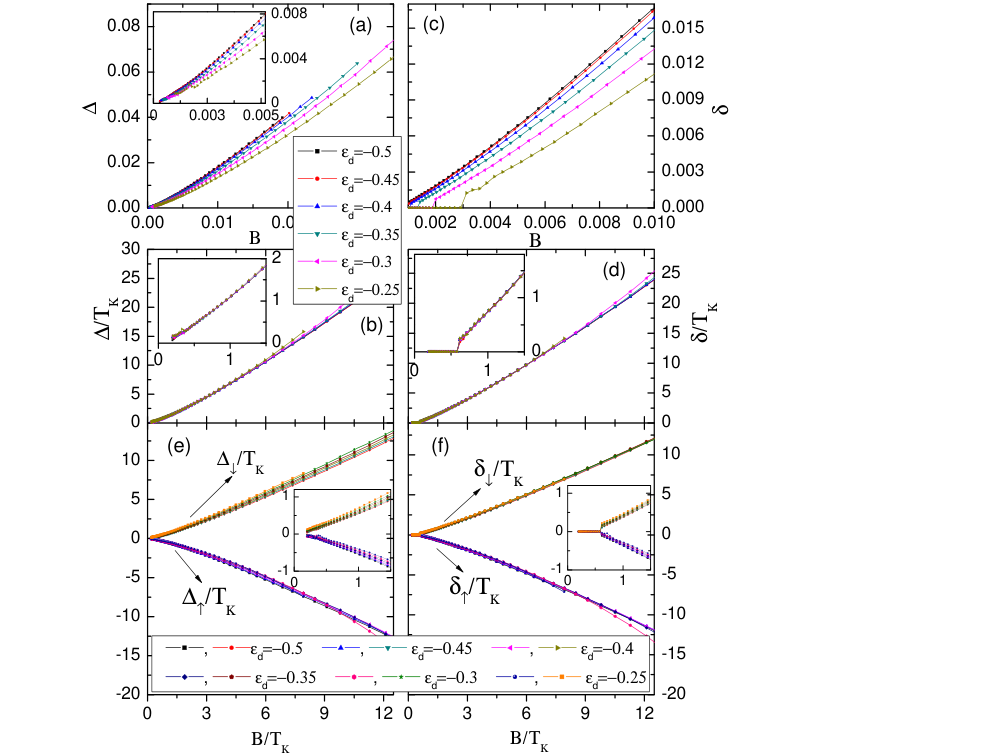
where $\Gamma$ is the whole width of impurity’s energy level. In Fig. 2 (a) and (c), we can see the raw data extracted directly from spectral functions changing gradually along parameter-dependent paths, either in the spin-resolved case or in the spin-average case. It means that if we change some parameters, the evolution of the splittings $\Delta$ and $\delta$ vs $B$ will go along another different path at once. However, after scaling treatment by using Kondo scale $T_{K}$ as the dimensionless unit, these changes of all splittings with increasing $B$ surprisingly go along the same path, as seen in Fig. 2 (b) and (d). Such feature, which is called the scaling characteristic of Kondo effect, is the main subject under detailed investigation in this paper. From the results of Fig.2 (b) and (d), the scaling characteristic will work well for magnetic field $B<8T_{K}$. Whereas with magnetic field getting larger some deviations appear, because the system has been driven closer to the Kondo regime in a larger $B$ region. When the magnetic field $B$ is larger than $10T_{K}$, in which Kondo effect has been suppressed badly and the QD system is out of Kondo regime, obvious deviations in both of splittings $\delta$ and $\Delta$ are exhibited and the scaling theory won’t be obeyed.

In order to clearly show that the system indeed is out of Kondo regime when the magnetic field $B$ is larger than $10T_{K}$, we plot the curves $\Delta_{\uparrow}/B$ and $\Delta_{\downarrow}/B$ versus $B/T_{K}$ by varying $\Gamma$ (see Fig. 3). Here it can be seen clearly that the deviation (i.e.: the non-universal features) are pushed to much larger field $B$ with decreasing $\Gamma$, and in addition no deviations from scaling are found in a low field $B$. As a result, the deviations from scaling found at larger field $B>10T_{K}$ are indeed due to leaving the Kondo regime. In the following, we will mainly focus on the Kondo regime with the magnetic field $B$ less than $10T_{K}$.

Under further investigation of the scaling feature, two differences between the spin-resolved case and spin-averaged case reveal. At first the splitting $\delta$ has an obvious threshold field value at around $0.5T_{K}$, by contrast we can’t see such threshold field in the $\Delta/T_{K}$ vs $B/T_{K}$ curve. This is because the two separated peaks in $A_{\uparrow}(\omega)$ and $A_{\downarrow}(\omega)$ are too close to each other that they overlap and can not be separated in total spectral function. The second difference is about the scaling feature. From (b) and (d) (or by comparison between the insets) we can see the $\delta/T_{K}$ vs $B/T_{K}$ curve presents an linear scaling characteristic, whereas the $\Delta/T_{K}$ vs $B/T_{K}$ curve shows a nonlinear behavior in a low field window.

Next we study the scaling characteristics for the positions of the Kondo peaks $\Delta_{\uparrow}$, $\Delta_{\downarrow}$, $\delta_{\uparrow}$, and $\delta_{\downarrow}$. Fig.2 (e) and (f) show these peak positions ($\Delta_{\sigma}/T_{K}$ and $\delta_{\sigma}/T_{K}$) vs the magnetic field $B/T_{K}$ at different energy level $\varepsilon_{d}$. In approximation, all curves can merge to one curve and the scaling characteristics can hold. However, in detail, all positions of the Kondo peak slightly shift towards the same direction by varying energy level, in the whole magnetic field region (including the weak magnetic field $B<T_{K}$). The deviations are within $0.5T_{K}$ and the deviations in the $\Delta_{\sigma}/T_{K}$-$B/T_{K}$ curves are larger than that in the $\delta_{\sigma}/T_{K}$-$B/T_{K}$ curves. In addition, due to the deviations of the $\Delta_{\sigma}$ and $\delta_{\sigma}$ are towards the same direction, the splittings $\Delta$ ($\Delta=\Delta_{\downarrow}-\Delta_{\uparrow}$) and $\delta$ ($\delta=\delta_{\downarrow}-\delta_{\uparrow}$) can reduce certain parameter-induced deviations and well keep the scaling feature.

Following we adjust Kondo scale $T_{K}$ in another path by varying the coupling strength $\Gamma$, in order to check whether scaling characteristic also works well in this situation. We find out some unusual details reveal in the inset of Fig. 4 (a) although the behavior of splittings with increasing magnetic field shown in Fig. 4 (a) looks much similar like the one in Fig. 2 (b) and (d). Roughly speaking, we can consider the scaling feature as an effective characteristic yet. For the spin-resolved case, ignoring the larger field region where system has been driven closer to or out of Kondo regime, the filed-induced splitting $\Delta/T_{K}$ scales perfectly for magnetic fields all the time. But for the spin-averaged case, we can’t ignore such a fact that evolution of splittings $\delta/T_{K}$ with the increment of $B/T_{K}$ don’t go along exactly the same path, as is seen in inset of (a). Furthermore, we find that such slight deviation always exists as long as the magnetic field is applied in system, and a larger field window is not necessary to reveal this feature along the $\Gamma$ varying path.

The reason for inducing such deviation can be seen in Fig. 4 (b) and (c) where the spectral functions under two specific coupling strength $\Gamma=0.16$ and $0.24$ (denoted by using subscripts $1$ and $2$ respectively) are shown. Since the magnetic field is the only factor inducing Kondo peak splitting as mentioned above, the splitting positions $\Delta_{\uparrow}/T_{K}$ and $\Delta_{\downarrow}/T_{K}$ should be dependent only on field $B$ and $T_{K}$. Along the $\varepsilon_{d}$ varying path, we have seen that $\Delta/T_{K}$ scales perfectly, and here we see this effect also works well along the $\Gamma$ varying path: as shown in Fig.4 (b) and (c), the positions $\Delta_{\sigma}/T_{K}$ of the Kondo peak under two different coupling strength are indeed nearly the same. On the other hand, the positions $\delta_{\uparrow(\downarrow)}/T_{K}$ in the spin-averaged case are not so luck like the one in spin-resolved case. Certain parameters can really influence specific shape of spectral function and the high of Kondo peak (although the Kondo-peak position keeps fixed), and this makes the peak positions of total spectral functions shift a little towards Fermi energy (i.e.: $\omega=0$) with increasing coupling strength $\Gamma$ as shown in Fig.4 (b) and (c). Here is in the place to pinpoint that such effect occurs as long as $B$ is applied, that’s to say the deviation from conventional scaling analysis will be observed under any value of external magnetic field, although this deviation is usually small (within $0.2T_{K}$ in our parameters, see the inset of Fig.4 (a)). This result is consonant with the experimental work by Liu et al[15] in some aspects that the coupling strength can indeed induce deviation from scaling theory, but moreover our work indicates that such deviation occurs all the time along $\Gamma$ varying path, rather than localized in a larger field window.

Another possible way, which explains why $\Gamma$ can induce the small deviation from scaling theory, is to investigate Kondo peak positions shown in Fig. 4 (d) and (e). In present situation, the system remains symmetry ($2\varepsilon_{d}+U=0$) and thus these peak positions keep symmetry as well corresponding to the Fermi energy $\omega=0$. The Kondo-peak positions $\Delta_{\sigma}/T_{K}$ in the spin-resolved case keep nearly the same with changing $\Gamma$ while the magnetic field $B<6T_{K}$, thus $\Delta/T_{K}$-$B/T_{K}$ curve fits the scaling theory well in this field window. In the spin-averaged case, however, the peak position $\delta_{\sigma}/T_{K}$ slightly deviates with changing $\Gamma$. Now the deviation of $\delta_{\uparrow}/T_{K}$ and $\delta_{\downarrow}/T_{K}$ are in the oppositive direction because of the symmetrical peak positions. So this small deviation are not eliminated but enlarged in the splitting $\delta/T_{K}$ and the scaling theory can not hold exactly along the $\Gamma$ varying path.

Since observable deviation of $\delta/T_{K}$ vs $B/T_{K}$ from scaling theory is usually small as is seen in Fig. 4 (a), then such small deviation can be eliminated by averaging out so that scaling analysis can be processed. Next we present a scaling analysis suitable for all field windows within the Kondo regime, for both the spin-resolved case and spin-averaged case.

In Fig. 5 (a) we exhibit the comparison between fitting curves and raw data extracted directly from the spectral functions. Such fitting curves are given by

with the parameters: $a=1.1185,b=1.2627,c=0.03992;d=18.2913,f=2.8572,h=-0.3421$. From Fig. 5 (a) we can see the fitting curves fit numerical data very well in whole magnetic window, including a low field below the conventional threshold value $0.5T_{K}$. Thus we can study some detailed features in a low field with the help of fitting curves. For example, the splitting $\delta$ in spin-averaged case does have a threshold magnetic field at around $0.5T_{K}$ as is seen in (e), and this result is in quantitative agreement with previous theories[10]. What’s more, by using fitting curve $f_{\Delta}(x)$ we find out that in a low magnetic field the curve $\Delta/T_{K}$ vs $B/T_{K}$ likes the power function and the first derivative of $\Delta/T_{K}$ with respect to $B/T_{K}$ is always zero at the zero-field point. When magnetic field $B$ is in the vicinity of $T_{K}$, the curves $f_{\Delta}(x)$ and $f_{\delta}(x)$ exhibit the linear behaviors:

with the parameters: $a_{1}=0.6632,b_{1}=-0.1136;a_{2}=0.7097,b_{2}=-0.3492$. In Fig. 5 (d), we show the curves $f_{\Delta}(x)$, $f_{\delta}(x)$, $y_{\Delta}(x)$, and $y_{\delta}(x)$ together. It clearly shows that $y_{\delta/\Delta}(x)$ is well consistent with $f_{\delta/\Delta}(x)$. In particular, the coefficients $a_{1}$ of the slope of the curve $y_{\delta}(x)$ is $0.6632$, which is nearly the same as $2/3$ derived through Fermi liquid theory.[12]

On the other hand, in the high magnetic field region, the two curves $f_{\Delta}(x)$ and $f_{\delta}(x)$ do not close, whereas they get far away with the increment of $B$. This result is quite surprise. Generally speaking it is believed that splittings $\Delta/T_{K}$ and $\delta/T_{K}$ in the spin-resolved and spin-averaged cases should reach the limit of Zeeman splitting under a large enough magnetic field, thus the two scaling curves $f_{\Delta}(x)$ and $f_{\delta}(x)$ should get closer to one another rather than far away with increasing magnetic field. The key point for the getting far away behavior is that the peak position $\Delta_{\uparrow}$ always falls in the region where its second derivative of spin-down spectral function $A_{\downarrow}$ with respect to $\omega/T_{K}$ is negative (see Fig. 4 (b) and (c)).

In Fig. 5 (b) (c) and (d) we show other scaling features investigated by previous works.[9, 10] $\delta/2B$ is another scaling dimensionless quantity and has been predicted to reach the limit value $1$ (i.e. the splitting of the Kondo peak is equal to the Zeeman splitting) in the large magnetic field $B$ limits.[9, 10] Whereas in recent experiments, such the limit value can be exceeded[8, 15]. In Fig. 5 (b), we show the evolution of $\delta/2B$ vs the magnetic field $B/T_{K}$. The numerical results clearly exhibit that $\delta/2B$ can reach and exceed 1, which is in agreement with the recent experiments[8, 15]. In addition, in the large field window, the curve of $\delta/2B$-$B/T_{K}$ shows the logarithmic behavior.[11] This behavior can clearly be seen in Fig. 5 (c), in which the curve of $\delta/2B$-$ln(B/T_{K})$ is shown.

In conclusion, by using the FDM-NRG method we study the scaling characteristics of the Kondo-peak splittings in a quantum dot system under a magnetic field. Similarly as in the recent experiment,[15] two different ways to adjust the Kondo scale $T_{K}$, via the energy level $\varepsilon_{d}$ and the coupling strength $\Gamma$, are considered. Both splittings $\Delta$ and $\delta$ of Kondo resonant peaks in the spin-resolved spectral function and the total spectral function are investigated in detail. We find that the splitting $\Delta/T_{K}$ in the spin-resolved case always scales perfectly for magnetic fields $B<8T_{K}$ and regardless of the $T_{K}$-adjusted paths. When the magnetic field $B$ is over $10T_{K}$, obvious deviations are exhibited since QD system has been out of the Kondo regime. On the other hand, $\delta/T_{K}$ in the total spectral function, which can be related to the experiments by Liu et al[15], deviates slightly from the conventional scaling theory along the $\Gamma$-varying path. Such result is consonant with the experimental work by Liu et al in some aspects, i.e.: the coupling strength can indeed induce deviation from scaling theory, but moreover our work indicates that such deviation occurs all the time as long as an external magnetic field is applied. Therefore $T_{K}$ is an unsuitable parameter as the scaling dimensionless unit in this situation. Since the deviation in the splitting $\delta/T_{K}$ is usually small, we can still make the scaling analysis for $\delta/T_{K}$. The fitting curves ($f_{\delta}$ and $f_{\Delta}$) for both splittings $\delta/T_{K}$ and $\Delta/T_{K}$ are presented. The fitting curves $f_{\delta}$ has a threshold value at around $0.5T_{K}$, but $f_{\Delta}$ is always non-zero while under the field $B/T_{K}$. In the low field ($B\sim T_{K}$), $f_{\delta}$ exhibits the linear behavior with its slope coefficient $0.663$, consistent with the value of $2/3$ from the Fermi liquid theory. On the large field side, two curves $f_{\delta}$ and $f_{\Delta}$ get apart, and both $\Delta/2B$ and $\delta/2B$ can reach and exceed 1, which is also in agreement with a recent experiments.

We gratefully acknowledge Ning. Hua. Tong for helpful discussion on the NRG method. This work was financially supported by NSF-China under Grants Nos. 10734110, 10821403, and 10974236, China-973 program and US-DOE under Grants No. DE-FG02- 04ER46124.

References

- [1] A. C Hewson, The Kondo Problem to Heavy Fermions (Cambridge University Press, Cambridge, England, 1997)
- [2] T. A. Costi, A. C. Hewson, and V. Zlati, J. Phys. Condens. Matt. 6, 2519(1994)
- [3] D. Goldhaber-Gordon, H. Shtrikman, D. Mahalu, D. Abusch-Magder, U. Meirav, and M. A. Kastner, Nature (London) 391, 156 (1998)
- [4] D. Goldhaber-Gordon, J. Gres, M. A. Kastner, Hadas Shtrikman, D. Mahalu, and U. Meirav, Phys. Rev. Lett. 81, 5225 (1998)
- [5] Y. Meir, N. S. Wingreen, and P. A. Lee, Phys. Rev. Lett. 70, 2601 (1993)
- [6] M. Grobis, I. G. Rau, R. M. Potok, H. Shtrikman, and D. Goldhaber-Gordon, Phys. Rev. Lett. 100, 246601 (2008)
- [7] S. M. Cronenwett, T. H. Oosterkamp, and L. P. Kouwenhoven, Science 281, 540 (1998); C. H. L. Quay, J. Cumings, S. J. Gamble, R. de Picciotto, H. Kataura, and D. Goldhaber-Gordon, Phys. Rev. B 76, 245311 (2007)
- [8] A. Kogan, S. Amasha, D. Goldhaber-Gordon, G. Granger, M. A. Kastner, and Hadas Shtrikman Phys. Rev. Lett. 93, 166602 (2004)
- [9] J. E. Moore and X. G. Wen, Phys. Rev. Lett. 85, 1722 (2000)
- [10] T. A. Costi, Phys. Rev. Lett. 85, 1504 (2000)
- [11] R. M. Konik, H. Saleur, and A. W. W. Ludwig, Phys. Rev. Lett. 87, 236801 (2001); R. M. Konik, H. Saleur, and A. Ludwig, Phys. Rev. B 66, 125304 (2002)
- [12] D. E. Logan, and N. L. Dickens, J. Phys. Condens. Matt. 13, 9713 (2001)
- [13] A. Rosch, T. A. Costi, J. Paaske, and P. Wlfle, Phys. Rev. B 68, 014430 (2003)
- [14] N. Roch, S. Florens, T. A. Costi, W. Wernsdorfer, and F. Balestro, Phys. Rev. Lett. 103, 197202 (2009)
- [15] T. M. Liu, B. Hemingway, A. Kogan, Steven Herbert, and Michael Melloch, Phys. Rev. Lett. 103, 026803 (2009)
- [16] A. Weichselbaum, and J. von Delft, Phys. Rev. Lett. 99, 076402 (2007)
- [17] R. itko, R. Peters, and Th. Pruschke, New. J. Phys. 11, 053003 (2009)
- [18] P. W. Anderson, Phys. Rev. 124, 41 (1961)
- [19] K. G. Wilson, Rev. Mod. Phys. 47, 773 (1975)
- [20] H. R. Krishna-murthy, J. W. Wilkins, and K. G. Wilson, Phys. Rev. B 21, 1003 (1979); H. R. Krishna-murthy, J. W. Wilkins, and K. G. Wilson, Phys. Rev. B 21, 1044 (1979);
- [21] R. Bulla, T. A. Costi, and Th. Pruschke, Rev. mod. Phys. 80, 395 (2008)
- [22] R. Bulla, N. H. Tong, and M. Vojta, Phys. Rev. Lett. 91,170601 (2003)
- [23] F. B. Anders, and A. Schiller, Phys. Rev. Lett. 95, 196801 (2005); F. B. Anders, and A. Schiller, Phys. Rev. B 74, 245113 (2006)
- [24] W. Hofstetter, Phys. Rev. Lett. 85, 1508 (2000)
- [25] R. Peters, Th. Pruschke, and F. B. Anders, Phys. Rev. B 74, 245114 (2006)
- [26] R. Bulla, T. A. Costi, and D. Vollhardt, Phys. Rev. B 64, 045103 (2001)
- [27] EPAPS Document No. E-PRLTAO-99-025733 on the website: http://www.aip.org/pubservs/epaps.html
- [28] W. C. Oliveira, and L. N. Oliveira, Phys. Rev. B 49, 11986 (1994)
- [29] Q. -F. Sun and H. Guo, Phys. Rev. B 64, 153306 (2001); E. Lebanon and A. Schiller, Phys. Rev. B 65, 035308 (2002); S. De Franceschi, R. Hanson, W. G. van der Wiel, J. M. Elzerman, J. J. Wijpkema, T. Fujisawa, S. Tarucha, and L. P. Kouwenhoven, Phys. Rev. Lett. 89, 156801 (2002).
- [30] F. D. M. Haldane, Phys. Rev. Lett. 40, 416 (1978).