On the nature of the X(3872) from QCD
Abstract
We have studied some possible four-quark and molecule configurations of the using double ratios of sum rules, which are more accurate than the usual simple ratios often used in the literature to obtain hadron masses. We found that the different structures ( and tetraquarks and molecule) lead to the same prediction for the mass (within the accuracy of the method), indicating that the alone prediction of the mass may not be sufficient to reveal its nature. In doing these analyses, we also find that (within our approximation) the use of the running , rather than the on-shell mass, is more appropriate to obtain the and meson masses. Using vertex sum rules to roughly estimate the hadronic and radiative widths, we found that the ones of a -like molecule current can be compatible within the errors with the data.
pacs
11.55.Hx, 12.38.Lg , 12.39.-xI Introduction
The nature of the narrow ( 2.3 MeV width) decaying to [1] discovered by BELLE in -decays [2]
and confirmed by BABAR [3], CDF [4] and D0 [5]
in hadronic productions remains puzzling. Different scenarios (four-quark state,
molecule,
large mixing with conventional states) have been evoked in the
literature [6, 7].
In this work we use QCD spectral sum rules (QSSR) (the Borel/Laplace Sum
Rules [8, 9, 10]) in order to test the previous four-quark and molecule
scenarios.
In a previous calculation [11] some of us and our collaborators have
considered the
as being a tetraquark state where the diquark-antidiquark pairs are in
the color configuration.
A priori, the diquark-antidiquark pairs could also be in a color
configuration. This system is expected
to be too weakly bound by a two-body potential but it could be bound by a
four-body potential, such as the one of the
Steiner model [12]. In this work we shall, for the first time,
investigate this configuration using QSSR.
Using QSSR, we shall, also for the first time, analyze the mass and hadronic
width of a -like molecule
11
1
An analogous configuration has been studied within QSSR for light
four-quark states in [13].,
which we shall compare with the ones of the four-quark states.
II The interpolating -currents
In order to study the two-point functions of the meson assumed to be an axial vector meson, The interpolating current which describes the as a diquark-antidiquark system in the color configuration with total is [11]:
| (1) | |||||
while for a diquark-antidiquark in the color sextet () configuration, the interpolating current is:
| (2) | |||||
where are color indices, is the charge conjugation
matrix, denotes a or quark and stands for the
six symmetric Gell-Mann matrices:
.
These tetraquark currents can be compared with the one describing the
state as a molecule:
| (3) | |||||
and as a -like molecule current:
| (4) |
where is the colour matrix.
In the molecule assignement it is assumed that there is an effective local current
and the meson pairs are weakly
bound by a van der Vaals force in a Fermi-like theory with a strength
which has nothing to
do with the quarks and gluons inside each meson.
III The two-point correlator and form of the sum rules
The two-point correlation function associated to the axial-vector current is defined as:
| (5) | |||||
where according to the currents in Eqs. (1),
(2), (3) and (4). The two functions,
and , appearing in Eq. (5) are independent and
have respectively the quantum numbers of the spin 1 and 0 mesons.
Due to its analyticity, the correlation function, , obeys a
dispersion relation:
| (6) |
where is the spectral function. After making an inverse-Laplace (or Borel) transform on both sides, the sum rule and its ratio read:
| (7) |
where is the sum rule variable with being the inverse-Laplace (or Borel) mass. In the following, we shall work with the double ratio of sum rules (DRSR):
| (8) |
to obtain the -meson mass. Defining the coupling of the current with the state through:
| (9) |
and using the minimal duality ansatz: “one resonance” “QCD continuum”, where the QCD continuum comes from the discontinuity of the QCD diagrams from a continuum threshold , the phenomenological side of Eq. (5) can be written as:
| (10) |
where the Lorentz structure projects out the state. The dots denote higher axial-vector resonance contributions that will be parametrized, as usual, by the QCD continuum. Transferring the continuum contribution to the QCD side, the sum rules can be written in a finite energy form as:
| (11) |
IV The QCD expressions of the two-point correlators
The QCD expressions of the spectral densities of the two-point correlator associated to the currents in Eqs. (1) and (3) have been obtained respectively in [11] and [14] and will not be reported here. The expression associated to the current in Eqs. (2) and (4) are new. Up to dimension-six condensates, we can write:
| (12) | |||||
The renormalization improved perturbative expression of the sum rule is given by:
| (13) |
where is the anomalous dimension of the corresponding correlator,
is the first coefficient of the -function for SU(n) flavours,
is the known LO expression and is the radiative correction. By
inspection we observe
that in the ratio of moments defined in
Eq. (11), the corrections disappear and only the radiative
corrections induced
by the anomalous dimensions of the currents survive.
In the double ratios of sum rules (DRSR) which we shall use in this paper, this
induced
radiative correction will also disappear to as the different
currents studied
(which have all the same Lorentz structure) have the same anomalous dimensions.
Therefore, we expect that,
although we work in leading order of the QCD expressions, our results for the
ratios of
masses are accurate up to order for the perturbative contributions.
IV.1 four-quark current
For the current in Eq. (2), we get to lowest order in :
| (14) |
where: are respectively the charm quark mass, gluon condensate, light quark and mixed condensates; indicates the violation of the four-quark vacuum saturation. The integration limits are given by:
| (15) |
where is the -quark velocity:
| (16) |
IV.2 -like molecule current
V Calibration of the method from and choice of
Using the QSSR method, one usually estimates the mass, from the ratio:
| (18) |
where is the spectral density associated to the vector current:
| (19) |
The QCD expression of the vector correlator is known in the literature [8] including the condensates [10]. The full expression of the exponential moments is given in [15] and its expansion in can be found in [16]. For the numerical analysis we shall introduce the renormalization group invariant quantities [17]:
| (20) |
where is the first coefficient of the function for flavours. We have used the quark mass and condensate anomalous dimensions reported in [10]. We shall use the QCD parameters in Table 1. At the scale where we shall work, and using the parameters in Table 1, we deduce:
| (21) |
which controls the deviation from the factorization of the four-quark condensates. We shall not include the term discussed in [18, 19],which is consistent with the LO approximation used here as the latter has been motivated by a phenomenological parametrization of the larger order terms of the QCD series.
| Parameters | Values | Ref. |
|---|---|---|
| MeV | [20, 1] | |
| MeV | [21, 10] | |
| GeV2 | [22, 23, 24] | |
| GeV4 | [20, 25, 26, 27, 28, 29, 15, 30, 31] | |
| GeV6 | [20, 25, 22] | |
| GeV | [10, 21, 32, 1, 30, 33] |
Including the gluon condensate, we show in Fig. 1a the -behaviour of , for a given GeV, from which the pQCD expression of the spectral density starts to be seen experimentally.


From Fig. 1a we see that the gluon contribution plays an important role in stabilizing the result. In Fig. 1b we show the behaviour of for two values of . We see that the results are very stable against . One can deduce from Fig. 1a and Fig. 1b that one can better reproduce the experimental value of using the running mass rather than the on-shell mass . This feature had already been noticed in [33, 30], where a better convergence of the QCD perturbative series was found when working with the mass. Therefore, in the following we shall only consider the running mass. We have checked that the use of the on-shell mass does not affect our result from the double ratio of sum rules as it was intuitively expected.
VI from the double ratios of sum rules (DRSR)
VI.1 The tetraquark
Using QSSR, one can usually estimate the mass of the -meson, from the ratio analogue to the one in Eq. (18), where is related to the spectral densities obtained from the currents (1) and (2) respectively. The component of the mass has been studied with the help of the current (1). At the sum rule stability point and using a slightly different (though consistent) set of QCD parameters than in Table 1, one obtains with a good accuracy [11]:
| (22) |
and the correlated continuum threshold value fixed simultaneously by the Laplace and finite energy sum rules (FESR) sum rules:
| (23) |
is in good agreement (within the errors) with the experimental candidate [1]:
| (24) |
while the relative low value of indicates that the next radial excitation of the -meson can be in the range:
| (25) |
This low value of suggests that the resonance may be difficult to separate from the QCD continuum and suggests also that it can be a wide resonance. Although the agreement with the experimental data is remarkable, the result may not be sufficient to provide a definite statement on the quark substructure of the -meson.
over tetraquark
A better understanding of the nature of the , for discriminating different proposals, requires a more precise determination of . This can be reached by considering the double ratio (DR) of the sum rules (DRSR) [16, 24, 34, 35, 36, 37]:
| (26) |
These quantities are less sensitive to the choice of the heavy quark masses, to the perturbative radiative corrections and to the value of the continuum threshold than the simple ratios and in Eq. (18) and (22). Fixing [11] we show in Fig. 2a the -behaviour of (continuous line) for two values of . One can notice that the result is very stable against the -variation in a large range for GeV-2 . We show in Fig. 2b its -behaviour (continuous line) for a given GeV-2 and GeV. We deduce:
| (27) |
with a negligible error, which shows that, from a QCD spectral sum rules approach, the can be equally described by the currents in Eqs. (1) and (2).


VI.2 molecule over tetraquark
We can also work with the double ratio:
| (28) |
by using the spectral densities for the current (3). In Fig. 2a we also show the double ratio (dashed line) for and for two values of , while we show in Fig. 2b its -behaviour (dashed line) for a given GeV-2 and GeV. One can deduce from the previous analysis:
| (29) |
also with a negligible error.
VI.3 -like-molecule over the tetraquark
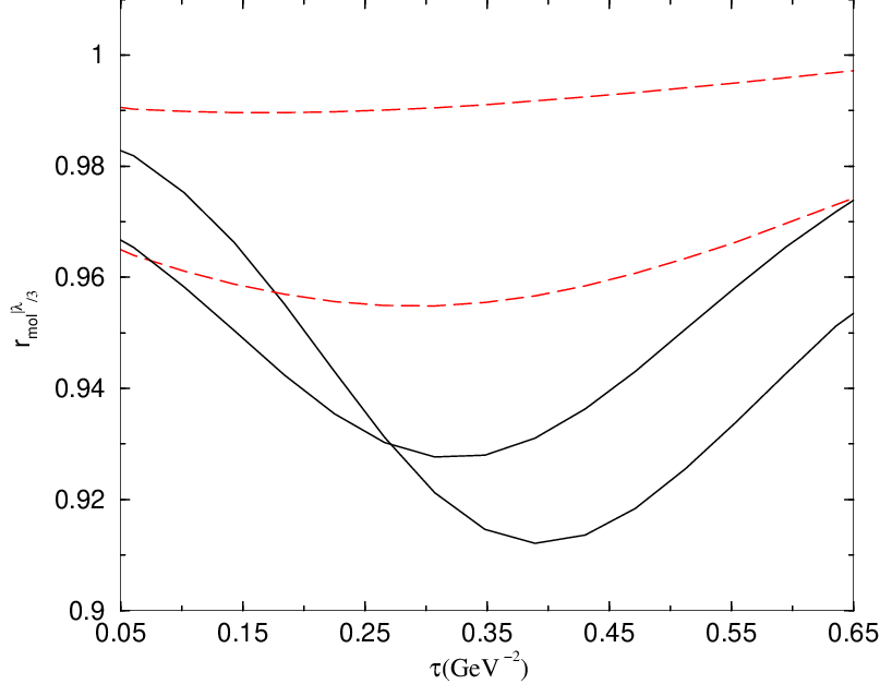
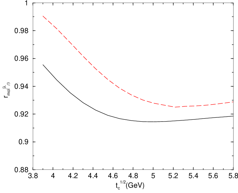
Using approaches similar to the previous ones, we study the ratio of the -like molecule over the tetraquark one. We show the analysis in Fig. 3 from which one can deduce at the and stability regions:
| (30) |
where the errors come from the stability regions and 22 2 The analysis of the ratio between the -molecule -like current and mass is not conclusive within our approximation due to the absence of a stability region. The appearance of an inflexion point favors a lower value of the -molecule mass. However, analyzing the ratio of the 4-quark over the 2-quark correlators which do not necessarily optimize at the same -values may be inappropriate..
VI.4 Comments on the results
Our analysis has shown that the three substructure assignements for the
-meson ( and tetraquarks and molecule) lead
to (almost) the same mass predictions within the accuracy of the approach.
Therefore, a priori, the alone study of the -mass cannot reveal
its nature if it is mainly composed by these substructures.
From the previous analysis we observe that the distance between the
continuum threshold (about 4 GeV) and the resonance masses (see e.g. the ratio
in Fig. 2)
is relatively small. This indicates that the separation between the resonance
and the continuum may be difficult
to achieve. This feature is also signaled by the (almost) absence of the
so-called sum rule window
(a compromise region where the resonance dominates over the continuum
contribution and where the QCD OPE is
convergent) when one extracts the absolute mass of the mass.
Then, as in the analysis of the wide
[38] and hybrid or some other large width states
[10, 39], we expect that the
33
3
In a particular two-body potential model, one might expect that the
tetraquark state can be
weakly bound due to the repulsive force between the two quarks, but this may
not necessarily be true for a more
more general potential [12].
and, to a lesser extent, the four-quark or molecule
states can be wide or/and weakly bound.
The analysis of the -like molecule mass in Eq.
(30) shows that it can be lower
than the other configurations studied previously.
In order to get a deeper understanding of the properties of these states,
we shall, in what follows, compute their hadronic widths.
VII Can the -meson hadronic width reveal its nature ?

One can study the decays and using vertex sum rules [40], where the and can be assumed to come from the and mesons using vector meson dominance (VDM) 44 4 This approach assumes implicitly that the decay occurs through a direct coupling of the -meson to and mesons where some eventual rescattering contributions (which could be important) have been neglected.. In so doing, one works with the three-point function:
| (31) | |||||
associated to the -meson , to the vector mesons and to the -meson .
VII.1 The tetraquarks and molecule
In the case of the three -currents (, tetraquarks and molecule) discussed previously, the lowest order and lowest dimension correction (fall apart) QCD diagrams are shown in Fig. 4. An estimate of the coupling in [14, 40] indicates that if the is a pure tetraquark or a molecule state, one would obtain:
| (32) |
which would correspond to a width:
| (33) |
Doing an analogous analysis if the is a tetraquark state, one also
obtains a similar value.
These previous results are too big compared with the data upper bound [2]:
| (34) |
VII.2 The -like molecule


Another possibility is to study the -like molecule current. In contrast to to the case of previous currents, the leading order contribution to the three-point function is due to one gluon exchange in Fig. 5. The exact evaluation of these diagrams are technically involved. However, a rough approximation by including loop factors 55 5 A similar estimate has been done in [13] for explaining the too small width of the if it is a four-quark or molecule state. leads to the coupling:
| (35) |
where we have used . This would corresponds to a width :
| (36) |
which satisfies the previous experimental upper bound. Due to the rough approximation used in the estimate, we may expect that the result is known within a factor 2 .
A similar rough approximation can be made to evaluate the radiative decay width . This decay was studied in ref. [41] considering the as having charmonium and molecular () components. In the case that is a pure tetraquark or a molecule state, one would obtain within :
| (37) |
Therefore, using also in this case the rough approximation
| (38) |
we get within a factor 2:
| (39) |
which also satisfies the experimental upper bound. From the results in Eqs. (36) and (39) we would get:
| (40) |
Taking into account the rough approximation of a factor 2 used to estimate each width, this result can be consistent with the experimental value [42]:
| (41) |
VIII Conclusions
We have studied the mass of the using double ratios of sum rules,
which are more accurate
than the usual simple ratios used in the literature. We found that the different
proposed configurations
( and tetraquarks and molecule) lead to (almost)
the same mass predictions
within the accuracy of the method [see Eqs. (27) and (29)],
indicating that the predictions
of the -meson mass is not enough to reveal its nature. However, the (relatively)
small distance between the
resonance mass and the continuum threshold in the QSSR analysis and also the
(almost) absence of the
sum rule window, indicate that these and tetraquarks and
molecule states can be
wide or weakly bound. These observations are also supported by their large
hadronic decay widths from vertex sum rules
analysis given in Eq. (33) [40].
Among these different proposals, the only eventual possibility which can lead
to a with narrow hadronic and radiative widths consistent within the errors
with the present data,
is the choice of the -like molecule current given in Eq. (4).
Sharper tests of the previous results can be done from an explicit evaluation of the
QCD vertex function and from a more precise experimental measurements of the
the ratio in Eq. (41). In this case, some eventual mixing among different currents
(see e.g. [14, 41]) may help to improve the agreement between theory and experiment.
IX Acknowledgements
M. Nielsen would like to thank R.D. Matheus and C.M. Zanetti for useful discussions and for some partial collaborations, and the LPTA-Montpellier for the hospitality where this work has been initiated. This work has been partly supported by the CNRS-FAPESP program, by CNPq-Brazil and by the CNRS-IN2P3 within the project Non-perturbative QCD and Hadron Physics.
References
- [1] For a review, see e.g. PDG 08, C. Amsler et al., Phys. Lett. B 667 (2008) 1.
- [2] S.-K. Choi et al. [Belle Collaboration], Phys. Rev. Lett. 91, 262001 (2003).
- [3] B. Aubert et al. [BaBar Collaboration], Phys. Rev. D 71, 071103 (2005).
- [4] D. Acosta et al. [CDF II Collaboration], Phys. Rev. Lett. 93, 072001 (2004);
- [5] V. M. Abazov et al. [D0 Collaboration], Phys. Rev. Lett. 93, 162002 (2004);
- [6] For reviews, see e.g., E. S. Swanson, Phys. Rept. 429, 243 (2006); J. M. Richard, talk given at QCD 05 (Montpellier 4-8th July 2005), hep-ph/0601043.
- [7] For a review, see e.g. M. Nielsen, F. S. Navarra, S. H. Lee, arXiv:0911.1958.
- [8] M.A. Shifman, A.I. and Vainshtein and V.I. Zakharov, Nucl. Phys. B147, 385 (1979).
- [9] L.J. Reinders, H. Rubinstein and S. Yazaki, Phys. Rept. 127, 1 (1985).
- [10] For a review and references to original works, see e.g., S. Narison, QCD as a theory of hadrons, Cambridge Monogr. Part. Phys. Nucl. Phys. Cosmol. 17, 1-778 (2002) [hep-h/0205006]; QCD spectral sum rules , World Sci. Lect. Notes Phys. 26, 1-527 (1989); Acta Phys. Pol. B26 (1995) 687; Riv. Nuov. Cim. 10N2 (1987) 1; Phys. Rept. 84, 263 (1982).
- [11] R.D. Matheus, S. Narison, M. Nielsen, J.M. Richard, Phys. Rev. D75, 014005 (2007).
- [12] See e.g. K. Terasaki, arXiv:1005573 [hep-ph]; J.M. Richard, QCD 10 (July 2010-Montpellier) and private comunication.
- [13] S. Narison, Phys. Lett. B175, 88 (1986).
- [14] R. D. Matheus, F. S. Navarra, M. Nielsen, C. M. Zanetti, Phys. Rev. D80, 056002 (2009).
- [15] J.S. Bell and R.A. Bertlmann, Nucl. Phys. B 227, (1983) 435; R.A. Bertlmann, Acta Phys. Austriaca 53, (1981) 305; R.A. Bertlmann and H. Neufeld, Z. Phys. C 27 (1985) 437.
- [16] S. Narison, Phys. Lett. B 387 (1996) 162.
- [17] E.G. Floratos, S. Narison and E. de Rafael, Nucl. Phys. B 155 (1979) 155.
- [18] K. Chetyrkin, S. Narison and V.I. Zakharov, Nucl. Phys. B 550 (1999) 353; S. Narison and V.I. Zakharov, Phys. Lett. B 522, (2001) 266; S. Narison and V.I. Zakharov, Phys. Lett. B 679, (2009) 355.
- [19] For reviews, see e.g.: V.I. Zakharov, Nucl. Phys. Proc. Suppl. 164 (2007) 240; S. Narison, Nucl. Phys. Proc. Suppl. 164, 225 (2007).
- [20] S. Narison, Phys. Lett. B 673 (2009) 30.
- [21] For reviews, see e.g.: S. Narison, Phys.Rev. D 74 (2006) 034013; arXiv:hep-ph/0202200; Phys. Lett. B 216 (1989) 191; Phys. Lett. B 358 (1995) 113; Phys. Lett. B 466 (1999) 345; S. Narison, H.G. Dosch, Phys. Lett. B 417 (1998) 173; S. Narison, N. Paver, E. de Rafael and D. Treleani, Nucl. Phys. B 212 (1983) 365; S. Narison, E. de Rafael, Phys. Lett. B 103 (1981) 57; C. Becchi, S. Narison, E. de Rafael, F.J. Yndurain, Z. Phys. C 8 (1981) 335.
- [22] Y. Chung et al.Z. Phys. C 25 (1984) 151; H.G. Dosch, Non-Perturbative Methods (Montpellier 1985); H.G. Dosch, M. Jamin and S. Narison, Phys. Lett. B 220 (1989) 251.
- [23] B.L. Ioffe, Nucl. Phys. B 188 (1981) 317 , B 191 (1981) 591; A.A.Ovchinnikov and A.A.Pivovarov, Yad. Fiz. 48 (1988) 1135.
- [24] S. Narison, Phys. Lett. B 210, 238 (1988); Phys. Lett. B 605, 319 (2005).
- [25] G. Launer, S. Narison and R. Tarrach, Z. Phys. C 26 (1984) 433.
- [26] S. Narison, Phys. Lett. B 300 (1993) 293; ibid B 361 (1995) 121.
- [27] R.A. Bertlmann, G. Launer and E. de Rafael, Nucl. Phys. B 250 (1985) 61; R.A. Bertlmann et al., Z. Phys. C 39 (1988) 231.
- [28] F.J. Yndurain, hep-ph/9903457.
- [29] S. Narison, Phys. Lett. B 387 (1996) 162.
- [30] S. Narison, arXiv:1004.5333 [hep-ph] and references therein.
- [31] S. Narison, Phys. Lett. B361, 121 (1995); Phys.Lett. B624 (2005) 223.
- [32] S. Narison, Phys. Lett. B 197 (1987) 405; Phys. Lett. B 341 (1994) 73; Phys. Lett. B 520 (2001) 115.
- [33] B.L. Ioffe and K.N. Zyablyuk, Eur. Phys. J. C 27 (2003) 229; B.L. Ioffe, Prog. Part. Nucl. Phys. 56 (2006) 232.
- [34] S. Narison, Phys. Lett. B 322 (1994) 327.
- [35] S. Narison, Phys. Lett. B 337 (1994) 166; Phys. Lett. B 668 (2008) 308.
- [36] S. Narison, Phys.Rev. D 74 (2006) 034013; Phys. Lett. B 358 (1995) 113; Phys. Lett. B 466 (1999) 34.
- [37] R.M. Albuquerque, S. Narison, M. Nielsen, Phys. Lett. B 684 (2010) 236; R.M. Albuquerque, S. Narison, Phys. Lett. B 694 (2010) 217.
- [38] S. Narison, G. Veneziano, Int. J. Mod. Phys. A 4 (1989) 2751; S. Narison, Nucl. Phys. B 509 (1998) 312; Phys. Rev. D 73 (2006) 114024.
- [39] S. Narison, Phys. Lett. B 675 (2009) 319.
- [40] F. Navarra and M. Nielsen, Phys. Lett. B 639 (2006) 272.
- [41] M. Nielsen, C.M. Zanetti, arXiv:1006.0467 [hep-ph].
- [42] K. Abe et al. [Belle Collaboration], hep-ex/0505037, hep-ex/0505038.