Vertices of closed curves in Riemannian surfacesThanks: Supported by NSF Grant DMS-0336455, and CAREER award DMS-0332333.
Abstract.
We uncover some connections between the topology of a complete Riemannian surface and the minimum number of vertices, i.e., critical points of geodesic curvature, of closed curves in . In particular we show that the space forms with finite fundamental group are the only surfaces in which every simple closed curve has more than two vertices. Further we characterize the simply connected space forms as the only surfaces in which every closed curve bounding a compact immersed surface has more than two vertices.
Key words and phrases:
Four vertex theorem, Riemannian surface, surface of constant curvature, space form, hyperbolic surface, geodesic curvature.1991 Mathematics Subject Classification
Primary: 53C20, 53C22; Secondary: 53A04, 53A05.1. Introduction
In this paper we study the relation between the topology of a complete Riemannian surface and the minimum number of vertices, i.e., critical points of geodesic curvature, of closed curves in . Our prime motivation here is the classical theorem of Kneser [25, 29], which states that any simple closed curve in Euclidean plane has at least four vertices. It is known that this result also holds in the sphere and hyperbolic plane , since the stereographic projection and the inclusion map of the Poincaré disk preserve vertices [26, 9]. Further, it follows from another classical result due to Möbius [28, 39] that any simple closed curve in the projective plane has at least three vertices. We show that, up to a rescaling, these are the only surfaces where every simple closed curve has more than two vertices:
Theorem 1.1.
The only complete Riemannian surfaces where every simple closed curve has more than two vertices are the space forms with finite fundamental group.
Thus the simply connected space forms are the only complete Riemannian surfaces where Kneser’s four vertex theorem holds, and real projective planes are the only other surfaces where every simple closed curve has at least three vertices. Another classification result we obtain in this work uses the extension of Kneser’s theorem to self-intersecting curves by Pinkall [34] who showed that every closed curve in (and hence and ) which bounds a compact immersed region must have at least four vertices. Our next theorem shows that this property also characterizes the simply connected space forms:
Theorem 1.2.
The only complete Riemannian surfaces where every closed curve which bounds a compact immersed surface has more than two vertices are the simply connected space forms.
Finally one may ask what are all surfaces which satisfy the condition of the last theorem if the word “immersed” is replaced by “embedded”. Obviously, surfaces of the above theorems would then fall into that category, but there are more examples:
Theorem 1.3.
The only complete Riemannian surfaces where every closed curve which bounds a compact embedded surface has more than two vertices are orientable space forms of genus zero, flat tori, and rescalings of .
We recall that an orientable surface of genus zero is one that is homeomorphic to minus a totally disconnected subset [37]. The above theorems are proved in the next three sections below. The proofs of Theorems 1.1 and 1.3 employ some basic curve shortening and certain perturbation results for closed geodesics or horocycles in hyperbolic surfaces. An important lemma utilized here is a result of Jackson [24] who showed that Kneser’s four vertex property holds only in surfaces with constant curvature. The proof of Theorem 1.2 also uses this lemma, together with an explicit example of a rather remarkable cylindrical curve which has only two vertices but bounds a compact immersed surface (Figure 5). A general result for perturbing closed geodesics to curves with only two vertices is discussed in the appendix.
Four vertex theorems have spawned a vast and diverse literature since the first version of the theorem was proved in 1909 by Mukhopadhyaya [30], who showed that convex planar curves have four vertices. This is the only version mentioned in nearly all differential geometry textbooks, with the exceptions of [18, 29] where the more general theorem of Kneser is discussed, see also [23, 31, 20]. Pinkall’s paper [34] and related work [48, 7] offer other more general proofs as well, based on a number of ideas. For more recent proofs see [1, 45] which use curvature flow and Sturm theory. Another recent development is concerned with a converse of Kneser’s theorem [10, 15]. There are also interesting generalizations to space curves [41, 49, 46], connections with contact geometry [2, 50], polygonal analogues [33], and a version for surfaces with boundary [14]. See [36] for a physical application, and [13, 32] for some more references and historical remarks.
2. Proof of Theorem 1.1
We begin by recording the result of Jackson mentioned above:
Lemma 2.1 ([24]).
Let be a Riemannian surface with curvature and let be a point of . Suppose that is not a stationary point of , i.e, . Then there exists an such that for all , the metric circle of radius centered at has only two vertices.∎
Thus we may confine our attention to complete Riemannian surfaces of constant curvature , or -dimensional space forms, as far as proving Theorem 1.1 is concerned. Furthermore, we may assume that is not simply connected due to the following fact: let denote the unit sphere and be the Poincaré half-plane with its standard metric of constant curvature ; then we have:
Lemma 2.2 ([26]).
The stereographic projection and the inclusion map preserve the sign of the derivative of the geodesic curvature of curves.∎
Thus Kneser’s theorem holds in all simply connected -dimensional space forms. The property of the stereographic projection mentioned above was already known to Kneser [25], and the property of the inclusion map for the Poincaré disk was proved by Maeda [26]; but the Poincaré disk and half-plane are equivalent up to a Möbius transformation, which establishes the corresponding fact for the Poincaré half-plane, since Möbius transformations preserve vertices [34, 20]. Essentially, these observations are consequences of the fact that the stereographic projection and the inclusion map of the upper half-plane send circles to circles, and the vertices occur when the curve has third order contact with its osculating circle.
It remains to consider non-simply connected -dimensional space forms . We may assume, after a rescaling, that the curvature of is , , or . Then by the Hopf-Killing theorem [44, 38], where , , or and is a discreet subgroup of isometries of which acts freely and properly discontinuously on . In particular, the projection is a Riemannian covering map. We also recall that is isometric to the fundamental group . Indeed, for any point , with , and closed curve with , if is the lifting of with , then there exists a unique element such . This correspondence, which will be utilized a number of times below, establishes the isomorphism between and .
2.1. The elliptic case
If , then is the real projective plane . By a theorem of Möbius [28, 39], see Note 2.8 below for other references, any simple closed noncontractible curve in has at least three inflection points, i.e., points where the geodesic curvature vanishes. But there must be at least one vertex between every pair of inflections. Thus must have at least three vertices. On the other hand, if is contractible, then it lifts to a pair of simple closed curves in , each of which must have four vertices by Kneser’s theorem. Since the covering map is one-to-one on each of these curves, it then follows that must have at least four vertices. So we conclude then that all simple closed curves in must have at least three vertices. (Note that in a nonorientable surface, the geodesic curvature in only well-defined locally and up to a sign; however, this is enough to allow one to talk about vertices and inflection points.)
In the remaining cases we construct explicit examples of simple closed curves with only two vertices, by perturbing geodesics or horocycles of .
2.2. The parabolic case
If , then where there are exactly four types of possibilities for corresponding to the cases of cylinder, twisted cylinder, torus, or Klein bottle [44]. In each of these cases contains a simple closed geodesic , as may be easily seen by looking at the fundamental region of these surfaces which is either a rectangle or an infinite strip in . Let be a parametrization of by arclength (where denotes the length of ), and be a lifting of to . Then traces a line which we may assume to be the -axis. Let be the unique element such that . Then is either the “translation” or the “glide reflection” and we define, respectively,
for some . Then the image of is invariant under the action of . Consequently, if denotes the covering map, then traces a smooth closed curve in with only one or two vertices. Further note that, as , converges to , and consequently converges to with respect to the -norm. So since is simple, it follows that will be simple as well for sufficiently small .
2.3. The hyperbolic case
If , or is a hyperbolic surface, we need to establish a basic structure theorem first. Recall that an end of a surface is a nested sequence of subsets which eventually lie outside any given compact subset. Each element of this sequence is called an end representative, and two ends are equivalent if each representative of one end lies in a representative of the other. A cusp of a hyperbolic surface is an end with a representative which is isometric to a representative of the “thin” end of the parabolic cylinder where is generated by the parabolic translations ; more explicitly, a cusp representative may be defined as
for some . Alternatively, a cusp may be visualized as an end of the tapering surface of revolution in known as the pseudosphere.
Proposition 2.3.
Every non-simply connected complete hyperbolic surface contains a simple closed geodesic or a cusp.
In the special case where the surface is orientable and has finite Euler characteristic, the above proposition follows from a result in the recent book of Borthwick [6, Prop. 2.16]. With the aid of this result, and some curve shortening, we give the more general proof which we seek. First we need to establish the following lemma. If were orientable, this lemma would follow from basic results on curve shortening flow by curvature [17, 8]; however, when is not orientable, the geodesic curvature is not well-defined along the entire curve; hence we use the “disk flow” method devised in [19] which does not require orientability.
Lemma 2.4.
Let be a complete Riemannian surface and be a simple closed curve of length in . Suppose that is not isotopic to a point and the set of all curves in the isotopy class of whose lengths are bounded above by are confined to a compact region of . Then is isotopic to a simple closed geodesic.
Proof.
If is compact, the lemma follows immediately from [19, Thm. 1.8]. But the proof of [19, Thm. 1.8] shows that compactness is needed only so that one can apply Ascoli’s theorem to conclude that any length non-increasing homotopy has a convergent subsequence. Of course one may draw the same conclusion as long as is confined to a compact subset of , which we assume is the case. ∎
Next we use the previous lemma to establish another basic fact:
Lemma 2.5.
Every complete non-orientable Riemannian surface contains a simple closed geodesic, which has a tubular neighborhood homeomorphic to a Möbius strip.
Proof.
If a complete Riemannian surface is nonorientable then it must contain a Möbius band . Let be a smooth simple closed curve which is a retraction of . By the isotopy extension lemma [22], if is any curve in which is isotopic to , then will also have a neighborhood which is homeomorphic to a Möbius band and retracts onto . This yields the following two observations. First, is not isotopic to a point, because every surface is locally orientable. Second, no curve homotopic to may be disjoint from . This is due to the fact that there exists a smooth curve homotopic to which intersects only once, see Figure 1.

Next note that any curve homotopic to will be homotopic to as well. Suppose now, towards a contradiction, that is disjoint from . Then, if denotes the intersection number, we have
by the invariance of intersection number under homotopy [22]. Thus, . This shows that any length nonincreasing isotopy of must be confined within a compact region of (if length of is , then this region would consist of points of which are within a distance of ). It follows then, via Lemma 2.4, that is isotopic to a simple closed geodesic. ∎
We need only one other basic result before proving Proposition 2.3. A hyperbolic cylinder is the quotient where is generated by the hyperbolic translations . Thus a hyperbolic cylinder contains a simple closed geodesic, i.e., the image of the positive half of the -axis, which cuts the cylinder in half. Following Borthwick [6] we define a funnel, as one of these halves. We say that a surface is topologically finite if it is homeomorphic to a compact surface minus a finite set of points.
Lemma 2.6 ([6]).
Every non-simply connected noncompact complete orientable hyperbolic surface with finite topology has a cusp or funnel end.
Proof.
If our hyperbolic surface is homeomorphic to an annulus, or, equivalently, is orientable and has only one generator, then that generator is conjugate to either a parabolic or hyperbolic translation of , which we defined above. Consequently is isometric to either the parabolic cylinder or hyperbolic cylinder, in which case has a cusp or funnel end respectively, and we are done. On the other hand, if is not homeomorphic to an annulus (and is not simply connected), then will be “nonelementary” and the proof follows from [6, Thm. 2.13] which classifies the ends of nonelementary geometrically finite orientable hyperbolic surfaces. To apply this classification result, we just need to note that since is topologically finite, it is “geometrically finite” as well [6, Thm. 2.10], i.e., is finitely generated, or, equivalently, the fundamental region of is a finite-sided convex polygon in . ∎
Now we are ready to prove Proposition 2.3:
Proof of Proposition 2.3.
By Lemma 2.5 we may suppose that our surface, say , is orientable. It is well-known that every compact non-simply connected orientable surface contains a simple closed geodesic, e.g., this follows from Lemma 2.4; or see [38, Sec. 9.6] for the hyperbolic case. So we may also suppose that is noncompact. Then, if has finite topology, by Lemma 2.6, one of the ends of must be a “cusp” or a “funnel” [6]. In either case we would be done since, by definition, funnels are bounded by simple closed geodesics. So it remains to consider the case where has infinite topology, although all we need is that have at least four ends. Then we show that must have a simple closed geodesic as follows.
By the generalized Jordan curve theorem, any simple closed curve divides into two components. Choose so that each of the components of contains at least two ends of , and is rectifiable. Then let be a length nonincreasing isotopy of , e.g., as defined by Hass and Scott [19, Thm. 1.8]. Note that, by the isotopy extension lemma [22], the topology of does not depend on . Let be a continuous choice of a component of , and be an end representative of which does not contain all ends of that are in . Then cannot be contained entirely in for any time , because then would be disjoint from some of the ends of . Now let be another end representative such that the distance of from is bigger than were is the length of . Then for all .
Similarly, for each end of we may choose an end representative which will always be disjoint from . Then the complement of all these end representatives is a compact subset of which contains for all , and so we may apply Lemma 2.4 to complete the proof. ∎
Having proved Proposition 2.3, we may now proceed with the rest of the proof of Theorem 1.1 by considering the following two cases:
2.3.1.
If our hyperbolic surface contains a cusp, then it contains a horocycle, i.e., a simple closed curve which lifts to a horizontal line . Then let be the perturbation of given by
see Figure 2.

Recall that there is a unique element , given by , which in this case is the parabolic translation . Further, as we argued in Section 2.2, since is also invariant with respect to , the projection is a smooth closed curve in with only two vertices for any , by Lemma 2.2. Furthermore, again as , converges to with respect to the norm. Thus, since is simple, will be simple as well.
2.3.2.
If contains a simple closed geodesic , then it lifts to a geodesic . We may assume that traces the upper half of the -axis in its positive direction, and . Then (recall that the hyperbolic distance of from is given by ). As before, let be the (unique) element such that . Then is either the hyperbolic translation or the glide reflection , depending on wether or not small tubular neighborhoods of are orientable. So there are two cases to consider:
If is the hyperbolic translation (i.e., a tubular neighborhood of in is orientable), let
see Figure 3.

Note that , i.e., the image of is invariant under the action of . Thus is a smooth closed curve in , and choosing sufficiently small we can make sure that is simple as we argued in Section 2.2. Finally note that has only two vertices on the interval . Thus, the projection of will have only two vertices, again by Lemma 2.2.
If is the glide reflection (i.e., no neighborhood of in is orientable) let
Then the image of is invariant under the action of and again yields the desired curve for small , which completes the proof of Theorem 1.1.
We record below the last part of the proof for future reference:
Lemma 2.7.
Any closed geodesic or horocycle in a hyperbolic surface is -close to a closed curve with no more than two vertices. ∎
Note 2.8.
The theorem of Möbius mentioned above is equivalent to the statement that every simple closed curve in which is symmetric with respect to the antipodal reflection () has at least six inflection points. Since the antipodal reflection switches the sign of geodesic curvature, the number of inflection points of must be where is odd. So, it is enough to show that has more than two inflections. In this sense, the theorem of Möbius may be viewed as a special case of the “tennis ball theorem” [2, 3, 1] which proves the existence of at least four inflections for curves which bisect the area of . The latter result in turn follows from a theorem of Segre [42] who proved that any simple closed curve on which contains the origin in its convex hull must have at least four inflection points. Another proof of Segre’s theorem may be found in [51]. For other refinements or results related to the theorem of Möbius see, [40, 47, 35].
3. Proof of Theorem 1.2
Let be a complete Riemannian surface satisfying the hypothesis of Theorem 1.2. By Lemma 2.1, and after a rescaling, we may again assume that has constant curvature , , or which result in the following three cases respectively:
3.1. The elliptic case
Recall that here is the real projective plane . In this case we may construct an explicit example of a curve with only two vertices, which bounds an immersed compact surface, as shown in Figure 4.
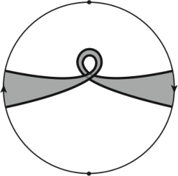
In this picture, is represented as a hemisphere of , say the northern hemisphere, with the antipodal points on its boundary, or the equator, identified, and we are looking at this hemisphere from “above” (i.e., in a direction orthogonal to the plane of the equator). Alternatively, the above picture may be regarded as that of a unit disk, and then we may transfer the depicted region to a hemisphere via a stereographic projection, which preserves the number of vertices by Lemma 2.2. Note that the points where the curve intersects the boundary of the hemisphere are inflection points.
3.2. The parabolic case
In this case where has at most two generators one of which must be a translation or a glide reflection [44]. But the composition of two glide reflections is a translation. Thus must contain a subgroup generated by a translation. Then the projection yields a covering of by a cylinder. Thus it is enough to show that every flat cylinder contains a closed curve with only two vertices which bounds a compact immersed surface. Then the covering map yields the corresponding examples in all other topological types of flat surfaces (the twisted cylinder, the torus, and the Klein bottle).

So we may suppose that is a flat cylinder, i.e., which is the quotient of modulo the horizontal translations . Alternatively, we may think of as the fundamental region with its right and left hand sides identified. Then the curve we seek is depicted in the left hand side of Figure 5, and the picture on the right shows a lifting of that curve in . Note that the curve on the cylinder bounds a compact immersed surface. Thus we only need to check that the given curve has only two vertices. Indeed the curve on the right is given by
where . To count the vertices of note that if we invert with respect to the unit circle and then translate it to the left by a distance of we obtain the curve given by in polar coordinates, see Figure 6.

A straight forward computation then shows that the derivative of the curvature of is given by
Thus has only two vertices which occur at and , and one may easily check that both are nondegenerate critical points of curvature. Hence has only two vertices as well, since Möbius transformations preserve vertices [34, 20], as we had pointed out earlier. Finally, if has only two vertices as a curve in then it has only two vertices in as well, by Lemma 2.2.
Note 3.1.
Another example of a closed curve on the torus, or the Klein bottle, which has only two vertices but bounds a compact immersed surface is depicted in Figure 7.

Note that although this example is more simple than that of Figure 5, it does not work on the cylinder or twisted cylinder because the region that it bounds would not be compact in those surfaces.
Note 3.2.
Although the example of Figure 5 bounds a compact immersed surface in the cylinder, the lifting of that curve does not bound any such surface in the plane. The conditions for a closed planar curve to bound a compact immersed disk were first described in the thesis of Blank [5]. See [27, 12, 4] for further refinements and generalizations of that result.
3.3. The hyperbolic case
Recall that in this case, by Proposition 2.3, either has a cusp, or a simple closed geodesic.
3.3.1.
Suppose first that has a cusp, then we may construct an example similar to that of Figure 5 on because cusps are asymptotic to cylinders. More precisely, recall that a cusp is isometric to an end of a pseudosphere, which we may think of as a surface of revolution about the -axis in . Note that contains a meridian of length for every sufficiently small . After a vertical translation we may assume that lies on the -plane. Further, after a homothety of , we may assume that has length . Thus we obtain a sequence of surfaces which converge to the cylinder given by , within any given compact ball centered at the origin of , as . In particular, for small , and will be -close in , and thus any curve in may be projected into by moving it along the normals to . The new curve will be close to the original one, and thus will have the same number of vertices as the original curve if all the vertices of the original curve are nondegenerate critical points of curvature, which, as we verified earlier, is the case in the example of Figure 5.
3.3.2.
Now suppose that has a simple closed geodesic . Then lifts to a geodesic in the upper half-plane , and after an isometry, we may suppose that this lifting traces the positive half of the -axis. Also recall that homotheties of are isometries of . We can use these homotheties by constructing an example similar to that of Figure 5 along the -axis, see Figure 8.

The curves depicted in this picture are rescalings of each other by a (Euclidean) factor of where is the length of . This completes the proof once we note that example of Figure 5 may be constructed for any given .
4. Proof of Theorem 1.3
Let be an orientable space form of genus zero, flat torus, or a rescaling of , and be a simple closed curve which bounds an embedded surface. If , or a rescaling of , then has at least three inflection points by Möbius’s theorem, as we pointed out in Section 2.1. If is an orientable surface of genus zero or a torus, then must bound a disk in . Consequently lifts to a simple closed curve in the universal cover of , and then it follows from Kneser’s theorem and Lemma 2.2 that must have at least four vertices.
To complete the proof of Theorem 1.3 it remains then to show that if is not an orientable space form of genus zero, flat torus, or a rescaling of , then it must contain a simple close curve which bounds a compact surface but has no more than two vertices. Again, by Lemma 2.1, we may assume that has constant curvature. Further, since we already know that may not be or , we may suppose that the curvature of is nonpositive. The next result shows that we may assume that is orientable as well:
Lemma 4.1.
Any nonorientable complete surface of nonpositive curvature contains a simple closed curve with only two vertices which bounds a compact embedded surface.
Proof.
First recall that, by Lemma 2.5, any nonorientable complete Riemannian surface contains a simple closed geodesic which has a tubular neighborhood homeomorphic to a Möbius strip. Let be a lifting of to the universal cover of , which is or .
If the universal cover of is , i.e., has zero curvature, then we may suppose, for convenience, that traces the -axis. Now let
and note that these curves are invariant under the group of “glide reflections” , see Figure 9.

Thus the covering map sends these curves to a single closed curve with only two vertices in which converges to with respect to the -norm as . In particular, this curve will be embedded for small .
If the universal cover of is , i.e., has negative curvature, then we may suppose that traces the positive half of -axis in the positive direction and . Now let
and again note that these curves are invariant under the group of “glide reflections” , see Figure 10.

Thus the covering map once again sends these curves to the desired curve for small . ∎
Now recall that the only orientable parabolic -dimensional space forms other than the tori are the cylinders and the Euclidean plane, both of which have genus zero. Thus we may assume that has negative curvature, and observe that
Lemma 4.2.
Every complete orientable hyperbolic surface of nonzero genus contains a simple closed geodesic or a horocycle which bounds a compact subset of .
Proof.
Since has nonzero genus, and is not a torus, it is the connected sum of a torus with a noncontractible surface ; this follows from the normalization theorem of Richards [37] which states that any orientable surface is homeomorphic to the connected sum of with a countable number of tori and minus a totally disconnected subset. Thus there exists a simple closed curve which divides into two components: one homeomorphic to minus a disk and the other homeomorphic to minus a disk. Now let be the curve shortening flow devised in [19]. Then as we argued in the proof of Proposition 2.3, either converges to a simple closed geodesic or else eventually enters every representative of an end of . The latter case may happen only if that end is a cusp and is isotopic to a horocycle of that cusp. The proof is then complete once we recall that, by the isotopy extension lemma [22], the topology of is independent of . In particular, the closure of one of the components of will be homeomorphic to minus an open disk, which is a compact region of . ∎
By Lemma 2.7, we may now perturb the curve given by the last result to obtain a simple closed curve with only two vertices, which completes the proof.
Appendix: More on Perturbations of Geodesics
In Section 2.3 we showed that any closed geodesic in a hyperbolic surface may be perturbed, in the sense, to a closed curve with only two vertices. Here we include a more general result for orientable surfaces of constant curvature, which may not be complete.
Theorem 4.3.
Let be a closed geodesic of length in a Riemannian surface of constant curvature , which is orientable in a neighborhood of . Then, every neighborhood of contains a closed curve which has only two vertices, and may be required to be arbitrarily -close to , if, and only if, .
The proof of this result follows from the following three lemmas. The basic idea here is again to perturb the geodesic in the direction of its normals according to a sine curve. To this end we first show that a neighborhood of in may be represented as a surface of revolution in . This observation, via the above theorem, shows that the only closed geodesics which cannot be perturbed to curves with only two vertices correspond to great circles in spheres (there are still many other examples of closed geodesics in noncomplete surfaces of constant positive curvature, which may be perturbed to curves with only two vertices, provided only that the length condition in the above theorem is satisfied.).
Lemma 4.4.
Let and be Riemannian surfaces of constant curvature which contain simple closed geodesics and with orientable neighborhoods. Then there exist open neighborhoods and of and , respectively, and an isometry which maps to .
Proof.
Fix an orientation for , and for each point of let be a continuous choice of basis for such that is tangent to and is in a fixed orientation class of . Similarly, let be a continuous choice of basis along such that is tangent to and is in a fixed orientation class of for all . Since and have the same constant curvature, then, as is well known, they are locally isometric. Indeed, it follows from a theorem of Cartan, that for every , and , there is an open neighborhood of and an isometry such that and , , , see [11, p. 158].
We may assume, without loss of generality, that the neighborhoods mentioned above are tubular, which we define as follows. Let be the set of all point of whose distance from is less than , then by the tubular neighborhood theorem [43], for sufficiently small , is fibrated by geodesic segments which meet orthogonally at one point. This gives rise to a natural projection map . We say that a neighborhood of is tubular provided that there exists a connected open neighborhood of in such that .
Now let and be a pair of parametrizations of and by arclength, and be a tubular neighborhood of such that there exists an isometry with and . By compactness of , there will be a finite number of points such that the tubular neighborhoods cover . Note that if are the corresponding local isometries, then also form an open covering of . Let , , and define by setting . It is simple to verify that is well defined, i.e., whenever , then on , using the uniqueness of geodesics and the fact that the intersection of two tubular neighborhood is tubular, which shows that is the desired isometry. ∎
Suppose we have a surface of revolution in parametrized by
| (1) |
By a neck of we mean a meridian, i.e., a curve , which occurs at a height where the tangent to the profile curve is parallel to the axis of revolution, i.e., .
Lemma 4.5.
For any constant and positive constant , there exists a surface of revolution in with constant curvature and a neck of length .
Proof.
If , then it is obvious that we may let our surface to be a cylinder over a circle of length . If , then, for , set
Then the surface of revolution given by (1) has constant curvature , see [16, p. 483]. Further has a neck at which has length . Similarly, if , set
Then again has constant curvature , see [16, p. 487], and it has a neck of length at . ∎
Finally we need:
Lemma 4.6.
Let be a surface of revolution in parametrized by
| (2) |
where and . Suppose that has a neck at , and
| (3) |
Then there exists an such that for every the curve
has only two vertices.
Proof.
First we recall that the geodesic curvature of is given by
where is the unit tangent vector field of , and is a continuous normal vector field along which is tangent to . To compute , we may let be a unit normal vector field of , and set A straight forward calculation then shows that
where
Since by assumption , we have for all . So, fixing and applying Taylor’s theorem, we obtain
| (4) |
where
| (5) |
Note that (4) is valid for all in . Further, since depends smoothly on both and , so does . Consequently, the -norm of , as a function of , has a uniform upper bound valid for all :
Furthermore, (4) shows that
where all norms are with respect to . So
Combing the last equation with the computation for in (5) we obtain
Now recall that by assumption. Thus, for small , is -close to for some nonzero constant , which yields that is -close to . It follows then that , and consequently , has precisely two zeros, because has only two zeros and at those points its derivative does not vanish. We conclude then that has only two local extrema, as claimed. ∎
The last three lemmas yield:
Proof of Theorem 4.3.
Suppose that . Then, by Lemma 4.4, we may isometrically identify a neighborhood of in with a neighborhood of a great circle in a sphere of radius . But any perturbation of will still be a simple closed curve, which by the classical four vertex theorem of Kneser on the sphere [25] must have four vertices (the spherical version of the classical four vertex theorem follows from the fact that the stereographic projection preserves vertices, as had already been observed by Kneser). This proves the “only if” part of the theorem.
Now suppose that . By Lemmas 4.4 and 4.5 we may identify a neighborhood of with a surface of revolution in , which we may parametrize by given in (2), so that is identified with the neck of at height . Then Lemma 4.6 completes the proof once we can verify that . To see this note that a neck of a surface of revolution is a line of curvature, i.e., it is tangent to a principal direction field of the surface, because the Gauss map sends any neck to a great circle of , whose plane is parallel to that of the neck, via a homothety of the neck. More precisely, if a neck has radius , then for any tangent vector to that neck , where is the shape operator of . So has constant principal curvatures in the direction of the tangent vectors of the neck (and with respect to the inward normal to ). Further, recall that a direction orthogonal to a principal direction is again a principal direction. Thus the other principal curvatures along are given by the curvatures of the profile curve which is (with respect to the direction of the inward normal). So we conclude that the Gauss curvature (which is the product of principal curvatures) of along is . Note further that . Thus, by our assumption at the beginning of this paragraph, , which yields as desired. ∎
Acknowledgement
The author is grateful to Rob Kusner for several useful communications and encouragement throughout this work. Also he thanks Igor Belegradek for informative discussions about the structure of hyperbolic surfaces, and Bruce Solomon for pointing out corrections to the earlier drafts of this work.
References
- [1] S. Angenent. Inflection points, extatic points and curve shortening. In Hamiltonian systems with three or more degrees of freedom (S’Agaró, 1995), volume 533 of NATO Adv. Sci. Inst. Ser. C Math. Phys. Sci., pages 3–10. Kluwer Acad. Publ., Dordrecht, 1999.
- [2] V. I. Arnold. On the number of flattening points on space curves. In Sinaĭ’s Moscow Seminar on Dynamical Systems, volume 171 of Amer. Math. Soc. Transl. Ser. 2, pages 11–22. Amer. Math. Soc., Providence, RI, 1996.
- [3] V. I. Arnold. Topological invariants of plane curves and caustics, volume 5 of University Lecture Series. American Mathematical Society, Providence, RI, 1994. Dean Jacqueline B. Lewis Memorial Lectures presented at Rutgers University, New Brunswick, New Jersey.
- [4] K. D. Bailey. Extending closed plane curves to immersions of the disk with handles. Trans. Amer. Math. Soc., 206:1–24, 1975.
- [5] S. J. Blank. Extending immersions of the circle. Ph. D. Thesis, Brandeis Univ., Waltham, Mass., 1967.
- [6] D. Borthwick. Spectral theory of infinite-area hyperbolic surfaces, volume 256 of Progress in Mathematics. Birkhäuser Boston Inc., Boston, MA, 2007.
- [7] G. Cairns, M. Özdemir, and E.-H. Tjaden. A counterexample to a conjecture of U. Pinkall. Topology, 31(3):557–558, 1992.
- [8] K.-S. Chou and X.-P. Zhu. The curve shortening problem. Chapman & Hall/CRC, Boca Raton, FL, 2001.
- [9] S. I. R. Costa and M. Firer. Four-or-more-vertex theorems for constant curvature manifolds. In Real and complex singularities (São Carlos, 1998), volume 412 of Chapman & Hall/CRC Res. Notes Math., pages 164–172. Chapman & Hall/CRC, Boca Raton, FL, 2000.
- [10] B. E. J. Dahlberg. The converse of the four vertex theorem. Proc. Amer. Math. Soc., 133(7):2131–2135 (electronic), 2005.
- [11] M. P. do Carmo. Riemannian geometry. Mathematics: Theory & Applications. Birkhäuser Boston Inc., Boston, MA, 1992. Translated from the second Portuguese edition by Francis Flaherty.
- [12] G. K. Francis. Spherical curves that bound immersed discs. Proc. Amer. Math. Soc., 41:87–93, 1973.
- [13] D. DeTurck, H. Gluck, D. Pomerleano, and D. S. Vick. The four vertex theorem and its converse. Notices Amer. Math. Soc., 54(2):192–207, 2007.
- [14] M. Ghomi. A Riemannian four vertex theorem for surfaces with boundary. To appear in Proc. Amer. Math. Soc.
- [15] H. Gluck. The converse to the four vertex theorem. Enseignement Math. (2), 17:295–309, 1971.
- [16] A. Gray. Modern differential geometry of curves and surfaces with Mathematica. CRC Press, Boca Raton, FL, second edition, 1998.
- [17] M. A. Grayson. Shortening embedded curves. Ann. of Math. (2), 129(1):71–111, 1989.
- [18] H. W. Guggenheimer. Differential geometry. Dover Publications Inc., New York, 1977. Corrected reprint of the 1963 edition, Dover Books on Advanced Mathematics.
- [19] J. Hass and P. Scott. Shortening curves on surfaces. Topology, 33(1):25–43, 1994.
- [20] E. Heil. Some vertex theorems proved by means of Moebius transformations. Ann. Mat. Pura Appl. (4), 85:301–306, 1970.
- [21] E. Heil. A four-vertex theorem for space curves. Math. Pannon., 10(1):123–132, 1999.
- [22] M. W. Hirsch. Differential topology. Springer-Verlag, New York, 1994. Corrected reprint of the 1976 original.
- [23] S. B. Jackson. Vertices for plane curves. Bull. Amer. Math. Soc., 50:564–478, 1944.
- [24] S. B. Jackson. The four-vertex theorem for surfaces of constant curvature. Amer. J. Math., 67:563–582, 1945.
- [25] A. Kneser. Bemerkungen über die anzahl der extrema des krümmung auf geschlossenen kurven und über verwandte fragen in einer night eucklidischen geometrie. In Festschrift Heinrich Weber, pages 170–180. Teubner, 1912.
- [26] M. Maeda. The four-or-more vertex theorems in -dimensional space forms. Nat. Sci. J. Fac. Educ. Hum. Sci. Yokohama Natl. Univ., (1):43–46, 1998.
- [27] M. L. Marx. Extensions of normal immersions of into . Trans. Amer. Math. Soc., 187:309–326, 1974.
- [28] A. F. Möbius. Über die grundformen der linien der dritten ordnung. In Gesammelte Werke II, pages 89–176. Verlag von S. Hirzel, Leipzig, 1886.
- [29] S. Montiel and A. Ros. Curves and surfaces, volume 69 of Graduate Studies in Mathematics. American Mathematical Society, Providence, RI, 2005. Translated and updated from the 1998 Spanish edition by the authors.
- [30] S. Mukhopadhyaya. New methods in the geometry of a plane arc. Bull. Calcutta Math. Soc. I, pages 31–37, 1909.
- [31] R. Osserman. The four-or-more vertex theorem. Amer. Math. Monthly, 92(5):332–337, 1985.
- [32] V. Ovsienko and S. Tabachnikov. Projective differential geometry old and new, volume 165 of Cambridge Tracts in Mathematics. Cambridge University Press, Cambridge, 2005. From the Schwarzian derivative to the cohomology of diffeomorphism groups.
- [33] I. Pak. Lectures on discrete and polyhedral geometry. www.math.umn.edu/pak/, 2008.
- [34] U. Pinkall. On the four-vertex theorem. Aequationes Math., 34(2-3):221–230, 1987.
- [35] W. F. Pohl. On a theorem related to the four-vertex theorem. Ann. of Math. (2), 84:356–367, 1966.
- [36] E. Raphael, J.-M. di Meglio, M. Berger and E. Calabi. Convex Particles at Interfaces, J. Phys. I France 2:571–579, 1992.
- [37] I. Richards. On the classification of noncompact surfaces. Trans. Amer. Math. Soc., 106:259–269, 1963.
- [38] J. G. Ratcliffe. Foundations of hyperbolic manifolds, volume 149 of Graduate Texts in Mathematics. Springer, New York, second edition, 2006.
- [39] S. Sasaki. The minimum number of points of inflexion of closed curves in the projective plane. Tôhoku Math. J. (2), 9:113–117, 1957.
- [40] T. Sasaki. Inflection points and affine vertices of closed curves on -dimensional affine flat tori. Results Math., 27(1-2):129–140, 1995. Festschrift dedicated to Katsumi Nomizu on his 70th birthday (Leuven, 1994; Brussels, 1994).
- [41] V. D. Sedykh. Four vertices of a convex space curve. Bull. London Math. Soc., 26(2):177–180, 1994.
- [42] B. Segre. Alcune proprietà differenziali in grande delle curve chiuse sghembe. Rend. Mat. (6), 1:237–297, 1968.
- [43] M. Spivak. A comprehensive introduction to differential geometry. Vol. I. Publish or Perish Inc., Wilmington, Del., second edition, 1979.
- [44] J. Stillwell. Geometry of surfaces. Universitext. Springer-Verlag, New York, 1992.
- [45] B. Süssmann. Curve shortening and the four-vertex theorem. Port. Math. (N.S.), 62(3):269–288, 2005.
- [46] G. Thorbergsson and M. Umehara. A unified approach to the four vertex theorems. II. In Differential and symplectic topology of knots and curves, volume 190 of Amer. Math. Soc. Transl. Ser. 2, pages 229–252. Amer. Math. Soc., Providence, RI, 1999.
- [47] G. Thorbergsson and M. Umehara. Inflection points and double tangents on anti-convex curves in the real projective plane. Tohoku Math. J. (2), 60(2):149–181, 2008.
- [48] M. Umehara. -vertex theorem for closed planar curve which bounds an immersed surface with nonzero genus. Nagoya Math. J., 134:75–89, 1994.
- [49] M. Umehara. A unified approach to the four vertex theorems. I. In Differential and symplectic topology of knots and curves, volume 190 of Amer. Math. Soc. Transl. Ser. 2, pages 185–228. Amer. Math. Soc., Providence, RI, 1999.
- [50] R. Uribe-Vargas. Four-vertex theorems, Sturm theory and Lagrangian singularities. Math. Phys. Anal. Geom., 7(3):223–237, 2004.
- [51] J. L. Weiner. Global properties of spherical curves. J. Differential Geom., 12(3):425–434, 1977.