Non-local structure of renormalized Hamiltonian densities on the light-front hyperplane in space-time
Abstract
When canonical Hamiltonians of local quantum field theories are transformed using a renormalization group procedure for effective particles, the resulting interaction terms are non-local. The range of their non-locality depends on the arbitrary parameter of scale, which characterizes the size of effective particles in terms of the allowed range of virtual energy changes caused by interactions. This article describes a generic example of the non-locality that characterizes light-front interaction Hamiltonian densities of first-order in an effective coupling constant. The same non-locality is also related to a relative motion wave function for a bound state of two particles.
11.10.Gh, 12.38.-t, 12.39.-x
IFT/10/05
1 Introduction
Canonical quantum field theory (QFT) can be formulated using different forms of Hamiltonian dynamics [1]. One of the forms is distinguished from others by having 7 kinematical symmetries instead of usual 6. The distinguished form is called a front form because the Hamiltonian density in it is defined on a space-time hyper-plane that is swept by the wave front of a plane wave of light. The hyper-plane is called light front (LF). The 7th symmetry is invariance with respect to the Lorentz boosts along the direction of motion of the wave. The additional symmetry has many consequences. For example, one can describe the relative motion of constituents of a bound state for arbitrary motion of the bound state as a whole, achieving a connection between the rest frame image of the system with its image in the infinite momentum frame, and the ground state (vacuum) problem in a theory is posed in a new way because there is no spontaneous creation of particles from empty space [2]. A canonical formulation of the standard model (SM) using LF hyperplane for quantization of fields can be found in [3].
Canonical Hamiltonians of local theories are singular operators. They require regularization and renormalization. In particular, a renormalization group (RG) procedure produces Hamiltonians that are called renormalized. Renormalized Hamiltonians depend on a RG scale parameter, here called , and are no longer local. The size of their non-locality corresponds to the size of . A renormalized Hamiltonian of some scale can also be called effective up to the scale , since it is equivalent to the Hamiltonian of the original theory and provides an optimal setup for calculating observables that concern phenomena whose description does not require a resolution of effects beyond the resolution implied by the size of . Effective Hamiltonians do not depend on regularization but they do depend on the scale . This article discusses lowest-order non-localities that characterize effective Hamiltonian densities on the LF. Besides general interest in effective non-local interaction densities in quantum field theory, LF non-localities are intriguing because of their necessarily relativistic nature.
Consider the case of QCD, which is a part of the SM. The LF power-counting for Hamiltonian densities in QCD indicates [4] that a large number of operators may contribute to a renormalized Hamiltonian. The power-counting leads to a complex set of operators because one works in the Minkowski space, the direction of -axis (the direction of motion of the plane wave of light that defines the LF is conventionally chosen to be against -axis) and the directions transverse to -axis are treated differently, and, ab initio, one has to deal with operators that have important matrix elements arbitrarily far off energy shell. In summary, effective LF Hamiltonians are not expected to have a structure that can be guessed easily. One needs a method to derive them.
The method discussed here is the renormalization group procedure for effective particles [5]. The name of the method is abbreviated RGPEP. The method assumes that finite parts of counterterms can be fixed using predictions for observables that follow from the calculated effective Hamiltonians. The observables may include properties of bound states even if a procedure for calculating the Hamiltonians is itself carried out only in an order-by-order expansion in powers of an effective coupling constant. This can be seen on the example of a Coulomb interaction in the Schrödinger Hamiltonian for an electron and a proton. The interaction is proportional to the first power of and yet it predicts properties of the electron-proton bound states whose wave functions have no expansion in powers of around 0. Thus, one may hope to learn about non-perturbative solutions of a theory by solving eigenvalue problems for Hamiltonians derived using RGPEP even in low orders of perturbation theory.
In the ultraviolet regime of QCD, one obtains non-local vertices that exhibit asymptotic freedom [6, 7] in the dependence of the effective coupling constant in them, , on the running RG parameter [8]. At the same time, the parameter limits from above allowed energy changes in the interaction vertices11 1 In the LF form of dynamics, of RGPEP limits changes in the invariant mass of interacting particles instead of changes in their energy, and only a subset of particles that are involved in a single action of an effective Hamiltonian counts in the difference.. This means, through the connection between energy and momentum and uncertainty principle for momentum and position variables, that the vertices resulting from RGPEP are non-local and the range of the non-locality is inversely related to the size of . In the ultraviolet regime, one has , where is the specific momentum scale parameter that physically characterizes QCD in the scheme of RGPEP. The limit of infinite , if obtained, could define a local theory.
At the opposite end of the scale, there lies the infrared regime characterized by . In the infrared regime, one has to deal with Hamiltonian terms that are involved in the formation of bound states. These terms are new in the sense that they may significantly differ in appearance from terms implied by a classical Lagrangian in a canonical definition of QCD. In this regime, RGPEP is designed to guarantee that only invariant mass changes up to are allowed to occur (see below). This guarantee is associated with the characteristic non-localities of RGPEP that are described in this article.
In the infrared regime, one also expects that the masses of effective particles receive dynamic contributions order . Therefore, the effective dynamics is expected to be limited to slow relative motion of interacting effective particles of masses presumably not smaller in size than about .
The infrared regime is not precisely understood. Nevertheless, on the basis of phenomenology of hadrons and strong interactions, one expects formation of constituent quarks and gluons in this regime and RGPEP is designed to help in identifying the mechanism that could lead to their formation as effective particles in QCD.
RGPEP equations would have to be solved non-perturbatively in order to provide an exact effective Hamiltonian of QCD for any . Exact calculations are hardly possible and it is not shown that the eigenvalues of LF Hamiltonians, equivalent to masses squared of physical states, must be positive. A negative mass squared eigenvalue would have to be explained. There is no explanation other than a failure of a theory or a method applied to seek solutions, such as a wrong identification of a theory ground state. However, since the LF RGPEP allows us to calculate effective Hamiltonians order-by-order in powers of without making assumptions about the QCD ground state [4], such as the assumption of vacuum condensates [9], the structure of the LF non-local interactions that result from RGPEP in the order-by-order calculations are of interest as elements of the unknown realm. This article provides a description of the leading non-localities that show up already in the first-order terms, independently of additional non-local effects that build up on top of the leading ones in higher-order terms.
Interest in the non-locality that characterize RGPEP is also motivated by a general observation that the non-locality contributes to a replacement of an abstract local theory (the one that requires regularization) by a perhaps more realistic effective one, whose scale parameter can be adjusted in order to obtain a Hamiltonian whose physically most important terms look simplest possible [10]. In this sense, the non-locality is obtained on the basis of RG ideas with no need for invoking any new degrees of freedom, such as, for example, the ones introduced in the case of a non-local string picture of particles22 2 Questions concerning gravity and its relation to quantum mechanics require a separate discussion. Also, conditions of causality may constrain Hamiltonian non-localities and it is not known if RGPEP can satisfy them automatically in gauge theories. The author would like to thank J. Lukierski for a comment concerning the latter issue. or other forms of substructure, perhaps even including additional symmetries. From this point of view, the non-local structure of interactions that RGPEP may lead to is of more general interest than QCD alone. In fact, the first-order non-locality discussed in this article occurs in QFT in the same form irrespective of many details concerning spin and other quantum numbers of effective particles, such as isospin, flavor, or color. For example, it would be the same in perturbative quantum gravity.
Section 2 reviews qualitative features of non-local interaction vertices in lowest-order RGPEP in momentum space. The main Section 3 discusses non-locality in space-time in several subsections, starting in Section 3.1 from the question of how non-local interactions become local when . The non-locality for finite and particle mass is discussed in Section 3.2. Non-locality for is described in Section 3.3. A comparison with a non-relativistic theory is provided in Section 3.4. Section 3.5 explains the relationship between the relativistic non-localities and 2-body bound-state wave functions. Section 4 concludes the paper with a summary and a few comments. An Appendix in three parts provides some details of calculations.
2 Non-local vertices in momentum space
Let a regularized Hamiltonian with counterterms for some QFT be denoted by and let denote creation or annihilation operators of bare particles in this Hamiltonian. For example, the bare particles in the case of LF Hamiltonian of QCD are quanta of canonical quark and gluon fields in the gauge , with some arbitrarily large cutoffs on momenta. The cutoffs are meant to be arbitrarily large in the sense of tending to the limit of removing the regularization.
In RGPEP, one introduces effective particles of scale through a transformation (see below) whose construction involves the entire [5]. Counterterms introduced in allow one to construct a formal expansion in a series of powers of the effective coupling constant , but it should be stressed that even the Hamiltonian of order is not fully known yet in important theories [8, 11]. Since the counterterms are constructed using RGPEP (to identify their structure) and results for observables (to fix the unknown finite parts), the complete transformation can be made unitary in an order-by-order construction if one can simultaneously change the initial by including counterterms also order-by-order. However, some characteristic terms can be introduced partly in a non-perturbative way.
The key example is provided by a quark mass-squared term to which one can add a term proportional to , where is a constant and . Such addition contributes 0 to an expansion in powers of around but the calculation of can be carried out in RGPEP for arbitrary values of particle masses. Then, on the one hand, mass terms can be adjusted by matching theoretical predictions with observables. On the other hand, the question of how a non-perturbative dynamics described by the calculated Hamiltonian relates mass terms to observables requires investigation. Other examples of inclusion of non-perturbative effects in a LF Hamiltonian density are provided by the arrangement of couplings according to the rules of coupling coherence that keeps track of symmetries [12], including the arrangement of operators allowed by power-counting so that the resulting set of terms corresponds to a theory with a spontaneously broken symmetry [4].
The example of a mass term in is important in discussion of non-local Hamiltonian densities because eigenvalues of are used to define the RGPEP factors responsible for the non-locality. The non-locality of effective QCD depends on the quark and gluon mass parameters. Since QCD promises to generate contributions to the effective particle masses from , it should be stressed that the parameter primarily characterizes perturbative -dependence of effective theories for large . In theories with large , small mass terms may be treated as negligible. In this context, the variation of non-locality of effective LF QCD Hamiltonians over a large range of appears related to the question of generation of particle masses in local theories with formal symmetries considered valid for strictly massless particles (chiral symmetry). This article discusses non-localities for different ratios of a mass parameter to the scale parameter , irrespective of the value of parameters like .
The RGPEP operation mentioned above, transforms creation and annihilation operators by a rotation,
| (1) |
The corresponding Hamiltonian operator is constructed to be the same as ,
| (2) |
Consequently, obtainable in perturbative RGPEP is assumed to be a combination of products of operators with coefficients that are different from coefficients of corresponding products of operators in . RGPEP provides differential (or algebraic) equations that produce expressions for the coefficients in [5]. Namely, from
| (3) |
and the condition , one obtains
| (4) | |||||
| (5) |
where
| (6) |
Therefore, the evolution of coefficients with is determined by ; see Eqs. (2.28) and (2.29) in [5].
Since vanishes when interactions vanish, the Hamiltonian can be expanded in powers of the interaction strength. Suppose the interaction strength is parameterized by a suitably chosen coupling constant . In the case of QCD, the limit of vanishing for any fixed value of can also be seen as a limit of vanishing . In this limit, the non-perturbative terms mentioned above, proportional to positive powers of , are also vanishing.
The first-order terms in , i.e., terms proportional to the first power of , are functions of operators . As such, they have the same form as the canonical interaction terms proportional to the bare coupling constant have as functions of the bare operators , containing . The only difference is that is replaced by and is replaced by , where is a vertex form factor of RGPEP [5]. Precisely this form factor introduces the non-locality studied in this article.
The first step in studying the non-locality resulting from the form factor is to define a generic example of the interaction term in which appears. For this purpose, one can observe that in physically important canonical local theories, such as gauge theories or Yukawa theory, the Lagrangian interaction densities of first-order in the coupling constants contain products of three fields evaluated at the same space-time point. For example, fermion fields are coupled with gauge boson fields in a product of the type , and they are coupled with scalar fields through the product of the type . Non-Abelian gauge fields are coupled to themselves through a product of the type . Therefore, for the present discussion of first-order non-localities, it is sufficient to consider space-time operator densities that are products of three fields.
Another observation is that only depends on the change of energy across an interaction Hamiltonian . More precisely, in LF dynamics, depends on the change of an invariant mass of the interacting particles across the interaction.33 3 At the same time, three components of a total momentum, and , are preserved and the invariant-mass change is invariant with respect to 7 Poincaré transformations that preserve the LF hyperplane. This means that the first-order non-locality structure does not depend on spin, isospin, flavor or color variables. In other words, the first-order RGPEP evolution of coefficients with is limited to variation of the range of allowed changes in the invariant mass and this change depends only on the momenta and masses of the interacting particles.
According to these two observations, generic features of the first-order non-locality can be studied in the case of a product of three scalar fields. Conclusions regarding first-order non-locality in interactions of more complex fields will be the same as for scalars, except for additional algebraic factors or derivatives that originate directly from the vertices of corresponding canonical theories.
Consider the classical canonical LF interaction Hamiltonian for a real (chargeless) scalar field ,
| (7) |
where , , and the LF is defined by the condition . Hermitian quantum field is composed of creation and annihilation operators for bare particles,
| (8) |
where
| (9) | |||||
| (10) |
, and all three integrals over momentum variables extend from to . Single commutation relation
| (11) |
contains three corresponding commutation relations: one for two creation operators when both and are negative, one for two annihilation operators when both and are positive, and one for one creation operator and one annihilation operator, when and have opposite signs. The commutation relation implies
| (12) |
where . One also has
| (13) |
where and all three integrals over position variables extend from to on the LF.
The above notation differs from the standard one [13, 14]. The difference is that the creation and annihilation operators are distinguished solely by the sign of in and the integration over momentum component is not limited to only positive values. The colon sign in Eq. (7) denotes normal ordering. The normal ordering is defined using Feynman’s convention [15] with the ordering parameter set equal to that ranges from to . In this convention, it is understood that an operator stands to the left of the operator when . Otherwise, the order is reversed. Thus, all annihilation operators , which by definition have , stand to the right of all creation operators, which by definition are with .
In terms of operators , the local, canonical interaction Hamiltonian reads
| (14) |
From this expression, RGPEP produces an effective interaction Hamiltonian of first order in the form [5]
| (15) |
where
| (16) |
is the source of non-locality of the effective vertex. The argument of the form factor is the difference between the invariant masses of annihilated particles, , and created particles, . Namely,
| (17) |
where the total momentum four-vectors for annihilated and created particles are
| (18) |
If a Hamiltonian density term contained fields, the sums over momenta in the above expressions that define as function of a change in the invariant mass of interacting particles would extend up to instead of only 3, with no other change.
3 Non-local vertices in position space
In the first step of defining effective LF Hamiltonian densities on the LF, we introduce effective quantum field operators. This is done in analogy with Eqs. (8) to (13) for bare fields. Namely,
| (19) |
where
| (20) | |||||
| (21) | |||||
| (22) |
Thus, the effective field commutation relations remain the same irrespective of the value of ,
| (23) |
Using Eq. (22), the effective interaction is obtained in the form
| (24) | |||||
This means that
| (25) |
where the space-time non-locality of the effective interaction Hamiltonian density on the LF is described by the function
| (26) | |||||
Evaluation of this integral leads to the main results concerning non-locality of effective LF Hamiltonians. But in order to introduce relevant concepts we first discuss the issue of how the non-local interactions become local when .
3.1 How non-local interactions become local when
Locality of an interaction Hamiltonian in the limit of is here understood as the following feature: matrix elements of the interaction Hamiltonian vanish between states of effective particles corresponding to RGPEP scale if the wave functions of these particles in these states have supports separated by a distance that is not smaller than some fixed but arbitrarily small distance so that . In other words, locality in the limit means that matrix elements between all states that are experimentally separable in space vanish and all experimentally accessible separations are considered different from 0 by no less than some very small but fixed amount when . Every local theory may be discovered inapplicable in physics when is reduced below certain value. In such case, designates the limit of physical applicability of that local theory.
We begin by showing how Eq. (26) produces an interaction that becomes local when . Formally, the notation introduced in Eqs. (9), (19), and (22) produces this result pointwise in an obvious way: , factors in the integration measures are cancelled by the factors of in the expressions for , and the remaining integrals produce
| (27) |
This result leads through Eq. (25) to Eq. (7), with operators as a consequence of . It is also understood that and differs from only by the value implied by a coupling constant counterterm. In this reasoning, the space-time variable in Eq. (25) plays the role of variable in Eq. (7).
On the other hand, this mechanism appears to require further explanation because particle momenta are limited to only positive values in the standard LF notation for canonical quantum fields . The same standard notation could be used in the case of effective fields , and all integrals over would only extend from 0 to . Instead, in our notation, the momentum conservation -function in Eq. (15) forces one of the momenta , and to have an opposite -component to the two others 44 4 The case that all three momenta have components is excluded by regularization in a canonical theory by demanding that in the Fourier expansion of every field in a Hamiltonian density is greater than some positive infinitesimal constant . The strong limit of is immediately taken in all terms obtained from the integration on the LF in the theory regularized with an infinitesimally small . Subsequent transformation replaces operators with preserving their momentum labels.. According to Eq. (22), this means that the only terms that contribute are those in which one particle of positive is annihilated and two particles of positive are created, or two are annihilated and one is created. There are 3 terms of each type. Therefore, the effective interaction equals
| (28) | |||||
where
| (29) |
The sign of normal ordering is not needed. Thus, one can write
without normal ordering. It is visible that the momentum components and are all always positive and they sum up to an always positive . This implies that one can write , , and the range of integration over is from 0 to 1. Moreover, introducing parameterization
| (31) | |||||
| (32) |
which is a standard way of parameterizing relative motion of interacting particles 1 and 2 with variables and in canonical LF dynamics, one obtains the invariant mass squared of particles 1 and 2 in the argument of the form factor equal
| (33) |
The above relations hold independently of the value of . Changing integration variables to , , , and , one obtains for that
| (34) | |||||
| (35) |
But this result means that
where
| (37) |
There is also no need for the sign of normal ordering in Eq. (3.1), since the signs of momentum variables in the integration automatically put creation operators to the left of annihilation operators.
Eqs. (3.1) and (37) should be compared with Eqs. (25) and (26). The issue to clarify is how the integration over only from 0 to 1 and over only positive values of leads to a local interaction when . The limited range of integration in momentum space seems to always require some smearing of interaction in position space and the variable is limited in Eq. (37) to the range from 0 to 1, irrespective of the size of . How does locality emerge in the limit of ? Details of relevant reasoning are collected in Appendix A. Here we only provide a description of the connection between the support of as function of between 0 and 1 and the locality of in the limit .
The non-locality of interaction Hamiltonian in Eq. (25) is described by the function defined in Eq. (26) by an integral over momentum variables. Eq. (101) in Appendix A shows that
| (38) | |||||
| (39) | |||||
| (40) | |||||
| (41) |
The Hamiltonian obtained by integrating a normal-ordered product of three quantum fields , , with function over LF hyperplane in Eq. (25), is the same as the Hamiltonian obtained in Eq. (3.1). In Eq. (38) for , integration over the range of negative corresponds to the sign of Hermitian conjugation, , in Eq. (3.1). Integrations over and contribute the same operator as the integration over between 0 and 1 does. Thus, the three regions contribute

the factor 3 in Eq. (34). This means that the factor 3 appears in front of one and the same operator that is obtained in turn from each of the three regions equally. Appendix A describes changes of variables that exhibit the equivalence of these three regions of integration over .
Fig. 1 shows the function , where as function of and is given in Eq. (40), for six different values of : 50, 10, 4, 3, 2, and 1.5, in units of the mass . Momentum is also given in units of . The six three-dimensional plots are approximate because of a limited resolution of figure drawing. In particular, for and for all values of , except that the region where is very small decreases in size and relevance in the Fourier integral when . This means that the non-locality of the effective interaction Hamiltonian can be systematically considered only under the assumption that the domain of does not contain states with wave functions that are significantly singular as functions of at 0 and 1. We assume that the domain of obeys this condition, on the basis of our expectation that a non-zero mass-term leads to a spectrum that satisfies this condition.
The middle bumps on the six plots in Fig. 1 show the RGPEP form factor in the range . In this range, is the same as the parameter typically used in LF notation for -momentum fractions. The other two bumps that are visible in all six plots in the regions and , combine together with the bump in the middle to form a function that approaches 1 pointwise when . This is how one obtains a local interaction in this limit.
It is visible in Fig. 1 that for one obtains interaction whose strength approaches a constant in momentum space, and hence tends to a point-like interaction in position space. When the position probe one uses has a resolution considerably below , the non-locality corresponding to remains invisible. The greater , the smaller distance scales at which the interaction still appears to be local, i.e., the interaction density spreads only over regions that are smaller than the probe can resolve.
It is also visible in Fig. 1 that the smaller the greater overall suppression of the strength of the interaction by the form factor . This suppression can be reinforced (triviality) or reduced (asymptotic freedom) by the variation of the coupling constant when decreases.
3.2 Non-locality for
High-energy dynamics involves interactions in which spatial momenta of particles are typically very large in comparison with their masses. In such circumstances, it may be useful to neglect the masses. One can also consider masses that are negligible in comparison with spatial momenta of interacting particles, even if the latter are not very large on the scale of momenta measurable in laboratory. This section discusses non-locality of first-order RGPEP three-particle vertices in the case when masses are neglected.
The case of can be seen as resulting from the limit in the sense that the range of relative momenta accessible to particles created or annihilated in a single act of interaction is much greater in size than . Since the invariant mass depends on , large momentum makes a small mass parameter irrelevant for the value of the form factor . But for small momentum , the mass may be important because is divided by or in the invariant mass. For , this means that an arbitrarily small matters in the value of wherever or are not negligible in comparison with . For , this happens only for extreme values of . Therefore, one can expect that the limit is equivalent to the result of setting with the exception of contributions from the end points in while . At the end points, the case qualitatively differs from all cases with . The former case allows for non-zero contributions from the end points when , and all the other cases do not.
One can gain some understanding of the non-locality corresponding to by neglecting entirely and replacing the form factor by in Eq. (37). Such replacement preserves a non-local nature of the vertex qualitatively and greatly simplifies calculations. The simplified case is discussed in this section.
Under the simplifying assumptions, the non-local vertex function in Eq. (37) reads
| (42) | |||||
Eq. (143) in Appendix B provides the result of integration over momenta , , and .55 5 Integration over requires a regularization that results in the presence of in Eq. (44); see Appendix B. Despite the presence of , the resulting interaction Hamiltonian is Hermitian because Eq. (3.1) contains a term with and a conjugated term, denoted by The vertex function is invariant under translations and depends on 6 relative position co-ordinates. For example, when one identifies a point of reference with the argument of the field labeled 2, the result takes the form
| (43) |
where
| (44) |
The function is invariant with respect to rotations around -axis. It is different from 0 only for being a fraction of .
In order to visualize the non-local vertex function , it is sufficient to consider it a function of on the LF hyper-plane of . Moreover, since with in the range , one can visualize by drawing it on the two-dimensional plane of only two variables: and . Namely, using the decomposition
| (45) |
with and , one can write
| (46) |
where
| (47) | |||||
| (48) |
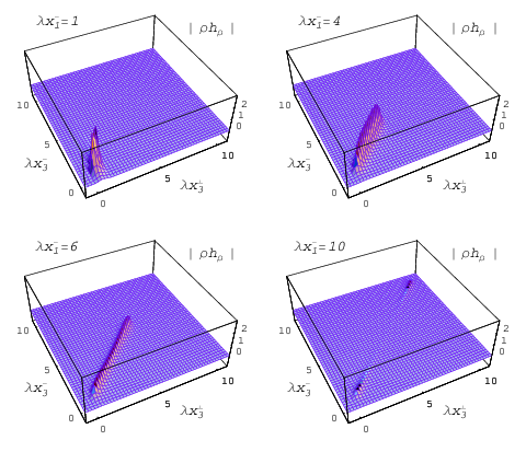
For every choice of , the function is a function of and . Figs. 2 and 3 show examples that illustrate generic features of .
Fig. 2 illustrates how the non-local interaction strength on the LF depends on the position of the point , where particle number 3 is annihilated (created), for a given distance between the two points and , where particles 1 and 2 are created (annihilated). The distances are measured in dimensionless units that result from multiplication of position coordinates by the RGPEP scale parameter . To obtain the Hamiltonian corresponding to , the density whose modulus times is shown in Fig. 2, multiplied by the factors present in Eq. (46) to obtain , is integrated with the product of three effective fields using , see Eq. (3.1).
For the purpose of drawing, Fig. 2 is artificially modified in so far that the infinitesimal parameter is set to 1/5. This substitution causes that the rise of the modulus of due to the square of crossing 0 in denominator is limited to , instead of reaching . The artificial modification preserves generic features of . Namely: a) pointwise decreases with distance between and , b) it quickly vanishes outside the region where is near a straight line connecting with on the LF, and c) it is notably spread toward the end-points when exceeds 4. The number 4 results from the factor in Eq. (47). This factor is varying slowly until exceeds the inverse of maximal value of , which is 16. Thus, when exceeds 4, the density begins to be suppressed in the middle between and . When increases far above 4, the interaction density favors near or , being squeezed in the middle between and .
Fig. 2 illustrates the feature that must lie near a line connecting and on the LF in the cases where . Fig. 3 shows that the same happens in other cases, by providing examples for different orientations of on the LF. Again, is set to in order to avoid infinite values on the line connecting points and , which is the same trick of convenience in drawing that was used earlier in Fig. 2 and is further explained below.

Both Figs. 2 and 3 display partly jagged shapes of the drawn functions, which requires explanation. For this purpose, consider the function
| (49) |
in the vicinity of . Fig. 4 displays the modulus and real part of this function for .

Since Figs. 2 and 3 are drawn using a crude, uniform mesh of points for arguments and a uniform trapezoidal interpolation for shading of the function image, it happens from time to time that the mesh selects an argument point a bit away from a narrow peak (forming a wall of a priori infinite height) in the plotted function. The selected argument produces a small value of the function. When such small value is crudely connected with large values at neighboring points, a somewhat jagged shape is obtained. When the mesh spacing is decreased, drawings become smooth. However, the files with a small mesh spacing have a prohibitive size. Figs. 1, 2, and 3 are provided as a result of a compromise between precision of rendering and size of the figure files. The compromise is made in such a way that in every case the key feature to be displayed and discussed is not altered in any significant way.
3.3 Non-locality for
In attempts to understand mass generation in a relativistic theory of particles, such as attempts to solve QCD for quark and gluon wave functions of hadrons in the Minkowski space or attempts to resolve the strong interaction structure of photons that results in mixing of photons with -mesons, one is faced with a challenge of understanding dynamics of binding of effective constituents of some mass . In QCD, the effective constituent mass that dominates the mechanism of binding of lightest quarks appears to be of the order of . The problem of chiral symmetry breaking in QCD and other theories can be rephrased as a question of what are the dominant interaction terms in an effective Hamiltonian of QCD when the decreasing RGPEP parameter becomes comparable with . In any case, unless the parameter is comparable with or smaller than the constituent mass , a large number of constituents may participate in the dynamics described by Hamiltonians evaluated using RGPEP. Therefore, it is of interest to construct and understand the structure of Hamiltonian interaction terms with small , where by small it is meant that is comparable with . This section discusses the non-locality of first-order RGPEP three-particle vertex in this regime.
It is visible in Fig. 1 that the RGPEP momentum-space form factor peaks at , i.e., in the center of a middle bump in Fig. 1. Section 3.1 shows that the two neighboring regions with below 0 and above 1 both contribute the same operator that the region contributes. As decreases, the size of also decreases. The smaller the weaker the interaction that changes the number of effective particles. However, in asymptotically free theories, the effective coupling constant increases when decreases; may partly compensate for the small size of at its peak. The resulting interaction strength may thus be not eliminated entirely when decreases to about . Instead, the strength is located in the domain in momentum space where is maximal. Therefore, for or smaller, given that the three regions of , , and contribute the same operator to the Hamiltonian, it is sufficient to consider the middle region of in Fig. 1, i.e., the region where forms a bump around . In this region, the relative transverse momentum is limited to values not exceeding order , tempered in addition by how much the variable deviates from 1/2.
For a closer inspection of the middle bump region for , consider the form factor
| (50) |
with given in Eq. (33), rewritten as
| (51) |
The exponential in front describes the size of the form factor at its maximum at and , while the remaining factor describes the form factor fall-off away from its maximum. Now,
| (52) |
where the first factor on the right-hand side is not smaller than while the second factor can be small. These two factors can be analyzed in detail in terms of variables
| (53) | |||||
| (54) | |||||
| (55) |
with which
| (56) | |||||
| (57) |
and
| (58) |
For or smaller, the relative momentum of particles 1 and 2 is smaller than and the RGPEP form factor can be very well approximated by Gaussian
| (59) |
Using this approximation in Eq. (37) written in terms of variables and defined in Eqs. (136) to (139), one obtains
| (60) | |||||
Since for or smaller one has and
| (61) |
the function is approximated by
| (62) | |||||
The key observation is that one can introduce a three-vector
| (63) |
and write
| (64) | |||||
so that the non-locality is parameterized in terms of . Details of evaluation of the non-locality are described in Appendix C. Like in Eqs. (43) to (48) for massless particles, one can write
| (65) |

where and
| (66) |
Using , Eq. (C) implies
| (67) |
For (or ), this result matches the massless case of Eq. (47) up to the factor when . In this case, amounts to 1/4.
Non-locality of the interaction vertex for is illustrated in Fig. 5, which should be compared with Fig. 2. For away from the points with , especially at the end-points, the result for shown in Fig. 5 is quite different from the massless case shown in Fig. 2; there is a strong suppression instead of enhancement at the end points. The smaller , i.e., the smaller , the narrower the peak at and lesser exponential suppression of the non-local vertex due to increase of .
In contrast to Fig. 2, Fig. 5 exhibits the feature that the non-local interaction density prefers the position of in the middle of and . This is a characteristic behavior for non-relativistic interactions, i.e., interactions in which relative momentum of interacting particles is smaller than their masses. Interactions of relativistic particles do not have this feature.
Finally, one can observe that the three points , , and must approximately lie on a straight line on the LF. This feature is the same as in Fig. 3 and does not require a separate drawing.
3.4 Non-locality in a non-relativistic theory
There is an analogy with a non-relativistic quantum mechanics that may be helpful in interpretation of the results described in the previous sections. The difficulty of interpretation may be expected because RGPEP is developed in the front form of Hamiltonian dynamics and the non-locality of interaction Hamiltonian densities is obtained on the LF hyper-plane in space-time rather than in space at a single moment of time. Thus, the relativistic RGPEP involves concepts that are general enough for hoping that the method will apply in derivation of wave functions of bound states of partons in theories with asymptotic freedom and infrared slavery or in attempts to understand symmetry breaking and mass generation at high energies. The space-time concepts do not appear quite intuitive from the point of view based on non-relativistic quantum mechanics. The latter only applies when motion of charged particles is characterized by velocities , where is the speed of light and is the fine structure constant . This constant determines the strength of interactions which govern behavior of electrons bound in atoms. Binding of quarks and gluons occurs in space-time as a result of interactions with coupling constants about 100 times greater than in QED and the non-relativistic intuition is not directly applicable. The same difficulty with building a physical picture is faced in all theories of mass generation and related symmetry breaking.
Fortunately, an intuitive picture to think about can be arrived at by comparing RGPEP form factors for small with simple form factors that may be introduced ad hoc in an effective non-relativistic theory. For example, consider interactions that resemble emission and absorption of mesons by nucleons in nuclear physics. Suppose an effective interaction Hamiltonian has the form
| (68) | |||||
where , 2, 3 are standard three-dimensional momentum variables conjugated with standard rectilinear co-ordinates , 2, 3 in space, respectively. Let an arbitrarily chosen form factor be
| (69) |
Suppose that one builds effective fields at the moment using operators (only annihilation operators) and evaluates a non-local Hamiltonian density in space. Instead of Eq. (37), one is led to consider an expression of the form
| (71) | |||||
| (72) |
and obtains
| (73) |
This result has an intuitive interpretation. Particle 3 is annihilated (created) exactly in the middle of positions and where particles 1 and 2 are created (annihilated), respectively. The width of the distribution of distances between points and is . When , the interaction is local. When becomes small, it is greatly delocalized in the sense that the distance between and can be large, but at the same time is always precisely in the middle between and .
The situation is somewhat similar to the one shown in Fig. 5, except that in Fig. 5 one of the directions is on the LF. However, when is small in comparison with masses and is fairly located on the LF between and , one can observe that for all co-ordinates involved and . Therefore, in the non-relativistic case, can be seen as analogous to . This way one recovers the simple non-relativistic interpretation of the LF non-locality. Further discussion is provided in the next section.
3.5 Relationship to a 2-body wave function
Previous section provided an interpretation of the non-local interaction Hamiltonian densities on the LF by analogy that was limited to slow particles. This section provides another intuitive picture that is more precise and not limited to slowly moving bound states. In fact, it can be used in any frame one wishes to use, including the infinite momentum frame (IMF) and the center of mass frame (CMF) alike.
In order to relate the non-locality of an effective Hamiltonian interaction term to a wave function of a 2-body bound state on the LF hyperplane defined by condition , we introduce three species of particles which are annihilated by operators , , and , respectively. The three species are introduced to avoid the need for symmetrization of relevant functions for identical particles. Masses of the three species are assumed all equal in order to match the conditions set in the previous sections.
Consider the matrix element
| (74) |
where denotes the vacuum state that is annihilated by , , and for . The effective quantum fields , , and are defined by Eqs. (19) to (22) for species 1, 2, and 3, respectively. The superscript means differentiation,
| (75) |
The state with , defined as a particle of the third species
| (76) |
can be considered analogous to a bound state of two effective constituents of species 1 and 2 corresponding to scale . Namely, the eigenvalue equation for a bound state with momentum ,
| (77) |
can be rewritten as
| (78) |
The Hamiltonian couples a pair of particles 1 and 2 with a particle 3. Therefore, the eigenvalue equation for the state involves both the 2-particle component of type 1 and 2 and the 1-particle component of type 3. This LF situation resembles the Lee model [16, 17]. The wave function to focus on is the 2-particle component. One can insert the identity in 2-body space,
| (79) |
on the left-hand side of and evaluate the matrix element
| (80) |
The result takes the form
| (81) |
in which the matrix element
appears in the role of a two-body Green’s function for states with LF energy on the LF hyperplane . The matrix element of Eq. (74) plays the role of a vertex function in Eq. (81).
The Hamiltonian from Eq. (34), plainly modified to the case of three species of particles by associating position with species for and keeping the factor 3 in front, can be inserted into Eq. (74), which yields
By comparison with Eq. (37), the following relation is uncovered between the non-local interaction Hamiltonian densities obtained in first-order RGPEP in previous sections and a 2-body vertex function on the LF:
| (84) |
Inverting the Fourier transform, one obtains
| (85) |
Using expressions derived for in previous sections, one obtains in the case
| (86) | |||||
and in the case
| (87) | |||||
where
| (88) |
Irrespective of the values of particle masses, RGPEP scale , and the coupling constant , the vertex function contains the factor which carries its dimension. The vertex function contains as a factor a plane-wave function of the center-of-mass position variable . Particles 1 and 2 contribute equally to because . The remaining factor is a function of relative motion but depends on the total momentum . More precisely, it has a universal property of being a function of two variables: square of and . Taking into account that , the former variable is equal to a square of a four-vector, , and the latter variable is a product of two four-vectors. Both variables are invariant under 7 kinematical LF symmetries.
The generic structure of the vertex function implies that the Soper variable [18] does not properly separate the center-of-mass motion from the relative motion of constituents. Namely, the parameterization and implies , where the relative momentum has . This means that the product is a mixture of and that depends on . and can be arguments of the relative-motion vertex function, but is not allowed to appear in the plane wave that describes the center-of-mass motion with a definite total momentum . The product is a natural variable to complement as an argument of the vertex function even though these variables have different dimensions (see below).
Another reason for the found structure of the vertex function to be of interest is that there exists an analogy between the LF wave function and AdS/CFT descriptions of bound-state form factors, discovered by Brodsky and de Téramond [19]. In that analogy, the effective transverse distance variable plays a key role as an argument of a bound-state wave function. The question concerning -dependent non-local LF interaction Hamiltonian densities is whether their RGPEP evolution can be understood as dependence on a 5th dimension [20] in the context of duality [21, 22, 23] and whether this dependence can explain the shape of wave functions found by Brodsky and de Téramond. They interpret the analogy between AdS/CFT duality and AdS/QCD picture of hadrons in LF formulation without any need for considering the argument and scale .
The issue of different dimensions of and is resolved in the large- case, i.e., and Eq. (86), by multiplication of by . In the small- case, i.e., and Eq. (87), the same issue is resolved by dividing by the sum of masses of the interacting constituents. The ratio of to the masses becomes a dimensionless parameter.
It is worth noting that the relativistic Eq. (87) predicts in the CMS a small difference between how and enter the vertex function. Namely, for , the ratio becomes and in the CMS equals mass, say , of the state under consideration (consider the Lee model [16]), while when . So, in Eq. (87) becomes , or , where denotes binding energy. This is how the LF vertex function keeps track of the mass defect due to binding. This result requires better understanding than the one offered here. On the other hand, the same Eq. (87) can be used in any frame, including the IMF, where one sees how the interaction vertex or wave function get squeezed due to motion. This is a relativistic squeezing in a quantum theory, not classical.
Finally, it also seems worth mentioning that the relationship identified here between non-local LF interaction vertices and bound-state vertex functions may become helpful in calculating observables such as form factors. The suggestion is based on the fact that the function defined in Eq. (37) gives the same interaction Hamiltonian in Eq. (3.1) that is also obtained in Eq. (25) using defined in Eq. (26). Suppose that the old-fashioned perturbation theory for form factors [24] can be developed using non-local interaction Hamiltonians of the type defined in Eq. (25) with non-locality of the type defined in Eq. (26). Feynman rules with non-local vertices could then suggest how to incorporate all diagrams that count for all kinds of momentum transfers, not only those that have . In the case of local vertex functions [25], it is known what to do when . It is less clear what to do for bound-state vertices that involve non-trivial vertex functions. Therefore, it seems worth checking if the non-local interaction Hamiltonian densities obtained in first-order RGPEP lead to unique answers.
4 Conclusion
Renormalized Hamiltonian densities on the LF hyperplane in space-time contain interaction terms that are non-local. The non-locality is certainly intriguing and needs to be studied for many reasons as a feature of basic interactions. This article makes only a first step in this direction. In particular, we calculate the non-locality in first-order of a perturbative expansion in powers of an effective coupling constant using RGPEP. This is done for terms that originate from a product of three fields. Such terms include coupling of fermions to gauge bosons, coupling of fermions to Yukawa particles, and coupling of non-Abelian gauge bosons with themselves. But the leading non-locality is common to all these cases and can be calculated using scalar fields. The result is that the non-local interaction density has a generic form as a function of the space-time positions of effective particles that are created and annihilated by the interaction. This form can be understood in terms of a vertex function for a two-body bound state.
The characteristic dependence of the vertex function on and , where denotes the bound-state total momentum and denotes the relative position of its two constituents, implies a characteristic dependence of the non-local Hamiltonian density on the position of an annihilated (created) particle relatively to the positions and of created (annihilated) particles in a three-particle vertex. Namely, is distributed near a straight line connecting with on the LF. Figs. 1 to 5 illustrate the shapes of the calculated distributions.
All examples studied here were obtained for all particles having the same mass. For different masses, the results will be numerically different and of more interest from the point of view of application. However, there is no reason to expect a major alteration in the method and results beyond numerical changes. Nevertheless, such changes will be significant in practice.
Another need for generalization concerns interactions that originate from products of more than three fields in one vertex. RGPEP provides a set of general rules for how to calculate non-local interaction densities in such cases order-by-order in perturbation theory. It is not excluded that the terms identified using RGPEP in perturbation theory will lead to a selection of dominant terms for which a non-perturbative evolution can be derived on a computer.
A general speculation is in order concerning the role of non-local interactions in formation of strings of quantum gluons. Imagine that an effective gluon splits non-locally into two along a line as required by the LF non-locality of a Hamiltonian interaction term. Then, each of the two gluons interacts with neighboring gluons. It was argued before using analogy with RGPEP results for heavy quarkonia [26] that gluons of small may attract each other in color singlets by potentials that resemble harmonic oscillator. In this context, the non-local splitting of gluons can be seen as a candidate for dynamical generation of quantum strings in which interactions between neighboring gluons in space are so strong that the string energy grows only linearly with its length, the effective gluon mass at scale providing a unit of energy per unit of length order .
Appendix A Connection of Eqs. (3.1) and (37) with Eqs. (25) and (26)
Details of the connection of interest are provided here for completeness. The connection involves several steps. Each of them involves manipulation of several variables. Understanding the connection requires tracing of these steps. These steps also exhibit an analogy between the momentum labeling of creation and annihilation operators in RGPEP and the parameters in the range between 0 and 1 that appear in old-fashioned perturbation theory for scattering processes in the IMF [27], or parameters in the same range from 0 to 1 that appear in -ordered Feynman rules for calculating scattering amplitudes [14].
Creation and annihilation operators in the interaction Hamiltonian in Eq. (34) stand in normal order and inserting a sign of normal ordering does not change anything. Two terms, both with integration over , can be changed to one term with integration over from to , rendering the result that in Eq. (3.1) equals
| (89) | |||||
One can use defined in Eq. (37) to introduce
| (90) |
and write
where
| (92) | |||||
| (93) | |||||
| (94) |
The function in Eq. (A), defined by Eq. (92), should be the same as the function in Eq. (25), defined by Eq. (26), i.e.,
| (95) | |||||
In order to exhibit equivalence of in Eq. (95) and in Eq. (92), we change integration variables in Eq. (95) according to Eqs. (31) and (32), from and to , and ,
| (96) | |||||
| (97) |
rename to , and obtain
| (98) | |||||
| (99) |
with given by Eqs. (17) and (18). Change of the variable to and integration over yields
| (101) |
which is to be compared with Eq. (92) for using
| (102) | |||||
| (104) |
Note that Eqs. (101) and (92) look similar in terms of integrations and functions they involve. For example, both involve the same integration over and the functions and coincide after replacement of and by and , respectively. However, the two expressions as a whole differ by a factor of 3 in front. The integration over ranges from 0 to 1 while integration over ranges from to . This difference is analogous to the difference between parameters [27] or parameters [14] that range from 0 to 1 ( and were mentioned at the beginning of this Appendix) and the usual momentum variables that range from to . The form factor appears defined in terms of particle momenta differently in both cases. In order to see how these differences conspire to produce the same result, we first evaluate in Eq. (101).
We divide the range of integration over in Eq. (101) into three ranges; one from to 0, shortly called 1, one from 0 to 1, called 2, and one from 1 to , called 3. In each of these 3 regions, we change variables of integration from and to new variables and demonstrate that the resulting expression coincides with 1/3 of in Eq. (92).
| (105) |
where . Using Eqs. (102) to (104),
| (106) |
Thus, for all particles in the interaction term having the same mass ,
| (107) | |||||
The resulting four-vector products read
| (108) | |||||
| (109) | |||||
| (110) |
and the result is that
| (112) | |||||
| (113) |
should match the corresponding expression in Eq. (92), repeated here for the readers’ convenience,
| (115) | |||||
| (116) |
The 0 to 1 part of integration over in Eq. (112) matches exactly 1/3 of Eq. (115). The question is how to see the matching of the remaining 2/3 with parts of integration over from to 0 and from 1 to .
There are two main regions of integration variables, and . Focus on the region . Split integration over into three ranges; range 1 from to 0, range 2 from 0 to 1, and range 3 from 1 to . In the region 2, results match. Consider region 1. For , one has , which means the particle 1 is annihilated, not created, particle 2 is created, and particle 3 is always annihilated for .
So, for , change variables treating as a total momentum (created, with a negative component) composed of and (both annihilated, with positive components). This means
| (117) |
and
| (118) | |||||
| (120) |
The required change of variables is
| (121) | |||||
| (122) |
With this change of variables ( here but it is kept as ),
| (123) | |||||
| (124) |
which is the expected function of and . So, after the change of variables, the region 1 with contributes
| (127) |
Change notation ,
keeping , so that
| (129) |
Then,
where
| (131) |
Changing variable to ,
| (133) | |||||
| (134) |
This result should be compared with 1/3 of given in Eq. (115).
This comparison shows that initial integration range over and thus particles 1 and 2 created and particle 3 annihilated in , corresponds to integration over and thus particles 1 and 3 annihilated and particle 2 created in . When both signs of are included in the integration, the result must be
| (135) |
The next observation is that the integration over and in the Hamiltonian includes only the symmetric part of the functions in Eqs. (25) and (A). Therefore, Eq. (135) completes the explanation of how the integration over range 1 produces 1/3 of the interaction Hamiltonian.
Since the integration in range 3 can be transformed in the same way, the only difference being that for the particle 1 and particle 2 are changed in their roles with respect to particle 3, it follows that the integration over in range 3 produces the remaining 1/3 of the Hamiltonian. Hence, the connection of Eqs. (3.1) and (37) with Eqs. (25) and (26) is established, and both ways of writing the non-local interaction Hamiltonian that results from first-order RGPEP, are equivalent.
Appendix B Integrals involved in non-locality for
In terms of variables
| (136) | |||||
| (137) |
which imply
| (138) | |||||
| (139) |
Eq. (42) reads
| (140) | |||||
Integration over renders
| (141) |
and subsequent integration over gives
| (142) | |||||
Integration over requires regularization. By inserting under the integral and assuming that , one obtains
| (143) | |||||
Hence, the function defined in Eq. (43) is given by Eq. (44).
Appendix C Integrals involved in non-locality for
Introducing a dimensionless three-vectors , where is defined in Eq. (63), and , where is defined in Eqs. (53) and (54), one obtains the function defined in Eq. (64) in the form
| (144) | |||||
Using , one can perform integration over , obtaining
| (145) | |||||
To integrate over , can be written in the form
| (146) | |||||
Then, can be written in terms of two mutually orthogonal transverse vectors, and , as
| (147) |
The auxiliary parameter has nothing to do with introduced earlier. The integral over becomes
| (148) | |||||
| (149) |
The remaining integral over , using , gives
| (150) | |||||
| (151) |
The entire integral is then
| (152) | |||||
The remaining integral over , after the same regularization by factor that was introduced in Appendix B, produces
| (153) | |||||
Using dimensionless variables and , one can write
| (154) |
Since must lie along , so that , one gets
| (155) |
Thus, the approximate result for , where , is
| (156) | |||||
Writing
| (157) |
one arrives at
which results in Eq. (67).
References
- [1] P. A. Dirac, Rev. Mod. Phys. 21, 392 (1949).
- [2] J. B. Kogut, L. Susskind, Phys. Rept. 8, 75 (1973).
- [3] P. P. Srivastava, S. J. Brodsky, Phys. Rev. D 66, 045019 (2002).
- [4] K. G. Wilson et al., Phys. Rev. D 49 6720 (1994).
- [5] S. D. Głazek, Acta Phys. Polon. B 29, 1979 (1998).
- [6] D. J. Gross, F. Wilczek, Phys. Rev. Lett. 30, 1343 (1973).
- [7] H. D. Politzer, Phys. Rev. Lett. 30, 1346 (1973).
- [8] S. D. Głazek, Phys. Rev. D 63, 116006 (2001).
- [9] M. A. Shifman, A.I. Vainshtein, V. I. Zakharov, Nucl. Phys. B 147, 448 (1979).
- [10] K. G. Wilson, Phys. Rev. 140, B445 (1965).
- [11] S. Głazek, J. Młynik, Phys. Rev. D 74, 105015 (2006).
- [12] R. J. Perry, K. G. Wilson, Nucl. Phys. B 403, 587 (1993).
- [13] S.-J. Chang, R. G. Root, T.-M. Yan, Phys. Rev. D 7, 1133 (1973).
- [14] S.-J. Chang, T.-M. Yan, Phys. Rev. D 7, 1147 (1973).
- [15] R. P. Feynman, Phys. Rev. 84, 108 (1951).
- [16] T. D. Lee, Phys. Rev. 95, 1329 (1954).
- [17] T. Masłowski, M. Wiȩckowski, Phys. Rev. D 57, 4976 (1998).
- [18] D. E. Soper, Phys. Rev. D 15, 1141 (1977).
- [19] G. F. de Téramond, S. J. Brodsky, Phys. Rev. Lett. 102, 081601 (2009).
- [20] S. D. Głazek, Acta Phys. Polon. B 39, 3395 (2008).
- [21] A. M. Polyakov, Int. J. Mod. Phys. A 14, 645 (1999); Eq. (39).
- [22] S. S. Gubser, I. R. Klebanov, A. M. Polyakov, Phys. Lett. B 428, 105 (1998).
- [23] O. Aharony et al., Phys. Rept. 323, 183 (2000).
- [24] J. F. Gunion, S. J. Brodsky, R. Blankenbecler Phys. Rev. D 8, 287 (1973).
- [25] S. D. Głazek, M. Sawicki, Phys. Rev. D 41, 2563 (1990).
- [26] Ref. [11], Sec. VI.
- [27] S. Weinberg, Phys. Rev. 150, 1313 (1966).