RNA-RNA binding is an important phenomenon observed in various classes of non-coding RNAs and plays a crucial role in a number of regulation processes. Regulatory antisense RNAs control gene expression by prohibiting the translation of a target mRNA through establishing stable base pairing interactions. Examples include the regulation of translation in both: prokaryotes [1] and eukaryotes [2, 3], the targeting of chemical modifications [4], insertion editing [5], and transcriptional control [6]. More and more evidence suggests, that RNA-RNA interactions also play a role for the functionality of long mRNA—like ncRNAs [7]. A common theme in many RNA classes, including miRNAs, snRNAs, gRNAs, snoRNAs, and in particular many of the procaryotic small RNAs, is the formation of RNA-RNA interaction structures that are much more complex than simple complementary sense-antisense interactions. The interaction between two RNAs is governed by the same physical principles that determine RNA folding: the formation of specific base pairs patterns whose energy is largely determined by base pair stacking and loop strains. As a result, secondary structures are an appropriate level of description to quantitatively understand the thermodynamics of RNA-RNA binding.

Alkan et al. [8] proved that the RNA-RNA interaction prediction (RIP) problem is in its general form NP-complete. Nevertheless, we are facing increasing demand for efficient computational methods for RIP. By restricting the space of allowed configurations, polynomial-time algorithms on secondary structure level have been derived. Pervouchine [9] and Alkan et al. [8] proposed MFE folding algorithms for predicting the joint structure of two interacting RNA molecules. In this model, “joint structure” means that the intramolecular structures of each partner are pseudoknot-free, that the intermolecular binding pairs are noncrossing, and that there is no so-called “zig-zag” configuration, see Fig. 1. The optimal joint structure can be computed in $O(N^{6})$ time and $O(N^{4})$ space by means of dynamic programming [8, 9, 12, 13]. Extensions involving the partition function were proposed by Chitsaz et al. (piRNA) [13] and Huang et al. (rip) [14].

In contrast to the situation for RNA secondary structures [15, 16], much less is known about joint structures. Only joint structures of arc-length greater than or equal to two have been studied in [17]. However, the biochemistry of nucleotide-pairings, favors parallel stacking of bonds due to entropy and the minimum length of intramolecular bonds of four. Unfortunately, the biophysically relevant class of canonical joint structures with arc-length $\geq 4$, is not governed by the framework in [17].

In this paper, we introduce the general framework dealing with $\sigma$-canonical joint structures having arc-length $\geq\sigma+2$. In particular, our results apply to the class of canonical joint structures having arc-length $\geq 4$. Our results are relevant for the design and analysis of RIP folding algorithms and show that the numbers of $\sigma$-canonical joint structures with arc-length $\geq\sigma+2$ exhibit surprisingly small exponential growth rates.

This paper is organized as follows: in Section 2 we introduce joint structures along the lines of [12] and in Section 3 we compute, along the lines of [18], the generating function of refined shapes via symbolic enumeration. In Section 4 we show how to inflate refined shapes into joint structures and derive the generating function of joint structures. Section 5 presents the singularity analysis and asymptotic formulas. We finally integrate our results in Section 6.

Let us begin by discussing some basic results of [15, 16, 19]. Let $f(n)$ denote the number of all noncrossing matchings of $n$ arcs having the generating function ${\bf F}(z)=\sum f(n)\,z^{n}$. Recursions for $f(n)$ allow us to derive $z\,{\bf F}(z)^{2}-{\bf F}(z)+1=0$, that is we have

Let $\mathcal{T}_{\sigma}^{[\lambda]}$ denote the combinatorial class of $\sigma$-canonical secondary structures having arc-length $\geq\lambda$ and $T_{\sigma}^{[\lambda]}(n)$ denote the number of all $\sigma$-canonical secondary structures over $n$ vertices having arc-length $\geq\lambda$ and

Theorem 1 implies that for any specified $\lambda$ and $\sigma$, ${\bf T}^{[\lambda]}_{\sigma}(z)$ is algebraic over the rational function field $\mathbb{C}(z)$, since ${\bf F}(z)$ is algebraic and $v_{\lambda}(z),u_{\sigma}(z)$ are both rational functions.

Given two RNA sequences $R=(R_{i})_{1}^{n}$ and $S=(S_{j})_{1}^{m}$ with $n$ and $m$ vertices, we index the vertices such that $R_{1}$ is the $5^{\prime}$ end of $R$ and $S_{1}$ is the $3^{\prime}$ end of $S$. The intramolecular base pair can be represented by an arc (interior), with its two endpoints contained in either $R$ or $S$. Similarly, the extramolecular base pair can be represented by an arc (exterior) with one of its endpoints contained in $R$ and the other in $S$. When representing arc-configurations, we draw all $R$-arcs in the upper-halfplane and all $S$-arcs in the lower-halfplane, see Fig. 2, (A).

We refer to the subgraph induced by $\{R_{i},\ldots,R_{j}\}$ by $R[i,j]$. The subgraph $R[i,j]$ ($S[i^{\prime},j^{\prime}]$) is called secondary segment if there is no exterior arc $R_{k}S_{k^{\prime}}$ such that $i\leq k\leq j$ ($i^{\prime}\leq k^{\prime}\leq j^{\prime}$), see Fig. 2, (A). An interior arc $R_{i}R_{j}$ is an $R$-ancestor of the exterior arc $R_{k}S_{k^{\prime}}$ if $i<k<j$. Analogously, $S_{i^{\prime}}S_{j^{\prime}}$ is an $S$-ancestor of $R_{k}S_{k^{\prime}}$ if $i^{\prime}<k^{\prime}<j^{\prime}$. We also refer to $R_{k}S_{k^{\prime}}$ as a descendant of $R_{i}R_{j}$ and $S_{i^{\prime}}S_{j^{\prime}}$ in this situation, see Fig. 2, (A). Furthermore, we call $R_{i}R_{j}$ and $S_{i^{\prime}}S_{j^{\prime}}$ dependent if they have a common descendant and independent, otherwise. Let $R_{i}R_{j}$ and $S_{i^{\prime}}S_{j^{\prime}}$ be two dependent interior arcs. Then $R_{i}R_{j}$ subsumes $S_{i^{\prime}}S_{j^{\prime}}$, or $S_{i^{\prime}}S_{j^{\prime}}$ is subsumed in $R_{i}R_{j}$, if for any $R_{k}S_{k^{\prime}}\in I$, $i^{\prime}<k^{\prime}<j^{\prime}$ implies $i<k<j$, that is, the set of descendants of $S_{i^{\prime}}S_{j^{\prime}}$ is contained in the set of descendants of $R_{i}R_{j}$, see Fig. 2, (A). A zigzag is a subgraph containing two dependent interior arcs $R_{i}R_{j}$ and $S_{i^{\prime}}S_{j^{\prime}}$ neither one subsuming the other, see Fig. 2, (B).

A joint structure [9, 8, 13, 12] $J(R,S,I)$, see Fig. 2, (A), is a graph such that

1. (1)

   $R$, $S$ are secondary structures (each nucleotide being paired with at most one other nucleotide via hydrogen bonds, without internal pseudoknots);

2. (2)

   $I$ is a set of exterior arcs without external pseudoknots, i.e., if $R_{i}S_{j}$, $R_{i^{\prime}}S_{j^{\prime}}\in I$ then $i<i^{\prime}$ implies $j<j^{\prime}$;

3. (3)

   $J(R,S,I)$ contains no zig-zags.

We next specify some notations

• •

  an interior arc (or simply arc) of length $\lambda$ is an arc $R_{i}R_{j}$ ($S_{i^{\prime}}S_{j^{\prime}}$) where $j-i=\lambda$ ($j^{\prime}-i^{\prime}=\lambda$),

• •

  an interior stack (or simply stack) of length $\sigma$ is a maximal sequence of “parallel” interior arcs,

  	$\displaystyle(R_{i}R_{j},R_{i+1}R_{j-1},\ldots,R_{i+\sigma-1}R_{j-\sigma+1})$	or
  	$\displaystyle(S_{i}S_{j},S_{i+1}S_{j-1},\ldots,S_{i+\sigma-1}S_{j-\sigma+1}),$

• •

  an exterior stack of length $\tau$ is a maximal sequence of “parallel” exterior arcs,

  $$(R_{i}S_{i^{\prime}},R_{i+1}S_{i^{\prime}+1},\ldots,R_{i+\tau-1}S_{i^{\prime}+\tau-1}).$$

A $\sigma$-canonical joint structure is a joint structure with stack-length $\geq\sigma$. In Fig. 2, (A), we give an example of $2$-canonical joint structure with arc-length $\geq 4$.

Let the block $J_{i,j;i^{\prime},j^{\prime}}$ denote the subgraph of a joint structure $J(R,S,I)$ induced by a pair of subsequences $\{R_{i},R_{i+1},\ldots,R_{j}\}$ and $\{S_{i^{\prime}},S_{i^{\prime}+1},\ldots,S_{j^{\prime}}\}$. Given a joint structure $J(R,S,I)$, a tight structure of $J(R,S,I)$ is the minimal block $J_{i,j;i^{\prime},j^{\prime}}$ containing all the $R$-ancestors and $S$-ancestors of any exterior arc in $J_{i,j;i^{\prime},j^{\prime}}$ and all the descendants of any interior arc in $J_{i,j;i^{\prime},j^{\prime}}$. In the following, a tight structure is denoted by $J^{T}_{i,j;i^{\prime},j^{\prime}}$. In particular, we denote the joint structure $J(R,S,I)$ by $J^{T}(R,S,I)$ if $J(R,S,I)$ is a tight structure of itself. For any joint structure, there are only four types of tight structures $J^{T}_{i,j;i^{\prime},j^{\prime}}$, that is $\{\circ,\triangledown,\vartriangle,\square\}$, denoted by $J^{\{\circ,\triangledown,\vartriangle,\square\}}_{i,j;i^{\prime},j^{\prime}}$, respectively, see Fig. 3.

The key function of tight structures is that they are the building blocks for the decomposition of joint structures.

In Fig. 4 we illustrate the decomposition of a joint structure.

A shape [17] is a joint structure containing no secondary segments in which each interior stack and each exterior stack have length exactly one. We follow the ideas in [18] and obtain the generating function of joint structures via inflation of refined (colored) shapes. Refined shapes are obtained by distinguishing two classes of exterior shape-arcs. Each distinguished class requires its specific inflation-procedure (see Theorem 2). Let us have a closer look at two particular classes of exterior arcs:

• •

  Class $\mathbf{A}_{1}$: the class of arc-pairs $(\alpha,\beta)$ where $\alpha$ is an exterior arc with the unique interior $2$-arc $\beta$ as its ancestor.

• •

  Class $\mathbf{A}_{2}$: the class of arc-triples $(\alpha,\beta,\gamma)$ where $\alpha$ is an exterior arc with interior $2$-arcs $\beta$ and $\gamma$ as ancestors.

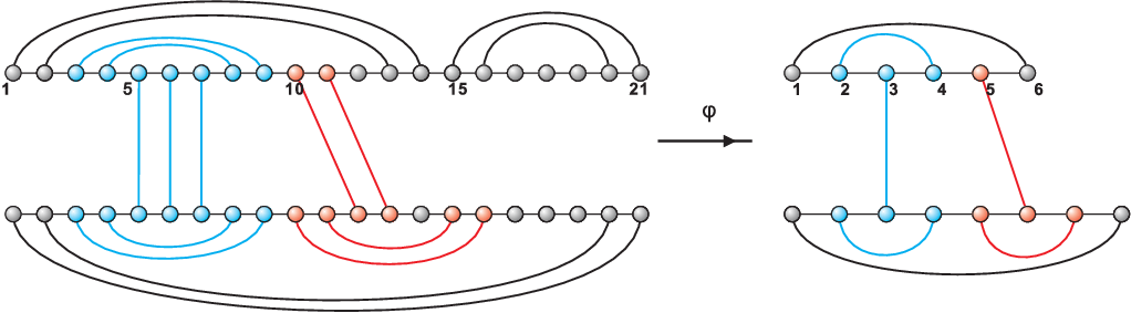
Let $\mathcal{G}$ denote the combinatorial class of shapes. Given a joint structure, we can obtain its shape by first removing all secondary segments and second collapsing any stack into a single arc. That is, we have a map $\varphi\colon{\mathcal{J}}\rightarrow{\mathcal{G}}$. In Fig. 5, we illustrate how a joint structure is projected into its refined shape. The resulting shape exhibits elements in class ${\bf A}_{1}$ as well as class ${\bf A}_{2}$.

Let $G(t,h,a_{1},a_{2})$ denote the number of shapes having total $t$ interior arcs and $h$ exterior arcs containing $a_{1}$ elements of class ${\bf A}_{1}$ and $a_{2}$ elements of class ${\bf A}_{2}$ and

We shall proceed by revisiting the notions of tight shapes, double tight shapes, interaction segments, closed shapes and right closed shapes [12]:

• •

  a tight shape is tight as a structure. Let $\mathcal{G}^{T}$ denote the class of tight shapes and $G^{T}(t,h,a_{1},a_{2})$ denote the number of tight shapes having total $t$ interior arcs and $h$ exterior arcs containing $a_{1}$ elements of class ${\bf A}_{1}$ and $a_{2}$ elements of class ${\bf A}_{2}$,

  $${\bf G}^{T}(x,z,u,v)=\sum G^{T}(t,h,a_{1},a_{2})\,x^{t}z^{h}u^{a_{1}}v^{a_{2}}.$$

  Any tight shape, comes as exactly one of the four types $\{\circ,\triangledown,\vartriangle,\square\}$. The corresponding classes and generating functions are defined accordingly, $\mathcal{G}^{\{\circ,\triangledown,\vartriangle,\square\}}$ and ${\bf G}^{\{\circ,\triangledown,\vartriangle,\square\}}(x,z,u,v)$ respectively,

• •

  a double tight shape is a shape whose leftmost and rightmost blocks are tight structures. Let $\mathcal{G}^{DT}$ denote the class of double tight shapes and $G^{DT}(t,h,a_{1},a_{2})$ denote the number of double tight shapes having total $t$ interior arcs and $h$ exterior arcs containing $a_{1}$ elements of class ${\bf A}_{1}$ and $a_{2}$ elements of class ${\bf A}_{2}$,

  $${\bf G}^{DT}(x,z,u,v)=\sum G^{DT}(t,h,a_{1},a_{2})\,x^{t}z^{h}u^{a_{1}}v^{a_{2}},$$

• •

  a closed shape is a tight shape of type $\{\triangledown,\vartriangle,\square\}$. Let $\mathcal{G}^{C}$ denote the class of closed shapes and $G^{C}(t,h,a_{1},a_{2})$ denote the number of closed shapes having total $t$ interior arcs and $h$ exterior arcs containing $a_{1}$ elements of class ${\bf A}_{1}$ and $a_{2}$ elements of class ${\bf A}_{2}$,

  $${\bf G}^{C}(x,z,u,v)=\sum G^{C}(t,h,a_{1},a_{2})\,x^{t}z^{h}u^{a_{1}}v^{a_{2}},$$

• •

  a right closed shape is a shape whose rightmost block is a closed shape rather than an exterior arc. Let $\mathcal{G}^{RC}$ denote the class of right closed shapes and $G^{RC}(t,h,a_{1},a_{2})$ denote the number of right close shapes having total $t$ interior arcs and $h$ exterior arcs containing $a_{1}$ elements of class ${\bf A}_{1}$ and $a_{2}$ elements of class ${\bf A}_{2}$,

  $${\bf G}^{RC}(x,z,u,v)=\sum G^{RC}(t,h,a_{1},a_{2})\,x^{t}z^{h}u^{a_{1}}v^{a_{2}},$$

• •

  in a shape, an interaction segment is an empty structure or a tight structure of type $\circ$ (an exterior arc). We denote the class of interaction segment by $\mathcal{I}$ and the associated generating function by ${\bf I}(x,z,u,v)$. Obviously, ${\bf I}(x,z,u,v)=1+z$.

Let $\mathcal{H}_{\sigma}$ denote the class of $\sigma$-canonical joint structures with arc-length $\geq\sigma+2$. Let $H_{\sigma}(s)$ denote the number of joint structures in $\mathcal{H}_{\sigma}$ with total $s$ vertices having the generating function

We are now in position to compute the generating function $\mathbf{H}_{\sigma}(x)$. Our strategy is inflating the shapes with specific inflation on specific exterior arcs.

In this section, we derive simple formulas for the number of joint structures in the limit of long sequences.

References

• [1] F. Narberhaus, J. Vogel, Sensory and regulatory RNAs in prokaryotes: A new german research focus, RNA Biol. 4 (2007) 160–164.
• [2] M.T. McManus, P.A. Sharp, Gene silencing in mammals by small interfering RNAs, Nature Reviews 3 (2002) 737–747.
• [3] D. Banerjee, F. Slack, Control of developmental timing by small temporal RNAs: a paradigm for RNA-mediated regulation of gene expression, Bioessays 24 (2002) 119–129.
• [4] J.P. Bachellerie, J. Cavaillé, A. Hüttenhofer, The expanding snoRNA world, Biochimie 84 (2002) 775–790.
• [5] R. Benne, RNA editing in trypanosomes. the use of guide RNAs, Mol. Biol. Rep. 16 (1992) 217–227.
• [6] J.F. Kugel, J.A. Goodrich, An RNA transcriptional regulator templates its own regulatory RNA, Nat. Struct. Mol. Biol. 3 (2007) 89–90.
• [7] B. Hekimoglu, L. Ringrose, Non-coding RNAs in polycomb/trithorax regulation, RNA Biol. 6 (2009) 129–137.
• [8] C. Alkan, E. Karakoc, J.H. Nadeau, S.C. Sahinalp, K. Zhang, RNA-RNA interaction prediction and antisense RNA target search, J. Comput. Biol. 13 (2006) 267–282.
• [9] D.D. Pervouchine, IRIS: Intermolecular RNA interaction search, Proc. Genome Informatics 15 (2004) 92–101.
• [10] I. Lebars, P. Legrand, A. Aimé, N. Pinaud, S. Fribourg, C. Di Primo, Exploring TAR-RNA aptamer loop-loop interaction by X-ray crystallography, UV spectroscopy and surface plasmon resonance, Nucleic Acids Res. 36 (2008) 7146–7156.
• [11] R. Salari, R. Backofen, S.C. Sahinalp, Fast prediction of RNA-RNA interaction, Algorithms Mol Biol (2010) doi:10.1186/1748-7188-5-5.
• [12] F.W.D. Huang, J. Qin, P.F. Stadler, C.M. Reidys, Partition function and base pairing probabilities for RNA-RNA interaction prediction, Bioinformatics 25 (2009) 2646–2654.
• [13] H. Chitsaz, R. Salari, S.C. Sahinalp, R. Backofen, A partition function algorithm for interacting nucleic acid strands, Bioinformatics 25 (2009) i365–i373.
• [14] F.W.D. Huang, J. Qin, P.F. Stadler, C.M. Reidys, Target prediction and a statistical sampling algorithm for RNA-RNA interaction, Bioinformatics 26 (2010) 175–181.
• [15] M.S. Waterman, T.F. Smith, RNA secondary structure: A complete mathematical analysis, Math. Biosci 42 (1978) 257–266.
• [16] W.R. Schmitt, M.S. Waterman, Linear trees and RNA secondary structure, Disc. Appl. Math. 51 (1994) 317–323.
• [17] T.J.X. Li, C.M. Reidys, Combinatorics of RNA-RNA interaction, in press arXiv:1006.2924v1.
• [18] C.M. Reidys, R.R. Wang, A.Y.Y. Zhao, Modular, kk-noncrossing diagrams, Electron. J. Combin. (2010).
• [19] E.Y. Jin, C.M. Reidys, Combinatorial design of pseudoknot RNA, Adv. Appl. Math. 42 (2009) 135–151.
• [20] R.P. Stanley, Enumerative Combinatorics, Volume 2, Cambridge Uninversity Press, Cambridge, England, 1999.
• [21] E.C. Titchmarsh, The theory of functions, Oxford Uninversity Press, Oxford UK, 1939.
• [22] I.L. Hofacker, P. Schuster, P.F. Stadler Combinatorics of RNA secondary structures, Discr. Appl. Math. 88 (1998) 207–237.
• [23] P. Flajolet, R. Sedgewick, Analytic combinatorics, Cambridge University Press, 2008.