跳到论文正文
W Papers独立论文阅读器 arXiv:1006.4086 论文正文 计算阅读时间 · 0%
引用这篇论文根据当前论文元数据生成,正式投稿前建议核对。


License: arXiv.org perpetual non-exclusive license
arXiv:1006.4086v2 [math.DS] 24 Mar 2011

The Packing Spectrum for Birkhoff Averages on a self-affine RepellerThanks: The author would like to thank Thomas Jordan and Michał Rams for all their help in preparing this paper. This project was started in the Instytut Matematyczny PAN and I would also like to thank the Institute, especially Feliks Przytycki, for their kind hospitality. I would also like to thank the Engineering and Physical Sciences Research Council and the Conformal Structures and Dynamics network for their financial support. In addition I would like to thank the referee, whose careful reading of this paper has greatly improved the presentation.

Henry WJ Reeve Address: Henry WJ Reeve
Department of Mathematics
The University of Bristol
University Walk
Clifton
Bristol
BS8 1TW
UK.
Email address: henrywjreeve@googlemail.com
Abstract.

We consider the multifractal analysis for Birkhoff averages of continuous potentials on a self-affine Sierpiński sponge. In particular, we give a variational principal for the packing dimension of the level sets. Furthermore, we prove that the packing spectrum is concave and continuous. We give a sufficient condition for the packing spectrum to be real analytic, but show that for general Hölder continuous potentials, this need not be the case. We also give a precise criterion for when the packing spectrum attains the full packing dimension of the repeller. Again, we present an example showing that this is not always the case.

1. Introduction and Statement of Results

Let Λ\Lambda be the repeller of a C1+ϵC^{1+\epsilon} map f:X→Xf:X\rightarrow X. Given some continuous potential φ:Λ→ℝN\varphi:\Lambda\rightarrow\mathbb{R}^{N} and some α∈ℝN\alpha\in\mathbb{R}^{N} we are interested in the set of points in the repeller for which the Birkhoff average converges to α\alpha,

(1.1) Eφ​(α):={x∈Λ:limn→∞1n​∑q=0n−1φ⁡(fq​(x))=α}.E_{\varphi}(\alpha):=\bigg\{x\in\Lambda:\lim_{n\rightarrow\infty}\frac{1}{n}\sum_{q=0}^{n-1}\varphi(f^{q}(x))=\alpha\bigg\}.

We would like to understand how the geometric complexity of Eφ​(α)E_{\varphi}(\alpha) varies as a function of α\alpha. Geometric complexity, here, is to be understood in terms of the dual notions of Hausdorff dimension dimℋ\mbox{dim}_{\mathcal{H}}, defined in terms of minimal coverings, and packing dimension dim𝒫\mbox{dim}_{\mathcal{P}}, defined in terms of maximal packings (see [Ed1, Section 6.2] or [Fa2, Chapter 3]). We refer to α↦dimℋ​Eφ​(α)\alpha\mapsto\mbox{dim}_{\mathcal{H}}E_{\varphi}(\alpha) as the Hausdorff spectrum and α↦dim𝒫​Eφ​(α)\alpha\mapsto\mbox{dim}_{\mathcal{P}}E_{\varphi}(\alpha) as the packing spectrum.

In the conformal setting there is a well known variational principle giving the values for both spectra. To recall this result we require some terminology. Let Λ\Lambda be a repeller for an expanding C1+ϵC^{1+\epsilon} map ff of a smooth manifold XX. We let ℳ⁡(Λ,f)\mathcal{M}(\Lambda,f) denote the set of ff-invariant Borel probability measures supported on Λ\Lambda. Given μ∈ℳ⁡(Λ,f)\mu\in\mathcal{M}(\Lambda,f) we let hμ​(f)h_{\mu}(f) denote the Kolmogorov-Sinai entropy (see [Wa, Section 4.10]) and let λμ​(f):=∫log⁡‖f′‖​𝑑μ\lambda_{\mu}(f):=\int\log||f^{\prime}||d\mu denote the Lyapunov exponent. Given a continuous potential φ:Λ→ℝ\varphi:\Lambda\rightarrow\mathbb{R} we let A⁡(φ):={∫φ​𝑑μ:μ∈ℳ⁡(Λ,f)}A(\varphi):=\{\int\varphi d\mu:\mu\in\mathcal{M}(\Lambda,f)\}. We may now recall the classic result due to Pesin and Weiss [PW1], Fan, Feng and Wu [FFW], Barreira and Saussol [BSa], Feng, Lau and Wu [FLW] and Olsen [Ol1], [Ol3]. See also [JJOP] and [GR] for extensions to classes of non-uniformly hyperbolic functions.

Theorem 1 (Feng, Lau, Wu).

Let Λ\Lambda be the repeller for an expanding C1+ϵC^{1+\epsilon} map f:X→Xf:X\rightarrow X. Suppose that ff is conformal and topologically mixing on Λ\Lambda. Then for all α∈A⁡(φ)\alpha\in A(\varphi) we have

dimℋEφ(α)=dim𝒫Eφ(α)=sup{hμ​(f)λμ​(f):μ∈ℳ(Λ,f),∫φdμ=α}.\displaystyle\mbox{dim}_{\mathcal{H}}E_{\varphi}(\alpha)=\mbox{dim}_{\mathcal{P}}E_{\varphi}(\alpha)=\sup\left\{\frac{h_{\mu}(f)}{\lambda_{\mu}(f)}:\mu\in\mathcal{M}(\Lambda,f),\int\varphi d\mu=\alpha\right\}.

In particular, when ff is conformal and uniformly hyperbolic the Hausdorff and packing spectra coincide. This is a consequence of the fact that the level set Eφ​(α)E_{\varphi}(\alpha) corresponds to a type of statistical convergence, together with the neat relationship between geometric and statistical properties which holds in the conformal setting. By contrast, the packing and Hausdorff dimensions of level sets defined in terms of divergent asymptotic properties may differ (see [BOS] and [Ol3]). Theorem 1 also allows one to deduce various regularity properties of the spectrum ([PW2], [FFW], [BSa], [Ol1]). The spectrum is continuous and when φ\varphi is Hölder continuous it is also real analytic. When the Lyapunov exponent λμ​(f)\lambda_{\mu}(f) is given by a fixed constant, independent of μ∈ℳ⁡(Λ,f)\mu\in\mathcal{M}(\Lambda,f), the spectrum is also concave.

The dimension theory of non-conformal systems, for which there is no simple correspondence between geometric and statistical properties, is much less well understood. For the most part we only have almost all type results, both for the dimension of a repeller [Fa1] and for the dimension of level sets for Birkhoff averages [JS]. One class of non conformal fractals for which we do have deterministic results ([Be], [Ki], [McM], [JR], [BM1], [Ni], [KP]) are the self-affine Sierpiński sponges introduced by Bedford [Be] and McMullen [McM] and generalized by Kenyon and Peres [KP].

Definition 1.1 (Self-affine Sierpiński sponges).

Let 𝕋d:=ℝd/ℤd\mathbb{T}^{d}:=\mathbb{R}^{d}/\mathbb{Z}^{d} denote the dd dimensional torus. Choose natural numbers a1>a2>⋯>ad≥2a_{1}>a_{2}>\cdots>a_{d}\geq 2. Let ff denote the integer valued diagonal map given by

(1.2) (xq)q=1d↦(aq​xq)q=1d​ for ​(xq)q=1d∈𝕋d.(x_{q})_{q=1}^{d}\mapsto(a_{q}x_{q})_{q=1}^{d}\text{ for }(x_{q})_{q=1}^{d}\in\mathbb{T}^{d}.

Given a digit set 𝒟⊆∏q=1d{0,⋯,aq−1}\mathcal{D}\subseteq\prod_{q=1}^{d}\left\{0,\cdots,a_{q}-1\right\} there is a corresponding self-affine repeller Λ\Lambda given by

(1.3) Λ:={(∑ν=1∞iq​(ν)aqν)q=1d:(iq​(ν))q=1d∈𝒟​ for all ​ν∈ℕ}.\Lambda:=\left\{\left(\sum_{\nu=1}^{\infty}\frac{i_{q}(\nu)}{a_{q}^{\nu}}\right)_{q=1}^{d}:(i_{q}(\nu))_{q=1}^{d}\in\mathcal{D}\text{ for all }\nu\in\mathbb{N}\right\}.

A limit set Λ\Lambda defined in this way is referred to as a self-affine Sierpiński sponge. A two dimensional Sierpiński sponge is known as a Bedford-McMullen carpet.

Refer to caption
Figure 1. A representation of a digit set (left) and the corresponding Bedford-McMullen carpet (right).

To state the relevant results concerning self-affine Sierpiński sponges we first introduce some terminology. Given a continuous transformation TT of a metric space XX we let ℳ⁡(X,T)\mathcal{M}(X,T) denote the set of TT-invariant Borel probability measures, and let ℰ⁡(X,T)\mathcal{E}(X,T) denote the set of μ∈ℳ⁡(X,T)\mu\in\mathcal{M}(X,T) which are ergodic.

Given k≤dk\leq d we let πk:𝕋d→𝕋d−(k−1)\pi_{k}:\mathbb{T}^{d}\rightarrow\mathbb{T}^{d-(k-1)} be the projection πk:(xq)q=1d↦(xq)q=kd\pi_{k}:(x_{q})_{q=1}^{d}\mapsto(x_{q})_{q=k}^{d}. We let fk:𝕋d−(q−1)→𝕋d−(q−1)f_{k}:\mathbb{T}^{d-(q-1)}\rightarrow\mathbb{T}^{d-(q-1)} denote the map (xq)q=kd↦(aq​xq)q=kd(x_{q})_{q=k}^{d}\mapsto(a_{q}x_{q})_{q=k}^{d}.

Suppose A⊆ℳ⁡(Λ,f)A\subseteq\mathcal{M}(\Lambda,f). For each k≤dk\leq d we define Hk​(f,A)H^{k}(f,A) by

Hk​(f,A)\displaystyle H^{k}(f,A) :⁣=\displaystyle:= sup{hμ∘πk−1​(fk):μ∈A}.\displaystyle\sup\left\{h_{\mu\circ\pi_{k}^{-1}}(f_{k}):\mu\in A\right\}.

When A=ℳ⁡(Λ,f)A=\mathcal{M}(\Lambda,f) we write Hk​(f,A)=Hk​(f)H^{k}(f,A)=H^{k}(f).

The following result is due to Kenyon and Peres [KP].

Theorem 2 (Kenyon, Peres).

Let Λ\Lambda be a self-affine Sierpiński sponge. Then,

dimℋ​(Λ)\displaystyle\mbox{dim}_{\mathcal{H}}(\Lambda) =\displaystyle= supμ∈ℳ⁡(𝕋d,f){hμ​(f)log⁡a1+∑k=2d(1log⁡ak−1log⁡ak−1)​hμ∘πk−1​(fk)},\displaystyle\sup_{\mu\in\mathcal{M}(\mathbb{T}^{d},f)}\left\{\frac{h_{\mu}(f)}{\log a_{1}}+\sum_{k=2}^{d}\left(\frac{1}{\log a_{k}}-\frac{1}{\log a_{k-1}}\right)h_{\mu\circ\pi_{k}^{-1}}(f_{k})\right\},
dim𝒫​(Λ)\displaystyle\mbox{dim}_{\mathcal{P}}(\Lambda) =\displaystyle= H1​(f)log⁡a1+∑k=2d(1log⁡ak−1log⁡ak−1)​Hk​(f).\displaystyle\frac{H^{1}(f)}{\log a_{1}}+\sum_{k=2}^{d}\left(\frac{1}{\log a_{k}}-\frac{1}{\log a_{k-1}}\right)H^{k}(f).

Bedford [Be] and McMullen [McM] independently determined both the Hausdorff dimension and the upper box dimension in the two dimensional setting. In [KP] Kenyon and Peres extend these results to higher dimensions. It follows from [Fa3, Proposition 3.6] that the formula for upper box dimension also gives an expression for the packing dimension.

The multifractal analysis of Birkhoff averages is closely related to the multifractal analysis of pointiwise dimension. Given an invariant measure ν∈ℳ⁡(Λ,f)\nu\in\mathcal{M}(\Lambda,f) on a self-affine Sierpiński sponge Λ\Lambda the Hausdorff and packing spectrums for pointwise dimension are given by α↦dimℋ​Dν​(α)\alpha\mapsto\mbox{dim}_{\mathcal{H}}D_{\nu}(\alpha) and α↦dim𝒫​Dν​(α)\alpha\mapsto\mbox{dim}_{\mathcal{P}}D_{\nu}(\alpha), respectively, where

(1.4) Dν​(α):={x∈Λ:limr→0log⁡ν⁡(B⁡(x,r))log⁡r=α}.D_{\nu}(\alpha):=\left\{x\in\Lambda:\lim_{r\rightarrow 0}\frac{\log\nu(B(x,r))}{\log r}=\alpha\right\}.

In [Ki] King determined the Hausdorff spectrum for Bernoulli measures on a Bedford-McMullen carpet with strong separation conditions. Olsen extended King’s result to Bernoulli measures on dd dimensional self-affine Sierpiński sponge [Ol4]. The Hausdorff spectrum for Gibbs measures was determined by Barral and Mensi [BM2] for Bedford-McMullen carpets, and by Barral and Feng [BF] for a dd dimensional self-affine Sierpiński sponge. In [JR] Jordan and Rams gave the Hausdorff spectrum for Bernoulli measures on a Bedford-McMullen carpet without the strong separation conditions required in [Ki], [Ol4], [BM2] and [BF]. In contrast almost nothing is known about the packing spectrum for pointwise dimension on a self-affine Sierpiński sponge. In this paper we determine α↦dim𝒫​Dν​(α)\alpha\mapsto\mbox{dim}_{\mathcal{P}}D_{\nu}(\alpha) for a very limited class of Bernoulli measures ν\nu on self-affine Sierpiński sponges with strong separation conditions. We also give an example disproving a conjecture of Olsen [Ol4, Conjecture 4.1.7] (see Section 7). However, the main focus for this article is the packing spectrum for Birkhoff averages.

The first result concerning the multifractal analysis of Birkhoff averages for self-affine Sierpiński sponges is due to Nielsen [Ni]. Suppose Λ\Lambda is a self-affine Sierpiński sponge. For x∈Λx\in\Lambda we let

Γ⁡(x):={((iq​(ν))q=1d)ν∈ℕ:x=(∑ν=1∞iq​(ν)aqν)q=1d}.\Gamma(x):=\left\{((i_{q}(\nu))_{q=1}^{d})_{\nu\in\mathbb{N}}:x=\left(\sum_{\nu=1}^{\infty}\frac{i_{q}(\nu)}{a_{q}^{\nu}}\right)_{q=1}^{d}\right\}.

Given a probability vector 𝐩=(pl)l∈𝒟{\mathbf{p}}=(p_{l})_{l\in\mathcal{D}} defined over a digit set 𝒟\mathcal{D} we let Nl​(ω|n):=#⁡{ν≤n:ων=l}N_{l}\left(\omega|n\right):=\#\{\nu\leq n:\omega_{\nu}=l\}, where #\# denotes cardinality, and define

Λ𝐩:={x∈Λ:∃ω∈Γ⁡(x)​ with ​limn→∞Nl​(ω|n)n=pl​ for each ​l∈𝒟}.\displaystyle\Lambda_{\mathbf{p}}:=\left\{x\in\Lambda:\exists\omega\in\Gamma(x)\text{ with }\lim_{n\rightarrow\infty}\frac{N_{l}\left(\omega|n\right)}{n}=p_{l}\text{ for each }l\in\mathcal{D}\right\}.

Let μ𝐩\mu_{\mathbf{p}} denote the Bernoulli measure on Λ\Lambda corresponding to the probability vector 𝐩{\mathbf{p}}. In [Ni] Nielsen proved the following formula for the Hausdorff and packing dimension of Λ𝐩\Lambda_{\mathbf{p}} in the two dimensional case. With minor modifications the proof also applies in higher dimensions.

Theorem 3 (Nielsen).
dim𝒫​Λ𝐩=dimℋ​Λ𝐩=hμ𝐩​(f)log⁡a1+∑k=2d(1log⁡ak−1log⁡ak−1)​hμ𝐩∘πk​(fk).\displaystyle\mbox{dim}_{\mathcal{P}}\Lambda_{\mathbf{p}}=\mbox{dim}_{\mathcal{H}}\Lambda_{\mathbf{p}}=\frac{h_{\mu_{\mathbf{p}}}(f)}{\log a_{1}}+\sum_{k=2}^{d}\bigg(\frac{1}{\log a_{k}}-\frac{1}{\log a_{k-1}}\bigg)h_{\mu_{\mathbf{p}}\circ\pi_{k}}(f_{k}).

In particular, this shows that for a certain special class of Birkhoff averages, defined over a self-affine Sierpiński sponge, we always have dim𝒫​Eφ​(α)=dimℋ​Eφ​(α)\mbox{dim}_{\mathcal{P}}E_{\varphi}(\alpha)=\mbox{dim}_{\mathcal{H}}E_{\varphi}(\alpha). However, it follows from Theorem 2 that for self-affine Sierpiński sponges we often have dimℋ​(Λ)<dim𝒫​(Λ)\mbox{dim}_{\mathcal{H}}(\Lambda)<\mbox{dim}_{\mathcal{P}}(\Lambda). Consequently, by considering any φ\varphi which is cohomologous to a constant, the Hausdorff and packing spectra for Birkhoff averages on a Bedford-McMullen repeller do not always coincide. This is a consequence of there being two distinct rates of expansion. It takes less time for a difference along the direction of strong repulsion to be blown up to the scale of the Markov partition than it does for a similarly sized difference along the direction of weak repulsion. As such a given geometric scale will correspond to two time scales, often resulting in a difference between Hausdorff and packing dimensions. The reason that this does not affect the coincidence of dim𝒫​Λ𝐩\mbox{dim}_{\mathcal{P}}\Lambda_{\mathbf{p}} and dimℋ​Λ𝐩\mbox{dim}_{\mathcal{H}}\Lambda_{\mathbf{p}} is that the convergence of Nd​(ω|n)/nN_{d}(\omega|n)/n forces points in the set Λ𝐩\Lambda_{\mathbf{p}} to display similar behaviour at both time scales. For less restrictive level sets this need not be the case.

This extra level of complexity in the non conformal case makes the question of Hausdorff and packing spectra for Birkhoff averages on Bedford-McMullen repellers an interesting one, where we do not expect to observe the same behaviour as in the conformal case. The first part of this question was answered by Barral, Feng and Mensi in [BM1] and [BF]. Given an integer valued diagonal map ff on a self-affine Sierpiński sponge Λ\Lambda and a continuous potential φ:Λ→ℝN\varphi:\Lambda\rightarrow\mathbb{R}^{N} we let A⁡(φ):={∫φ​𝑑μ:μ∈ℳ⁡(Λ,f)}A(\varphi):=\{\int\varphi d\mu:\mu\in\mathcal{M}(\Lambda,f)\}. One can easily see that Eφ​(α)=∅E_{\varphi}(\alpha)=\emptyset for α∉A⁡(φ)\alpha\notin A(\varphi). The following result concerning the Hausdorff spectrum is due to Barral and Feng [BF].

Theorem 4 (Barral, Feng).

Let Λ\Lambda be a self-affine Sierpiński sponge. Let φ:Λ→ℝN\varphi:\Lambda\rightarrow\mathbb{R}^{N} be a continuous potential. Then for all α∈A⁡(φ)\alpha\in A(\varphi) we have

dimℋ​Eφ​(α)=sup{hμ​(f)log⁡a1+∑k=2d(1log⁡ak−1log⁡ak−1)​hμ∘πk−1​(fk)},\mbox{dim}_{\mathcal{H}}E_{\varphi}(\alpha)=\sup\left\{\frac{h_{\mu}(f)}{\log a_{1}}+\sum_{k=2}^{d}\left(\frac{1}{\log a_{k}}-\frac{1}{\log a_{k-1}}\right)h_{\mu\circ\pi_{k}^{-1}}(f_{k})\right\},\\

where the supremum is taken over all μ∈ℳ⁡(Λ,f)\mu\in\mathcal{M}(\Lambda,f) with ∫φ​𝑑μ=α\int\varphi d\mu=\alpha.

This extends the work of Barral and Mensi in [BM1] where the Hausdorff spectrum for Hölder continuous potentials on a Bedford-McMullen carpet is given as the Legendre transform of an explicit moment function.

In this paper we prove a dual result for the packing spectrum. For each α∈A⁡(φ)\alpha\in A(\varphi) we define Hk​(T,φ,α)H^{k}(T,\varphi,\alpha) for k=1,⋯,dk=1,\cdots,d by

Hk​(f,φ,α)\displaystyle H^{k}(f,\varphi,\alpha) :⁣=\displaystyle:= sup{hμ∘πk−1(fk):μ∈ℳT(Λ),∫φdμ=α}.\displaystyle\sup\left\{h_{\mu\circ\pi_{k}^{-1}}(f_{k}):\mu\in\mathcal{M}_{T}(\Lambda),\int\varphi d\mu=\alpha\right\}.
Theorem 5.

Let Λ\Lambda be a self-affine Sierpiński sponge. Let φ:Λ→ℝN\varphi:\Lambda\rightarrow\mathbb{R}^{N} be some continuous potential. Then for all α∈A⁡(φ)\alpha\in A(\varphi) we have

dim𝒫​Eφ​(α)=H1​(f,φ,α)log⁡a1+∑k=2d(1log⁡ak−1log⁡ak−1)​Hk​(f,φ,α).\mbox{dim}_{\mathcal{P}}{E_{\varphi}(\alpha)}=\frac{H^{1}(f,\varphi,\alpha)}{\log a_{1}}+\sum_{k=2}^{d}\left(\frac{1}{\log a_{k}}-\frac{1}{\log a_{k-1}}\right)H^{k}(f,\varphi,\alpha).

In fact Theorem 5 follows from the more general Theorem 6. Given a Borel probability measure μ∈ℳ⁡(Λ)\mu\in\mathcal{M}(\Lambda) we define

(1.5) An​(μ):=1n​∑k=0n−1μ∘f−k.A_{n}(\mu):=\frac{1}{n}\sum_{k=0}^{n-1}\mu\circ f^{-k}.

Given x∈Λx\in\Lambda we let 𝒱⁡(x)\mathcal{V}(x) denote the set of all weak ∗* accumulation points of the sequence of measures (An​(δx))n∈ℕ(A_{n}(\delta_{x}))_{n\in\mathbb{N}} where δx\delta_{x} denotes the Dirac measure concentrated at xx. Note that 𝒱⁡(x)⊆ℳ⁡(Λ,f)\mathcal{V}(x)\subseteq\mathcal{M}(\Lambda,f) [Wa, Theorem 6.9] for all x∈Λx\in\Lambda. Given A⊆ℳ⁡(Λ,f)A\subseteq\mathcal{M}(\Lambda,f) we define

(1.6) X⁡(A):\displaystyle X(A): =\displaystyle= {x∈Λ:𝒱⁡(x)=A},\displaystyle\left\{x\in\Lambda:\mathcal{V}(x)=A\right\},
Y⁡(A):\displaystyle Y(A): =\displaystyle= {x∈Λ:𝒱⁡(x)⊆A}.\displaystyle\left\{x\in\Lambda:\mathcal{V}(x)\subseteq A\right\}.

In [BF] Barral and Feng considered the special case in which A={μ}A=\{\mu\} for some μ∈ℳ⁡(Λ,f)\mu\in\mathcal{M}(\Lambda,f). It follows that X⁡({μ})=Y⁡({μ})X(\{\mu\})=Y(\{\mu\}) and the Hausdorff and packing dimensions coincide. However, in general this is not the case.

Theorem 6.

Let Λ\Lambda be a self-affine Sierpiński sponge. Suppose that AA is a non-empty closed convex subset of ℳ⁡(Λ,f)\mathcal{M}(\Lambda,f). Then,

dim𝒫​X​(A)=dim𝒫​Y​(A)=H1​(f,A)log⁡a1+∑k=2d(1log⁡ak−1log⁡ak−1)​Hk​(f,A).\mbox{dim}_{\mathcal{P}}{X(A)}=\mbox{dim}_{\mathcal{P}}Y(A)=\frac{H^{1}(f,A)}{\log a_{1}}+\sum_{k=2}^{d}\left(\frac{1}{\log a_{k}}-\frac{1}{\log a_{k-1}}\right)H^{k}(f,A).

The central difficulty in determining the packing spectrum is proving the lower bound in Theorem 6. Unlike the Hausdorff dimension, the packing dimension of a level set typically exceeds the supremum of the dimensions of the invariant measures supported on that set. We construct a non-invariant measure specifically suited to obtaining an optimal lower bound for packing dimension.

The rest of the paper is structured as follows. We begin by restating Theorems 5 and 6 in Section 22 in terms of the symbolic space. The proof of Theorem 7 is given in sections 33 and 44. In Section 33 we prove the lower bound, and in Section 44 we prove the upper bound. In Section 55 we deduce some regularity properties of the packing spectrum. In Section 66 we present two simple examples exhibiting some interesting features of the packing spectrum in the two dimensional case. In Section 77 we conclude with some extensions of Theorem 5 which follow from Theorem 6 along with some open questions.

2. Symbolic Dynamics

We begin by restating our theorem in terms of the associated symbolic space. Let Σ\Sigma denote the symbolic space 𝒟ℕ\mathcal{D}^{\mathbb{N}} under the usual product topology. We let Π:Σ→Λ\Pi:\Sigma\rightarrow\Lambda denote the natural projection given by

(2.1) Π:(ων)ν∈ℕ↦(∑ν∈ℕij​(ν)ajν)j=1d​ where ​ων=(ij​(ν))j=1d​ for ​ν∈ℕ.\Pi:(\omega_{\nu})_{\nu\in\mathbb{N}}\mapsto\left(\sum_{\nu\in\mathbb{N}}\frac{i_{j}(\nu)}{a_{j}^{\nu}}\right)_{j=1}^{d}\text{ where }\omega_{\nu}=(i_{j}(\nu))_{j=1}^{d}\text{ for }\nu\in\mathbb{N}.

For each k=1,⋯,dk=1,\cdots,d we let ηk\eta_{k} denote the projection of 𝒟\mathcal{D} by ηk:(ij)j=1d↦(ij)j=1d−(k−1)\eta_{k}:(i_{j})_{j=1}^{d}\mapsto(i_{j})_{j=1}^{d-(k-1)} and Σk:=ηk​(𝒟)ℕ\Sigma_{k}:=\eta_{k}(\mathcal{D})^{\mathbb{N}}. We then define a projection χk:Σ↦Σk\chi_{k}:\Sigma\mapsto\Sigma_{k}, corresponding to πk:𝕋d→𝕋d−(k−1)\pi_{k}:\mathbb{T}^{d}\rightarrow\mathbb{T}^{d-(k-1)} by χk:(ων)ν=1∞↦(ηk​(ων))ν=1∞\chi_{k}:(\omega_{\nu})_{\nu=1}^{\infty}\mapsto(\eta_{k}(\omega_{\nu}))_{\nu=1}^{\infty}. We let Πk:Σk→πk​(Λ)\Pi_{k}:\Sigma_{k}\rightarrow\pi_{k}(\Lambda) denote the natural projection given by

(2.2) Πk:(τν)ν∈ℕ↦(∑ν∈ℕij​(ν)ajν)j=1d−(k−1)​ where ​τν=(ij​(ν))j=1d−(k−1)​ for ​ν∈ℕ.\Pi_{k}:(\tau_{\nu})_{\nu\in\mathbb{N}}\mapsto\left(\sum_{\nu\in\mathbb{N}}\frac{i_{j}(\nu)}{a_{j}^{\nu}}\right)_{j=1}^{d-(k-1)}\text{ where }\tau_{\nu}=(i_{j}(\nu))_{j=1}^{d-(k-1)}\text{ for }\nu\in\mathbb{N}.

Note that Πk∘χk=πk∘Π\Pi_{k}\circ\chi_{k}=\pi_{k}\circ\Pi. We let σ\sigma denote the left shift on Σ\Sigma and for each kk, σk\sigma_{k} denotes the left shift on Σk\Sigma_{k}. Note that f∘Π=Π∘σf\circ\Pi=\Pi\circ\sigma and for each kk fk∘Πk=Πk∘σkf_{k}\circ\Pi_{k}=\Pi_{k}\circ\sigma_{k}. Given a finite sequence (ων)ν=1n∈ηk​(𝒟)(\omega_{\nu})_{\nu=1}^{n}\in\eta_{k}(\mathcal{D}) we let [ω1⋯ωn][\omega_{1}\cdots\omega_{n}] denote the cylinder set

(2.3) [ω1⋯ωn]:={ω′∈Σk:ων′=ων for ν=1,⋯,n}.[\omega_{1}\cdots\omega_{n}]:=\left\{\omega^{\prime}\in\Sigma_{k}:\omega^{\prime}_{\nu}=\omega_{\nu}\text{ for }\nu=1,\cdots,n\right\}.

Given φ:Σ→ℝ\varphi:\Sigma\rightarrow\mathbb{R} and n∈ℕn\in\mathbb{N} we define varn​(φ)\text{var}_{n}(\varphi) by

(2.4) varn(φ):=sup{|φ(ω)−φ(τ)|:ων=τν for ν=1,⋯,n}.\text{var}_{n}(\varphi):=\sup\left\{|\varphi(\omega)-\varphi(\tau)|:\omega_{\nu}=\tau_{\nu}\text{ for }\nu=1,\cdots,n\right\}.

We also define An​(φ):Σ→ℝA_{n}(\varphi):\Sigma\rightarrow\mathbb{R} to be the map ω↦1n​∑l=0n−1φ⁡(σl​ω)\omega\mapsto\frac{1}{n}\sum_{l=0}^{n-1}\varphi(\sigma^{l}\omega).

We are interested in the space of all Borel probability measures ℳ⁡(Σ)\mathcal{M}(\Sigma) under the weak ∗* topology. Since Σ\Sigma is compact and hence the space C⁡(Σ)C(\Sigma) of continuous real valued functions on Σ\Sigma is separable, we may choose a countable family of potentials (φl)l∈ℕ(\varphi_{l})_{l\in\mathbb{N}} with norm one, ‖φl‖∞=1||\varphi_{l}||_{\infty}=1, for all l∈ℕl\in\mathbb{N}, for which sets of the form

(2.5) {ν∈ℳ⁡(Σ):|∫φl​𝑑ν−∫φl​𝑑μ|<ϵ​ for all ​l≤L},\left\{\nu\in\mathcal{M}(\Sigma):\bigg|\int\varphi_{l}d\nu-\int\varphi_{l}d\mu\bigg|<\epsilon\text{ for all }l\leq L\right\},

with μ∈ℳ⁡(Σ)\mu\in\mathcal{M}(\Sigma) and L∈ℕL\in\mathbb{N}, form a neighbourhood basis of ℳ⁡(Σ)\mathcal{M}(\Sigma).

For each n∈ℕn\in\mathbb{N} we let ℳσn​(Σ)\mathcal{M}_{\sigma^{n}}(\Sigma) denote the set of σn\sigma^{n}-invariant Borel probability measures, let ℰσn​(Σ)\mathcal{E}_{\sigma^{n}}(\Sigma) denote the set of μ∈ℳσn​(Σ)\mu\in\mathcal{M}_{\sigma^{n}}(\Sigma) which are ergodic, with respect to σn\sigma^{n}, and let ℬσn​(Σ)\mathcal{B}_{\sigma^{n}}(\Sigma) denote the set of μ∈ℰσn​(Σ)\mu\in\mathcal{E}_{\sigma^{n}}(\Sigma) which are also Bernoulli.

Given a Borel probability measure μ∈ℳ⁡(Σ)\mu\in\mathcal{M}(\Sigma) we define

(2.6) An​(μ):=1n​∑l=0n−1μ∘σ−l.A_{n}(\mu):=\frac{1}{n}\sum_{l=0}^{n-1}\mu\circ\sigma^{-l}.

Given ω∈Σ\omega\in\Sigma we let 𝒱⁡(ω)\mathcal{V}(\omega) denote the set of all weak ∗* accumulation points of the sequence of measures (An​(δω))n∈ℕ(A_{n}(\delta_{\omega}))_{n\in\mathbb{N}} where δω\delta_{\omega} denotes the Dirac measure concentrated at ω\omega. Given A⊆ℳσ​(Σ)A\subseteq\mathcal{M}_{\sigma}(\Sigma) we define

(2.7) Γ⁡(A):\displaystyle\Gamma(A): =\displaystyle= {ω∈Ω:𝒱⁡(ω)=A}\displaystyle\left\{\omega\in\Omega:\mathcal{V}(\omega)=A\right\}
Ω⁡(A):\displaystyle\Omega(A): =\displaystyle= {ω∈Ω:𝒱⁡(ω)⊆A}.\displaystyle\left\{\omega\in\Omega:\mathcal{V}(\omega)\subseteq A\right\}.

For each k≤dk\leq d we define Hk​(σ,A)H^{k}(\sigma,A) by

Hk​(σ,A)\displaystyle H^{k}(\sigma,A) :⁣=\displaystyle:= sup{hμ∘χk−1​(σk):μ∈A}.\displaystyle\sup\left\{h_{\mu\circ\chi_{k}^{-1}}(\sigma_{k}):\mu\in A\right\}.

We shall prove the following Theorem which implies Theorems 5 and 6.

Theorem 7.

Suppose that AA is a non-empty closed convex subset of ℳσ​(Σ)\mathcal{M}_{\sigma}(\Sigma). Then

dim𝒫​Π​(Γ⁡(A))=dim𝒫​Π​(Ω⁡(A))=H1​(σ,A)log⁡a1+∑k=2d(1log⁡ak−1log⁡ak−1)​Hk​(σ,A).\mbox{dim}_{\mathcal{P}}\Pi(\Gamma(A))=\mbox{dim}_{\mathcal{P}}\Pi(\Omega(A))=\frac{H^{1}(\sigma,A)}{\log a_{1}}+\sum_{k=2}^{d}\left(\frac{1}{\log a_{k}}-\frac{1}{\log a_{k-1}}\right)H^{k}(\sigma,A).

3. Proof of the lower estimate

Fix a non-empty closed convex subset A⊆ℳ⁡(Σ,σ)A\subseteq\mathcal{M}(\Sigma,\sigma). Take ζ>0\zeta>0 and choose some μj∈ℳσ​(Σ)\mu_{j}\in\mathcal{M}_{\sigma}(\Sigma) for j=1,⋯,dj=1,\cdots,d such that

(3.1) hμj∘χj−1​(σj)>Hj​(σ,A)−ζ.\displaystyle h_{\mu_{j}\circ\chi_{j}^{-1}}(\sigma_{j})>H^{j}(\sigma,A)-\zeta.

Through a series of lemmas we shall prove that

(3.2) dim𝒫​Π​(Γ⁡(A))≥H1​(σ,A)log⁡a1+∑j=2d(1log⁡aj−1log⁡aj−1)​Hj​(σ,A).\mbox{dim}_{\mathcal{P}}\Pi(\Gamma(A))\geq\frac{H^{1}(\sigma,A)}{\log a_{1}}+\sum_{j=2}^{d}\left(\frac{1}{\log a_{j}}-\frac{1}{\log a_{j-1}}\right)H^{j}(\sigma,A).

To this end we construct a measure allowing us to apply the following result from geometric measure theory.

Proposition 3.1.

Let E⊆ℝnE\subseteq\mathbb{R}^{n} be a Borel set and μ\mu a finite Borel measure. If lim supr→0log⁡μ⁡(B⁡(x,r))log⁡r≥s\limsup_{r\rightarrow 0}\frac{\log\mu(B(x;r))}{\log r}\geq s for all x∈Ex\in E and μ⁡(E)>0\mu(E)>0 then dim𝒫​(E)≥s\mbox{dim}_{\mathcal{P}}(E)\geq s.

Proof.

This follows from [Fa2] Proposition 4.9. ∎

Let λ0:=0\lambda_{0}:=0 and for j=1,⋯,dj=1,\cdots,d we let λj:=log⁡ad/log⁡aj\lambda_{j}:=\log a_{d}/\log a_{j}. In order to obtain an optimal lower bound we shall construct a measure 𝒲\mathcal{W} which, for infinitly many values of nn, behaves like μj\mu_{j} for the digits from ⌈λj−1​n⌉+1\lceil\lambda_{j-1}n\rceil+1 up to ⌈λj​n⌉\lceil\lambda_{j}n\rceil, for each j=1,⋯,dj=1,\cdots,d, and use this property to show that 𝒲∘Π−1\mathcal{W}\circ\Pi^{-1} has the required packing dimension.

We must also choose 𝒲\mathcal{W} so that 𝒱⁡(ω)=A\mathcal{V}(\omega)=A on a set of large 𝒲\mathcal{W} measure. To do this we take a sequence of measures (mq)q∈2​ℕ(m_{q})_{q\in 2\mathbb{N}} in AA for which the set of weak ∗* limit points is of (mq)q∈2​ℕ(m_{q})_{q\in 2\mathbb{N}} is precisely the set AA. We shall also construct 𝒲\mathcal{W} so that, along a subsequence of times, 𝒲\mathcal{W} behaves like (mq)q∈2​ℕ(m_{q})_{q\in 2\mathbb{N}}.

To obtain such a measure, 𝒲\mathcal{W}, we effectively piece together the various invariant measures that 𝒲\mathcal{W} is required to imitate. In order to carry out this procedure we must first approximate each of our invariant measures by members of ⋃n∈ℕℬσn​(Σ)\bigcup_{n\in\mathbb{N}}\mathcal{B}_{\sigma^{n}}(\Sigma). This allows us to deal with three issues. Firstly, the invariant measures which 𝒲\mathcal{W} is required to mimic need not be ergodic. Nonetheless, there approximations will be ergodic for some nn-shift σn\sigma^{n}, and this allows us to apply both Birkhoff’s ergodic Theorem and the Shannon-McMillan-Breiman Theorem. Secondly, we do not assume King’s disjointness condition (see [Ki]) and allow our approximate squares to touch at their boundaries. As such we must insure that our measure is not too concentrated so that it behaves well under projection by Π\Pi. For members of ⋃n∈ℕℬσn​(Σ)\bigcup_{n\in\mathbb{N}}\mathcal{B}_{\sigma^{n}}(\Sigma) we may do this simply by tweaking our measure so that it gives each finite word some positive probability. Thirdly, the process of pieceing together measures is greatly simplified by only working with members of ⋃n∈ℕℬσn​(Σ)\bigcup_{n\in\mathbb{N}}\mathcal{B}_{\sigma^{n}}(\Sigma). This approximation introduces an error, both in the expected local entropy and expected Birkhoff averages. However, these error terms go to zero as the approximation improves, so by concatenating increasingly good approximations we will obtain a measure which not only behaves well at every given stage, but gives positive measure to the level set Γ⁡(A)\Gamma(A) and gives an optimal lower bound for the packing dimension of Π⁡(Γ⁡(A))\Pi(\Gamma(A)).

Similar techniques appear in the work of Gelfert and Rams [GR], Barral and Feng [BF], Baek, Olsen and Snigreva [BOS] and Barreira and Schmeling [BSch].

Lemma 3.1.

For each j=1,⋯,dj=1,\cdots,d and q∈2​ℕ+1q\in 2\mathbb{N}+1 we may find k⁡(q)∈ℕk(q)\in\mathbb{N} and νjq∈ℬσk⁡(q)​(Σ)\nu^{q}_{j}\in\mathcal{B}_{\sigma^{k(q)}}(\Sigma) such that for l=1⋯,ql=1\cdots,q

  1. (i)

    |h⁡(μjq∘χj−1,σj)−1k⁡(q)​h​(νjq∘χj−1,σjk⁡(q))|<1q\displaystyle\big|h(\mu_{j}^{q}\circ\chi_{j}^{-1},\sigma_{j})-\frac{1}{k(q)}h(\nu^{q}_{j}\circ\chi_{j}^{-1},\sigma_{j}^{k(q)})\big|<\frac{1}{q},

  2. (ii)

    |∫Ak⁡(q)​(φl)​d​νjq−∫φl​d​νj|<1q\displaystyle\big|\int A_{k(q)}(\varphi_{l})d\nu^{q}_{j}-\int\varphi_{l}d\nu_{j}\big|<\frac{1}{q},

  3. (iii)

    νjq([ω1⋯ωk⁡(q)])>0\displaystyle\nu^{q}_{j}([\omega_{1}\cdots\omega_{k(q)}])>0 for all (ω1,⋯,ωk⁡(q))∈𝒟k⁡(q).(\omega_{1},\cdots,\omega_{k(q)})\in\mathcal{D}^{k(q)}.

Proof.

Given j∈ℕj\in\mathbb{N} and k∈ℕk\in\mathbb{N} we let μjk\mu^{k}_{j} denote the unique member of ℬσk​(Σ)\mathcal{B}_{\sigma^{k}}(\Sigma) which agrees with μj\mu_{j} on cylinders of length kk. So for all (τ1,⋯,τk)∈ηj​(𝒟)k(\tau_{1},\cdots,\tau_{k})\in\eta_{j}(\mathcal{D})^{k} we have

μjk∘χj−1([τ1⋯τk])\displaystyle\mu^{k}_{j}\circ\chi_{j}^{-1}([\tau_{1}\cdots\tau_{k}]) =\displaystyle= μa∘χj−1([τ1⋯τk]).\displaystyle\mu_{a}\circ\chi_{j}^{-1}([\tau_{1}\cdots\tau_{k}]).

Now by the Kolmogorov-Sinai Theorem ([Wa, Theorem 4.18] ) we have

h(μj∘χj−1,σj)=−limk→∞1k∑(τ1,⋯,τk)∈η​(𝒟)kμj∘χj−1([ω1,⋯,ωk])logμj∘χj−1([ω1,⋯,ωk]).\displaystyle h(\mu_{j}\circ\chi_{j}^{-1},\sigma_{j})=-\lim_{k\rightarrow\infty}\frac{1}{k}\sum_{(\tau_{1},\cdots,\tau_{k})\in\eta(\mathcal{D})^{k}}\mu_{j}\circ\chi_{j}^{-1}([\omega_{1},\cdots,\omega_{k}])\log\mu_{j}\circ\chi_{j}^{-1}([\omega_{1},\cdots,\omega_{k}]).

Equivalently,

h⁡(μj∘χj−1,σj)\displaystyle h(\mu_{j}\circ\chi_{j}^{-1},\sigma_{j}) =\displaystyle= limk→∞1k​h​(μjk∘χj−1,σk).\displaystyle\lim_{k\rightarrow\infty}\frac{1}{k}h(\mu^{k}_{j}\circ\chi_{j}^{-1},\sigma^{k}).

Since each μj\mu_{j} is σ\sigma invariant we have ∫Ak​(φl)​d​μj=∫φl​d​μj\int A_{k}(\varphi_{l})d\mu_{j}=\int\varphi_{l}d\mu_{j} for l=1,⋯,kl=1,\cdots,k and as μj\mu_{j} and μjk\mu^{k}_{j} agree on cylinders of length kk we have

|∫Ak​(φl)​d​μjk−∫Ak​(φl)​d​μj|\displaystyle\bigg|\int A_{k}(\varphi_{l})d\mu^{k}_{j}-\int A_{k}(\varphi_{l})d\mu_{j}\bigg| ≤\displaystyle\leq 1k​∑n=0k−1varn​(φl).\displaystyle\frac{1}{k}\sum_{n=0}^{k-1}\text{var}_{n}(\varphi_{l}).

Moreover, since each φl\varphi_{l} is continuous vark​(φl)→0\text{var}_{k}(\varphi_{l})\rightarrow 0 (and hence 1k​∑n=0k−1varn​(φl)→0\frac{1}{k}\sum_{n=0}^{k-1}\text{var}_{n}(\varphi_{l})\rightarrow 0) as k→∞k\rightarrow\infty. Thus, for each l=1,⋯,ql=1,\cdots,q,

limk→∞∫Ak​(φl)​d​μjk=∫φl​d​μj.\displaystyle\lim_{k\rightarrow\infty}\int A_{k}(\varphi_{l})d\mu_{j}^{k}=\int\varphi_{l}d\mu_{j}.

Thus, taking νjq=μjk⁡(q)\nu^{q}_{j}=\mu^{k(q)}_{j}, for each jj, for sufficiently large k⁡(q)∈ℕk(q)\in\mathbb{N} gives (i) and (ii). By slightly adjusting νjq\nu^{q}_{j} we may insure (i),(ii) and (iii) hold. ∎

Lemma 3.2.

For all q∈2​ℕq\in 2\mathbb{N} we may find k⁡(q)∈ℕk(q)\in\mathbb{N} and m~q∈ℬσk⁡(q)​(Σ)\tilde{m}_{q}\in\mathcal{B}_{\sigma^{k(q)}}(\Sigma) such that for l=1⋯,ql=1\cdots,q

  1. (i)

    |∫Ak⁡(q)​(φl)​d​m~q−∫φl​d​mq|<1q\displaystyle\big|\int A_{k(q)}(\varphi_{l})d\tilde{m}_{q}-\int\varphi_{l}dm_{q}\big|<\frac{1}{q};

  2. (ii)

    m~q([ω1⋯ωk⁡(q)])>0\displaystyle\tilde{m}_{q}([\omega_{1}\cdots\omega_{k(q)}])>0 for all (ω1,⋯,ωk⁡(q))∈𝒟k⁡(q).(\omega_{1},\cdots,\omega_{k(q)})\in\mathcal{D}^{k(q)}.

Proof.

Essentially the same as Lemma 3.1. ∎

Choose δq>0\delta_{q}>0 for each q∈ℕq\in\mathbb{N} so that ∏q∈ℕ(1−δq)>0\prod_{q\in\mathbb{N}}(1-\delta_{q})>0.

Lemma 3.3.

For each j=1,⋯,dj=1,\cdots,d and q∈2​ℕ+1q\in 2\mathbb{N}+1 we may find N⁡(q)∈ℕN(q)\in\mathbb{N} and a subset Sjq⊆ΣS^{q}_{j}\subseteq\Sigma with νjq​(Sjq)>1−δq\nu^{q}_{j}(S^{q}_{j})>1-\delta_{q} and such that for all ω∈Sjq\omega\in S^{q}_{j} and n≥N⁡(q)n\geq N(q) and all l=1,⋯,ql=1,\cdots,q we have

  1. (i)

    |1n​k​(q)​∑r=0n​k​(q)−1φl​(σr​ω)−∫φl​d​μj|<1q\displaystyle\bigg|\frac{1}{nk(q)}\sum_{r=0}^{nk(q)-1}\varphi_{l}(\sigma^{r}\omega)-\int\varphi_{l}d\mu_{j}\bigg|<\frac{1}{q},

  2. (ii)

    |1n​k​(q)logνjq∘χj−1([ηj(ω1)⋯ηj(ωn​k​(q))])+h(μj∘χj−1,σj)|<1q\displaystyle\bigg|\frac{1}{nk(q)}\log\nu^{q}_{j}\circ\chi_{j}^{-1}([\eta_{j}(\omega_{1})\cdots\eta_{j}(\omega_{nk(q)})])+h(\mu_{j}\circ\chi_{j}^{-1},\sigma_{j})\bigg|<\frac{1}{q},

  3. (iii)

    {d∈𝒟:ωr=d​ for some ​r≤N⁡(q)}=𝒟\displaystyle\left\{d\in\mathcal{D}:\omega_{r}=d\text{ for some }r\leq N(q)\right\}=\mathcal{D}.

Proof.

Given q∈ℕq\in\mathbb{N} we may apply the Birkhoff ergodic theorem and the the Shannon-Breiman-MacMillan theorem to νjq∘χj−1∈ℬσjk⁡(q)​(Σj)⊆ℰσjk⁡(q)​(Σj)\nu_{j}^{q}\circ\chi_{j}^{-1}\in\mathcal{B}_{\sigma_{j}^{k(q)}}(\Sigma_{j})\subseteq\mathcal{E}_{\sigma_{j}^{k(q)}}(\Sigma_{j}) to obtain

(3.3) limn→∞1n​k​(q)​∑r=0n​k​(q)−1φl​(σr​ω)=limn→∞1n​∑r=0n−1Ak⁡(q)​(φl)​(σr​k​(q)​ω)=∫φl​d​νjq\lim_{n\rightarrow\infty}\frac{1}{nk(q)}\sum_{r=0}^{nk(q)-1}\varphi_{l}(\sigma^{r}\omega)=\lim_{n\rightarrow\infty}\frac{1}{n}\sum_{r=0}^{n-1}A_{k(q)}(\varphi_{l})(\sigma^{rk(q)}\omega)=\int\varphi_{l}d\nu^{q}_{j}
(3.4) limn→∞1nlogμjq∘χj−1([ηj(ω1)⋯η(ωn​k​(q))])=−h(μjq∘χj−1,σjk⁡(q))\lim_{n\rightarrow\infty}\frac{1}{n}\log\mu^{q}_{j}\circ\chi_{j}^{-1}([\eta_{j}(\omega_{1})\cdots\eta(\omega_{nk(q)})])=-h(\mu_{j}^{q}\circ\chi_{j}^{-1},\sigma_{j}^{k(q)})

for νjq\nu_{j}^{q} almost every ω∈Σj\omega\in\Sigma_{j}.

By Egorov’s theorem we may choose subsets Sjq⊆ΣS_{j}^{q}\subseteq\Sigma with νjq​(Sjq)>1−δq\nu^{q}_{j}(S^{q}_{j})>1-\delta_{q} so that the convergences in (3.3) and (3.4) are uniform on SjqS^{q}_{j}. Thus, by Lemma 3.1 we choose N⁡(q)∈ℕN(q)\in\mathbb{N} so that for all n≥N⁡(q)n\geq N(q) and all ω∈Sjq\omega\in S^{q}_{j} we have

(3.5) |1n​k​(q)\displaystyle\bigg|\frac{1}{nk(q)} ∑r=0n​k​(q)−1φl​(σr​ω)−α|<1q\displaystyle\sum_{r=0}^{nk(q)-1}\varphi_{l}(\sigma^{r}\omega)-\alpha\bigg|<\frac{1}{q}
(3.6) |1n​k​(q)\displaystyle\bigg|\frac{1}{nk(q)} logνaq∘χj−1([η(ω1)⋯η(ωn​k​(q))])+h(μj∘χj−1,σj)|<1q.\displaystyle\log\nu^{q}_{a}\circ\chi_{j}^{-1}([\eta(\omega_{1})\cdots\eta(\omega_{nk(q)})])+h(\mu_{j}\circ\chi_{j}^{-1},\sigma_{j})\bigg|<\frac{1}{q}.

In light of condition (iii), for νjq\nu^{q}_{j} almost every ω∈Σ\omega\in\Sigma we have {d∈𝒟:ωr=d​ for some ​r∈ℕ}=𝒟\{d\in\mathcal{D}:\omega_{r}=d\text{ for some }r\in\mathbb{N}\}=\mathcal{D}. Equivalently, for νjq\nu^{q}_{j} almost every ω∈Σ\omega\in\Sigma there exists some M⁡(ω)∈ℕM(\omega)\in\mathbb{N} for which {d∈𝒟:ωr=d​ for some ​r≤M⁡(ω)}=𝒟\left\{d\in\mathcal{D}:\omega_{r}=d\text{ for some }r\leq M(\omega)\right\}=\mathcal{D}. Thus, by moving to subset of SjqS^{q}_{j} of large νjq\nu^{q}_{j} measure, and increasing N⁡(q)N(q), if necessary, we may assume that for all ω∈Sjq\omega\in S^{q}_{j} and all n≥N⁡(q)n\geq N(q) we have

(3.7) {d∈𝒟:ωl=d​ for some ​l≤N⁡(q)}=𝒟.\left\{d\in\mathcal{D}:\omega_{l}=d\text{ for some }l\leq N(q)\right\}=\mathcal{D}.

∎

Lemma 3.4.

For each q∈2​ℕq\in 2\mathbb{N} we may find N⁡(q)∈ℕN(q)\in\mathbb{N} and a subset Sq⊆ΣS^{q}\subseteq\Sigma with m~q​(Sq)>1−δq\tilde{m}^{q}(S^{q})>1-\delta_{q} and such that for all ω∈Sq\omega\in S^{q} and n≥N⁡(q)n\geq N(q) and all l=1,⋯,ql=1,\cdots,q we have

  1. (i)

    |1n​k​(q)​∑r=0n​k​(q)−1φl​(σr​ω)−∫φl​d​mq|<1q\displaystyle\bigg|\frac{1}{nk(q)}\sum_{r=0}^{nk(q)-1}\varphi_{l}(\sigma^{r}\omega)-\int\varphi_{l}dm_{q}\bigg|<\frac{1}{q},

  2. (ii)

    {d∈𝒟:ωr=d​ for some ​r≤N⁡(q)}=𝒟\displaystyle\left\{d\in\mathcal{D}:\omega_{r}=d\text{ for some }r\leq N(q)\right\}=\mathcal{D}.

Proof.

Essentially the same as Lemma 3.3. ∎

We shall now construct a probability measure 𝒲\mathcal{W} on Σ\Sigma. To do this we first define a rapidly increasing sequence of natural numbers (γq)q∈ℕ(\gamma_{q})_{q\in\mathbb{N}} as follows. Let γ0:=0\gamma_{0}:=0 and for each q≥1q\geq 1 taking some γq>(q+1)​∏j=1d(λj−λj−1)−1​(∏r=1q+2N⁡(r)​k​(r)+γq−1)\gamma_{q}>(q+1)\prod_{j=1}^{d}(\lambda_{j}-\lambda_{j-1})^{-1}(\prod_{r=1}^{q+2}N(r)k(r)+\gamma_{q-1}) so that γq−γq−1\gamma_{q}-\gamma_{q-1} is divisible by k⁡(q)k(q). For each k=1,⋯,dk=1,\cdots,d we sequences of natural numbers (ϑqk)q∈2​ℕ+1(\vartheta^{k}_{q})_{q\in 2\mathbb{N}+1} by letting ϑqk\vartheta^{k}_{q} denote the greatest integer which is divisible by k⁡(q)k(q) and does not exceed λk​γq\lambda_{k}\gamma_{q}. For simplicity we also let ϑq0:=γq−1\vartheta^{0}_{q}:=\gamma_{q-1}.

We define a measure 𝒲\mathcal{W} on Σ\Sigma by first defining 𝒲\mathcal{W} on cylinders of length γ2​Q\gamma_{2Q} for some Q∈ℕQ\in\mathbb{N} and then extending 𝒲\mathcal{W} to a Borel probability measure via the Daniell-Kolmogorov consistency theorem (see [Wa, Section 0.5] ). Given a cylinder [ω1⋯ωγ2​Q][\omega_{1}\cdots\omega_{\gamma_{2Q}}] of length γ2​Q\gamma_{2Q} we let

(3.8) 𝒲([ω1⋯ωγ2​Q]):=\mathcal{W}([\omega_{1}\cdots\omega_{\gamma_{2Q}}]):=\hskip 227.62204pt
∏q=1Q(∏j=1dνj2​q−1([ωϑ2​q−1j−1+1⋯ωϑ2​q−1j])×m~2​q([ωγ2​q−1+1⋯,ωγ2​q])).\displaystyle\hskip 56.9055pt\prod_{q=1}^{Q}\bigg(\prod_{j=1}^{d}\nu^{2q-1}_{j}([\omega_{\vartheta^{j-1}_{2q-1}+1}\cdots\omega_{\vartheta^{j}_{2q-1}}])\times\tilde{m}^{2q}([\omega_{\gamma_{2q-1}+1}\cdots,\omega_{\gamma_{2q}}])\bigg).

Define S⊆ΣS\subseteq\Sigma by,

(3.9) S:=⋂q=1∞(⋂j=1d{ω∈Σ:[ωϑ2​q−1j−1+1⋯ωϑ2​q−1j]∩Sj2​q−1≠∅}\displaystyle S:=\bigcap_{q=1}^{\infty}\bigg(\bigcap_{j=1}^{d}\left\{\omega\in\Sigma:[\omega_{\vartheta^{j-1}_{2q-1}+1}\cdots\omega_{\vartheta^{j}_{2q-1}}]\cap S^{2q-1}_{j}\neq\emptyset\right\}
∩{ω∈Σ:[ωγ2​q−1+1⋯,ωγ2​q]∩S2​q≠∅}).\displaystyle\cap\left\{\omega\in\Sigma:[\omega_{\gamma_{2q-1}+1}\cdots,\omega_{\gamma_{2q}}]\cap S^{2q}\neq\emptyset\right\}\bigg).
Lemma 3.5.

𝒲⁡(S)>0\mathcal{W}(S)>0.

Proof.
(3.10) 𝒲⁡(S)≥∏q=1∞((∏j=1dνj2​q−1​(Sj2​q−1))​m~2​q​(S2​q))>∏q=1∞(1−δq)d>0.\mathcal{W}(S)\geq\prod_{q=1}^{\infty}\left(\left(\prod_{j=1}^{d}\nu_{j}^{2q-1}(S^{2q-1}_{j})\right)\tilde{m}^{2q}(S^{2q})\right)>\prod_{q=1}^{\infty}(1-\delta_{q})^{d}>0.

∎

Lemma 3.6.

For all ω∈S\omega\in S, 𝒱⁡(ω)⊆A\mathcal{V}(\omega)\subseteq A.

Proof.

Choose ω∈S\omega\in S and fix Q∈ℕQ\in\mathbb{N} and ϵ>0\epsilon>0. For each q∈2​ℕq\in 2\mathbb{N} with q≥Qq\geq Q take τq∈[ωγq−1+1⋯,ωγq]∩Sq\tau^{q}\in[\omega_{\gamma_{q-1}+1}\cdots,\omega_{\gamma_{q}}]\cap S^{q}, which is non-empty since ω∈S\omega\in S. By Lemma 3.4, for all n≥k⁡(q)​N​(q)n\geq k(q)N(q),

(3.11) |∑r=0n−1φl​(σr​τq)−n​∫φl​d​mq|<nq+k⁡(q).\bigg|\sum_{r=0}^{n-1}\varphi_{l}(\sigma^{r}\tau^{q})-n\int\varphi_{l}dm_{q}\bigg|<\frac{n}{q}+k(q).

Hence, for all N⁡(q)​k​(q)≤n≤γq−γq−1N(q)k(q)\leq n\leq\gamma_{q}-\gamma_{q-1},

(3.12) |∑r=γq−1γq−1+n−1φl​(σr​ω)−n​∫φl​d​mq|<∑r=0nvarr​(φl)+nq+k⁡(q).\displaystyle\bigg|\sum_{r=\gamma_{q-1}}^{\gamma_{q-1}+n-1}\varphi_{l}(\sigma^{r}\omega)-n\int\varphi_{l}dm_{q}\bigg|<\sum_{r=0}^{n}\text{var}_{r}(\varphi_{l})+\frac{n}{q}+k(q).

In a similar way we can show that for all q∈2​ℕ−1q\in 2\mathbb{N}-1, with q≥Qq\geq Q, j=1,⋯,dj=1,\cdots,d and all N⁡(q)​k​(q)≤n≤ϑqj−1−ϑq−1jN(q)k(q)\leq n\leq\vartheta^{j-1}_{q}-\vartheta^{j}_{q-1} we have

(3.13) |∑r=ϑqj−1ϑqj−1+n−1φl​(σr​ω)−n​∫φl​d​μj|<∑r=0nvarr​(φl)+nq+k⁡(q).\displaystyle\bigg|\sum_{r=\vartheta^{j-1}_{q}}^{\vartheta^{j-1}_{q}+n-1}\varphi_{l}(\sigma^{r}\omega)-n\int\varphi_{l}d\mu_{j}\bigg|<\sum_{r=0}^{n}\text{var}_{r}(\varphi_{l})+\frac{n}{q}+k(q).

Moreover, given any n,k,q∈ℕn,k,q\in\mathbb{N} we automatically have

(3.14) |∑r=kk+nφl​(σr​ω)−n​∫φl​d​mq|<n.\displaystyle\bigg|\sum_{r=k}^{k+n}\varphi_{l}(\sigma^{r}\omega)-n\int\varphi_{l}dm_{q}\bigg|<n.

Suppose γ2​q<N<γ2​q+2\gamma_{2q}<N<\gamma_{2q+2} where 2​q−2≥Q2q-2\geq Q. Now consider the sum ∑r=0N−1φl​(σr​ω)\sum_{r=0}^{N-1}\varphi_{l}(\sigma^{r}\omega), for l≤Ql\leq Q. First break the sum down as follows,

(3.15) ∑r=0N−1φl​(σr​ω)=∑r=0γ2​q−1φl​(σr​ω)+∑r=γ2​qN−1φl​(σr​ω).\sum_{r=0}^{N-1}\varphi_{l}(\sigma^{r}\omega)=\sum_{r=0}^{\gamma_{2q}-1}\varphi_{l}(\sigma^{r}\omega)+\sum_{r=\gamma_{2q}}^{N-1}\varphi_{l}(\sigma^{r}\omega).

To deal with the first summand, ∑r=0γ2​q−1φl​(σr​ω)\sum_{r=0}^{\gamma_{2q}-1}\varphi_{l}(\sigma^{r}\omega), we write,

(3.16) ∑r=0γ2​q−1φl(σrω)=∑r=0γ2​q−2−1φl​(σr​ω)⏟∗+∑j=1d∑r=ϑ2​q−1j−1ϑ2​q−1j−1φl​(σr​ω)⏟∗⁣∗+∑r=γ2​q−1γ2​q−1φl​(σr​ω)⏟∗∗∗.\sum_{r=0}^{\gamma_{2q}-1}\varphi_{l}(\sigma^{r}\omega)=\underbrace{\sum_{r=0}^{\gamma_{2q-2}-1}\varphi_{l}(\sigma^{r}\omega)}_{*}+\sum_{j=1}^{d}\underbrace{\sum_{r=\vartheta^{j-1}_{2q-1}}^{\vartheta^{j}_{2q-1}-1}\varphi_{l}(\sigma^{r}\omega)}_{**}+\underbrace{\sum_{r=\gamma_{2q-1}}^{\gamma_{2q}-1}\varphi_{l}(\sigma^{r}\omega)}_{***}.

To part ∗* we apply (3.14) whilst to each of the parts labeled ∗⁣∗** we apply (3.13) and to the part labeled ∗∗∗*** we apply (3.12).

For the second summand, ∑r=γ2​qN−1φl​(σr​ω)\sum_{r=\gamma_{2q}}^{N-1}\varphi_{l}(\sigma^{r}\omega), there are two cases. Either we have N≤γ2​q+1N\leq\gamma_{2q+1} or N>γ2​q+1N>\gamma_{2q+1}. In the former case we have

(3.17) ∑r=γ2​qN−1φl​(σr​ω)=∑j=1J∑r=ϑ2​qj−1ϑ2​qj−1φl​(σr​ω)⏟∗⁣∗+∑r=ϑ2​qJN−1φl​(σr​ω)⏟†,\sum_{r=\gamma_{2q}}^{N-1}\varphi_{l}(\sigma^{r}\omega)=\sum_{j=1}^{J}\underbrace{\sum_{r=\vartheta^{j-1}_{2q}}^{\vartheta^{j}_{2q}-1}\varphi_{l}(\sigma^{r}\omega)}_{**}+\underbrace{\sum_{r=\vartheta^{J}_{2q}}^{N-1}\varphi_{l}(\sigma^{r}\omega)}_{\dagger},

where JJ is the greatest j∈{1,⋯,d}j\in\{1,\cdots,d\} such that J<N−1J<N-1. To parts labeled ∗⁣∗** we again apply (3.13), and to the part labeled (†\dagger) we either apply (3.14) or (3.13), depending on whether N−ϑ2​qJ−1<maxj∈{2​q,2​q+1}⁡{k⁡(j)​N​(j)}N-\vartheta^{J}_{2q}-1<\max_{j\in\{2q,2q+1\}}\{k(j)N(j)\} or N−ϑ2​qJ−1≥maxj∈{2​q,2​q+1}⁡{k⁡(j)​N​(j)}N-\vartheta^{J}_{2q}-1\geq\max_{j\in\{2q,2q+1\}}\{k(j)N(j)\}. In the latter case we have,

(3.18) ∑r=γ2​qN−1φl​(σr​ω)=∑j=1d∑r=ϑ2​qj−1ϑ2​qj−1φl​(σr​ω)⏟∗⁣∗+∑r=γ2​q+1N−1φl​(σr​ω)⏟†⁣†.\sum_{r=\gamma_{2q}}^{N-1}\varphi_{l}(\sigma^{r}\omega)=\sum_{j=1}^{d}\underbrace{\sum_{r=\vartheta^{j-1}_{2q}}^{\vartheta^{j}_{2q}-1}\varphi_{l}(\sigma^{r}\omega)}_{**}+\underbrace{\sum_{r=\gamma_{2q+1}}^{N-1}\varphi_{l}(\sigma^{r}\omega)}_{\dagger\dagger}.

Again, to the parts labeled ∗⁣∗** we apply (3.13), and to the part labeled (†⁣†\dagger\dagger) we either apply (3.14) or (3.12), depending on whether N−γ2​q+1−1<maxj∈{2​q,2​q+1}⁡{k⁡(j)​N​(j)}N-\gamma_{2q+1}-1<\max_{j\in\{2q,2q+1\}}\{k(j)N(j)\} or N−γ2​q+1−1≥maxj∈{2​q,2​q+1}⁡{k⁡(j)​N​(j)}N-\gamma_{2q+1}-1\geq\max_{j\in\{2q,2q+1\}}\{k(j)N(j)\}.

Thus, by combining (3.16), (3.17), (3.18), in each case we see that there exists β2​qN,β2​q+2N,λ1N,⋯,λdN∈[0,1]\beta_{2q}^{N},\beta_{2q+2}^{N},\lambda_{1}^{N},\cdots,\lambda_{d}^{N}\in[0,1] which sum to one, depending solely on NN and not on l=1,⋯,Ql=1,\cdots,Q, for which we have

|∑r=0N−1φl​(σr​ω)−∑j∈{2​q,2​q+2}N​βjN​∫φl​d​mj−∑j=1dN​λjN​∫φl​d​μj|\displaystyle\bigg|\sum_{r=0}^{N-1}\varphi_{l}(\sigma^{r}\omega)-\sum_{j\in\{2q,2q+2\}}N\beta^{N}_{j}\int\varphi_{l}dm_{j}-\sum_{j=1}^{d}N\lambda^{N}_{j}\int\varphi_{l}d\mu_{j}\bigg|
<(2​d+1)​(∑r=0Nvarr​(φl)+Nq−1+maxj∈{0,1,2,3}⁡{k⁡(2​q+j)})\displaystyle<(2d+1)\left(\sum_{r=0}^{N}\text{var}_{r}(\varphi_{l})+\frac{N}{q-1}+\max_{j\in\{0,1,2,3\}}\{k(2q+j)\}\right)
+(γ2​q−2+maxj∈{2​q,2​q+1}⁡{k⁡(j)​N​(j)})\displaystyle+\left(\gamma_{2q-2}+\max_{j\in\{2q,2q+1\}}\{k(j)N(j)\}\right)
<o⁡(N)+o⁡(γ2​q)≤o⁡(N),\displaystyle<o(N)+o(\gamma_{2q})\leq o(N),

where we use the continuity of each φl\varphi_{l} together with the definition of (γq)q∈ℕ(\gamma_{q})_{q\in\mathbb{N}} to obtain the last line. Moreover, since AA is convex, for each such NN the measure ρN:=∑j∈{2​q,2​q+2}N​βjN​mj+∑j=1dλjN​μj\rho_{N}:=\sum_{j\in\{2q,2q+2\}}N\beta^{N}_{j}m_{j}+\sum_{j=1}^{d}\lambda^{N}_{j}\mu_{j} is a member of AA. Hence, for all sufficiently large NN, we have

(3.19) |∫φl​d​AN​(δω)−∫φl​d​ρN|<ϵ,\bigg|\int\varphi_{l}dA_{N}(\delta_{\omega})-\int\varphi_{l}d\rho_{N}\bigg|<\epsilon,

for l=1,⋯,Ql=1,\cdots,Q. Since AA is also closed it follows that every weak ∗* accumulation point of the sequence (AN​(δω))N∈ℕ(A_{N}(\delta_{\omega}))_{N\in\mathbb{N}} is a member of AA. ∎

Lemma 3.7.

For all ω∈S\omega\in S, A⊆𝒱⁡(ω)A\subseteq\mathcal{V}(\omega).

Proof.

Take ω∈S\omega\in S, α∈A\alpha\in A. Since the set of accumulation points of (mq)q∈2​ℕ(m_{q})_{q\in 2\mathbb{N}} is equal to AA we may extract a subsequence (mqj)j∈ℕ(m_{q_{j}})_{j\in\mathbb{N}} converging to ρ\rho. Now choose ϵ>0\epsilon>0 and choose QQ so large that for jj with qj≥Qq_{j}\geq Q

(3.20) |∫φl​d​mqj−∫φl​𝑑ρ|<ϵ.\displaystyle\bigg|\int\varphi_{l}dm_{q_{j}}-\int\varphi_{l}d\rho\bigg|<\epsilon.

As in 3.12 we see that for all jj with qj≥Qq_{j}\geq Q, l=1,⋯,Ql=1,\cdots,Q,

(3.21) |∑r=γqj−1γqj−1φl​(σr​ω)−(γqj−γqj−1)​∫φl​d​mqj|\displaystyle\bigg|\sum_{r=\gamma_{q_{j}-1}}^{\gamma_{q_{j}}-1}\varphi_{l}(\sigma^{r}\omega)-({\gamma_{q_{j}}-\gamma_{q_{j}-1}})\int\varphi_{l}dm_{q_{j}}\bigg|
(3.22) <∑r=0γqj−γqj−1varr​(φl)+γqj−γqj−1qj+k⁡(qj).\displaystyle<\sum_{r=0}^{\gamma_{q_{j}}-\gamma_{{q_{j}}-1}}\text{var}_{r}(\varphi_{l})+\frac{{\gamma_{q_{j}}-\gamma_{{q_{j}}-1}}}{{q_{j}}}+k({q_{j}}).

Hence, for all qj≥Q{q_{j}}\geq Q, l=1,⋯,Ql=1,\cdots,Q,

(3.23) |∑r=0γqj−1φl​(σr​ω)−γqj​∫φl​d​mqj|\displaystyle\bigg|\sum_{r=0}^{\gamma_{{q_{j}}}-1}\varphi_{l}(\sigma^{r}\omega)-\gamma_{q_{j}}\int\varphi_{l}dm_{q_{j}}\bigg|
(3.24) <γqj−1+∑r=0γqj−γqj−1varr​(φl)+γqj−γqj−1qj+k⁡(qj).\displaystyle<\gamma_{{q_{j}}-1}+\sum_{r=0}^{\gamma_{q_{j}}-\gamma_{{q_{j}}-1}}\text{var}_{r}(\varphi_{l})+\frac{{\gamma_{q_{j}}-\gamma_{{q_{j}}-1}}}{{q_{j}}}+k({q_{j}}).

Thus, by the definition of (γq)q∈ℕ(\gamma_{q})_{q\in\mathbb{N}} and the fact that each φl\varphi_{l} is continuous, we have

(3.25) |∫φl​d​Aγqj​(δω)−∫φl​𝑑ρ|<2​ϵ.\displaystyle\bigg|\int\varphi_{l}dA_{\gamma_{q_{j}}}(\delta_{\omega})-\int\varphi_{l}d\rho\bigg|<2\epsilon.

It follows that Aγqj​(δω)→ρA_{\gamma_{q_{j}}}(\delta_{\omega})\rightarrow\rho as j→∞j\rightarrow\infty. ∎

Lemma 3.8.

S⊆Γ⁡(A)S\subseteq\Gamma(A).

Proof.

Combine Lemmas 3.6 and 3.7. ∎

For each q∈2​ℕ+1q\in 2\mathbb{N}+1 we define the qqth approximate square BqL​(ω)B^{L}_{q}(\omega) to be the set

BqL(ω):={ω′∈Σ: For j=1,⋯,dηj(ων′)=ηj(ων) for ν=1,⋯,ϑqj}.B^{L}_{q}(\omega):=\left\{\omega^{\prime}\in\Sigma:\text{ For }j=1,\cdots,d\hskip 5.69046pt\eta_{j}(\omega^{\prime}_{\nu})=\eta_{j}(\omega_{\nu})\text{ for }\nu=1,\cdots,\vartheta^{j}_{q}\right\}.
Lemma 3.9.

For all ω∈S\omega\in S

lim supq→∞1γq​log⁡𝒲⁡(BqL​(ω))≤−λ1​h​(μ1,σ)−∑j=1d(λj−λj−1)​h​(μj∘χj−1,σj).\limsup_{q\rightarrow\infty}\frac{1}{\gamma_{q}}\log\mathcal{W}(B^{L}_{q}(\omega))\leq-\lambda_{1}h(\mu_{1},\sigma)-\sum_{j=1}^{d}(\lambda_{j}-\lambda_{j-1})h(\mu_{j}\circ\chi_{j}^{-1},\sigma_{j}).
Proof.

Take ω∈S\omega\in S and q∈2​ℕ+1q\in 2\mathbb{N}+1 and j∈{1,⋯,d}j\in\{1,\cdots,d\}. Since ϑqj−ϑqj−1≥N⁡(q)\vartheta^{j}_{q}-\vartheta^{j-1}_{q}\geq N(q) and [ωγq−1+1⋯ωϑq]∩Sjq≠∅[\omega_{\gamma_{q-1}+1}\cdots\omega_{\vartheta_{q}}]\cap S^{q}_{j}\neq\emptyset it follows from the definition of 𝒲\mathcal{W} and (γq)q∈ℕ(\gamma_{q})_{q\in\mathbb{N}} together with Lemma 3.3 that

(3.26) log𝒲(σ−ϑqj−1[ηj(ωϑqj−1+1)⋯ηj(ωϑqj)])\log\mathcal{W}\left(\sigma^{-\vartheta^{j-1}_{q}}[\eta_{j}(\omega_{\vartheta^{j-1}_{q}+1})\cdots\eta_{j}(\omega_{\vartheta^{j}_{q}})]\right)\hskip 85.35826pt
=\displaystyle= logνjq([ηj(ωϑqj−1+1)⋯ηj(ωϑqj)])\displaystyle\log\nu_{j}^{q}([\eta_{j}(\omega_{\vartheta^{j-1}_{q}+1})\cdots\eta_{j}(\omega_{\vartheta^{j}_{q}})])
≤\displaystyle\leq −(ϑqj−ϑqj−1)​h​(μjq∘χj−1,σj)+ϑqj−ϑqj−1q\displaystyle-\left(\vartheta^{j}_{q}-\vartheta^{j-1}_{q}\right)h(\mu_{j}^{q}\circ\chi_{j}^{-1},\sigma_{j})+\frac{\vartheta^{j}_{q}-\vartheta^{j-1}_{q}}{q}
≤\displaystyle\leq −((λj−λj−1)​γq−k⁡(q)−γq−1)​h​(μjq∘χj−1,σj)+γqq\displaystyle-\left((\lambda_{j}-\lambda_{j-1})\gamma_{q}-k(q)-\gamma_{q-1}\right)h(\mu_{j}^{q}\circ\chi_{j}^{-1},\sigma_{j})+\frac{\gamma_{q}}{q}
≤\displaystyle\leq −(λj−λj−1)​γq​h​(μjq∘χj−1,σj)+o⁡(γq).\displaystyle-(\lambda_{j}-\lambda_{j-1})\gamma_{q}h(\mu_{j}^{q}\circ\chi_{j}^{-1},\sigma_{j})+o(\gamma_{q}).

By the definition of 𝒲\mathcal{W}, each of the cylinders σ−ϑqj−1[ηj(ωϑqj−1+1)⋯ηj(ωϑqj)]\sigma^{-\vartheta^{j-1}_{q}}[\eta_{j}(\omega_{\vartheta^{j-1}_{q}+1})\cdots\eta_{j}(\omega_{\vartheta^{j}_{q}})], with j=1,⋯,dj=1,\cdots,d, are independent with respect to 𝒲\mathcal{W}. Thus, letting q→∞q\rightarrow\infty we have

(3.27) lim supq→∞1γqlog𝒲(⋂j=1dσ−ϑqj−1[ηj(ωϑqj−1+1)⋯ηj(ωϑqj)])\displaystyle\limsup_{q\rightarrow\infty}\frac{1}{\gamma_{q}}\log\mathcal{W}\left(\bigcap_{j=1}^{d}\sigma^{-\vartheta^{j-1}_{q}}[\eta_{j}(\omega_{\vartheta^{j-1}_{q}+1})\cdots\eta_{j}(\omega_{\vartheta^{j}_{q}})]\right)
≤−λ1​h​(μ1,σ)−∑j=1d(λj−λj−1)​h​(μj∘χj−1,σj).\displaystyle\leq-\lambda_{1}h(\mu_{1},\sigma)-\sum_{j=1}^{d}(\lambda_{j}-\lambda_{j-1})h(\mu_{j}\circ\chi_{j}^{-1},\sigma_{j}).

Since BqL(ω)⊆⋂j=1dσ−ϑqj−1[ηj(ωϑqj−1+1)⋯ηj(ωϑqj)]B^{L}_{q}(\omega)\subseteq\bigcap_{j=1}^{d}\sigma^{-\vartheta^{j-1}_{q}}[\eta_{j}(\omega_{\vartheta^{j-1}_{q}+1})\cdots\eta_{j}(\omega_{\vartheta^{j}_{q}})] the lemma follows. ∎

The following lemma allows us to deal with the fact that our approximate squares may meet at their boundaries.

Lemma 3.10.

For all ω∈S\omega\in S and q∈ℕq\in\mathbb{N} we have

B⁡(Π⁡(ω),minj∈{1,⋯,d}⁡{aj−ϑqj−max⁡{N⁡(q),N⁡(q+1)}})∩Λ⊆Π⁡(BqL​(ω)).B\left(\Pi(\omega);\min_{j\in\{1,\cdots,d\}}\{a_{j}^{-\vartheta^{j}_{q}-\max\{N(q),N(q+1)\}}\}\right)\cap\Lambda\subseteq\Pi(B^{L}_{q}(\omega)).
Proof.

Fix ω=((iνj)j=1d)ν∈ℕ∈S\omega=((i^{j}_{\nu})_{j=1}^{d})_{\nu\in\mathbb{N}}\in S and let M⁡(q):=max⁡{N⁡(q),N⁡(q+1)}M(q):=\max\{N(q),N(q+1)\}. Clearly it suffices to show that for each j=1,⋯,dj=1,\cdots,d,

(3.28) B⁡(Πj​(ω),minj∈{1,⋯,d}⁡{aj−ϑqj−M⁡(q)})∩Λ⊆Πj​(BqL​(ω)).B\left(\Pi_{j}(\omega);\min_{j\in\{1,\cdots,d\}}\{a_{j}^{-\vartheta^{j}_{q}-M(q)}\}\right)\cap\Lambda\subseteq\Pi_{j}(B^{L}_{q}(\omega)).

Take j∈{1,⋯,d}j\in\{1,\cdots,d\} and let x=Πj​(ω)x=\Pi_{j}(\omega). We may divide Πj​(BqL​(ω))\Pi_{j}(B^{L}_{q}(\omega)) into #​ηj​(𝒟)M⁡(q)\#\eta_{j}(\mathcal{D})^{M(q)} intervals of width aj−ϑqj−M⁡(q)a_{j}^{-\vartheta^{j}_{q}-M(q)} with disjoint ineriors, each corresponding to a possible string of digits i′ϑqj+1⋯i′ϑqj+M⁡(q)i^{\prime}_{\vartheta^{j}_{q}+1}\cdots i^{\prime}_{\vartheta^{j}_{q}+M(q)} for τ=((i~νj)j=1d)ν∈ℕ∈BqL​(ω)\tau=((\tilde{i}^{j}_{\nu})_{j=1}^{d})_{\nu\in\mathbb{N}}\in B^{L}_{q}(\omega). Since ω∈S\omega\in S we have [ωϑqj+1⋯ωϑqj+N⁡(q)]∩Sj+1q≠∅[\omega_{\vartheta^{j}_{q}+1}\cdots\omega_{\vartheta^{j}_{q}+N(q)}]\cap S^{q}_{j+1}\neq\emptyset for j=1,⋯,d−1j=1,\cdots,d-1 and [ωϑqd+1⋯ωϑqd+N⁡(q+1)]∩Sdq+1≠∅[\omega_{\vartheta^{d}_{q}+1}\cdots\omega_{\vartheta^{d}_{q}+N(q+1)}]\cap S^{q+1}_{d}\neq\emptyset. Thus, by Lemma 3.3 in the first case and Lemma 3.4

𝒟\displaystyle\mathcal{D} =\displaystyle= {d∈𝒟:ωl=d​ for some ​ϑqj<l≤ϑqj+M⁡(q)}.\displaystyle\left\{d\in\mathcal{D}:\omega_{l}=d\text{ for some }\vartheta^{j}_{q}<l\leq\vartheta^{j}_{q}+M(q)\right\}.

It follows from ηj​(𝒟)={d∈ηj​(𝒟):iνj=d​ for some ​ϑqj<l≤ϑqj+N⁡(q)}\eta_{j}(\mathcal{D})=\left\{d\in\eta_{j}(\mathcal{D}):i^{j}_{\nu}=d\text{ for some }\vartheta^{j}_{q}<l\leq\vartheta^{j}_{q}+N(q)\right\} that xx is in neither the far left nor the far right interval of Πj​(BqL​(ω))\Pi_{j}(B^{L}_{q}(\omega)), for in either case (iνj)ν=ϑqj+1ϑqj+N⁡(q)(i^{j}_{\nu})_{\nu=\vartheta^{j}_{q}+1}^{\vartheta^{j}_{q}+N(q)} would be a constant sequence. Since #​ηj​(𝒟)>1\#\eta_{j}(\mathcal{D})>1 it follows that xx is a distance at least aj−ϑqj−M⁡(q)a_{j}^{-\vartheta^{j}_{q}-M(q)} from any point yy such that yy as an aja_{j}-ary digit expansion (i~νj)ν∈ℕ(\tilde{i}^{j}_{\nu})_{\nu\in\mathbb{N}} with i~νj≠iνj\tilde{i}^{j}_{\nu}\neq i^{j}_{\nu} for some ν≤ϑqj\nu\leq\vartheta^{j}_{q}. Thus, (3.28) holds. ∎

Let ℳ:=𝒲∘χ−1\mathcal{M}:=\mathcal{W}\circ\chi^{-1} denote the pushdown of 𝒲\mathcal{W} onto Λ\Lambda.

Lemma 3.11.

For all ω∈S\omega\in S

lim supr→0log⁡ℳ⁡(B⁡(χ⁡(ω),r))log⁡r≥−h⁡(μ1,σ)log⁡a1+∑j=1d(1log⁡aj−1log⁡aj−1)​h​(μj∘χj−1,σj).\limsup_{r\rightarrow 0}\frac{\log\mathcal{M}(B(\chi(\omega);r))}{\log r}\geq-\frac{h(\mu_{1},\sigma)}{\log a_{1}}+\sum_{j=1}^{d}\left(\frac{1}{\log a_{j}}-\frac{1}{\log a_{j-1}}\right)h(\mu_{j}\circ\chi_{j}^{-1},\sigma_{j}).
Proof.

Recall that for each j=1,⋯,dj=1,\cdots,d we defined λj:=log⁡ad/log⁡aj\lambda_{j}:=\log a_{d}/\log a_{j}, and for each q∈2​ℕ+1q\in 2\mathbb{N}+1 we have ϑqj<λj​γq\vartheta_{q}^{j}<\lambda_{j}\gamma_{q} and so

(3.29) minj∈{1,⋯,d}⁡{aj−ϑqj−max⁡{N⁡(q),N⁡(q+1)}}≥ad−γq−max⁡{N⁡(q),N⁡(q+1)}/λ1.\min_{j\in\{1,\cdots,d\}}\{a_{j}^{-\vartheta^{j}_{q}-\max\{N(q),N(q+1)\}}\}\geq a_{d}^{-\gamma_{q}-\max\{N(q),N(q+1)\}/\lambda_{1}}.

Choose ω∈S\omega\in S. By Lemma 3.10,

(3.30) B⁡(Π⁡(ω),ad−γq−max⁡{N⁡(q),N⁡(q+1)}/λ1)∩Λ⊆Π⁡(BqL​(ω)).B\left(\Pi(\omega);a_{d}^{-\gamma_{q}-\max\{N(q),N(q+1)\}/\lambda_{1}}\right)\cap\Lambda\subseteq\Pi(B^{L}_{q}(\omega)).

Hence,

(3.31) ℳ⁡(B⁡(Π⁡(ω),ad−γq−max⁡{N⁡(q),N⁡(q+1)}/λ1))≤𝒲⁡(BqL​(ω)).\mathcal{M}\left(B\left(\Pi(\omega);a_{d}^{-\gamma_{q}-\max\{N(q),N(q+1)\}/\lambda_{1}}\right)\right)\leq\mathcal{W}\left(B^{L}_{q}(\omega)\right).

It follows from Lemma 3.9 that

(3.32) lim supq→∞1γq​log⁡ℳ⁡(B⁡(Π⁡(ω),ad−γq−max⁡{N⁡(q),N⁡(q+1)}/λ1))\displaystyle\limsup_{q\rightarrow\infty}\frac{1}{\gamma_{q}}\log\mathcal{M}\left(B\left(\Pi(\omega);a_{d}^{-\gamma_{q}-\max\{N(q),N(q+1)\}/\lambda_{1}}\right)\right)
≤−λ1​h​(μ1,σ)−∑j=2d(λj−λj−1)​h​(μj∘χj−1,σj).\displaystyle\leq-\lambda_{1}h(\mu_{1},\sigma)-\sum_{j=2}^{d}(\lambda_{j}-\lambda_{j-1})h(\mu_{j}\circ\chi_{j}^{-1},\sigma_{j}).

Thus, noting that max⁡{N⁡(q),N⁡(q+1)}=o⁡(q)\max\{N(q),N(q+1)\}=o(q), by the definition of (γq)q∈ℕ(\gamma_{q})_{q\in\mathbb{N}} we have

(3.33) lim supq→∞log⁡ℳ⁡(B⁡(χ⁡(ω),ad−γq−max⁡{N⁡(q),N⁡(q+1)}/λ1))log⁡ad−γq−max⁡{N⁡(q),N⁡(q+1)}/λ1\displaystyle\limsup_{q\rightarrow\infty}\frac{\log\mathcal{M}\left(B\left(\chi(\omega);a_{d}^{-\gamma_{q}-\max\{N(q),N(q+1)\}/\lambda_{1}}\right)\right)}{\log a_{d}^{-\gamma_{q}-\max\{N(q),N(q+1)\}/\lambda_{1}}}
≥−h⁡(μ1,σ)log⁡a1+∑j=2d(1log⁡aj−1log⁡aj−1)​h​(μj∘χj−1,σj).\displaystyle\geq-\frac{h(\mu_{1},\sigma)}{\log a_{1}}+\sum_{j=2}^{d}\left(\frac{1}{\log a_{j}}-\frac{1}{\log a_{j-1}}\right)h(\mu_{j}\circ\chi_{j}^{-1},\sigma_{j}).

∎

Since ℳ⁡(Π⁡(S))≥𝒲⁡(S)>0\mathcal{M}(\Pi(S))\geq\mathcal{W}(S)>0 we may combine Proposition 3.1 with Lemma 3.11 to see that

(3.34) dim𝒫​(Π⁡(S))≥−h⁡(μ1,σ)log⁡a1+∑j=1d(1log⁡aj−1log⁡aj−1)​h​(μj∘χj−1,σj).\mbox{dim}_{\mathcal{P}}(\Pi(S))\geq-\frac{h(\mu_{1},\sigma)}{\log a_{1}}+\sum_{j=1}^{d}\left(\frac{1}{\log a_{j}}-\frac{1}{\log a_{j-1}}\right)h(\mu_{j}\circ\chi_{j}^{-1},\sigma_{j}).

Thus, by Lemma 3.8 and our choice of μj\mu_{j} (3.1) we have

(3.35) dim𝒫​Π​(Γ⁡(A))≥H1​(σ,A)log⁡a1+∑j=2d(1log⁡aj−1log⁡aj−1)​Hj​(σ,A)−ζ​dlog⁡a1.\mbox{dim}_{\mathcal{P}}\Pi(\Gamma(A))\geq\frac{H^{1}(\sigma,A)}{\log a_{1}}+\sum_{j=2}^{d}\left(\frac{1}{\log a_{j}}-\frac{1}{\log a_{j-1}}\right)H^{j}(\sigma,A)-\zeta\frac{d}{\log a_{1}}.

By letting ζ→0\zeta\rightarrow 0 this completes the proof of the lower bound.

4. Proof of the Upper Bound

Take A⊆ℳσ​(Σ)A\subseteq\mathcal{M}_{\sigma}(\Sigma). Recall that for each q∈ℕq\in\mathbb{N} we defined

(4.1) U⁡(A,q):={μ∈ℳ⁡(Σ):∃ν∈A​∀l≤q​|∫φl​𝑑μ−∫φl​𝑑ν|≤1q}.U(A,q):=\left\{\mu\in\mathcal{M}(\Sigma):\exists\nu\in A\hskip 5.69054pt\forall l\leq q\hskip 5.69054pt\bigg|\int\varphi_{l}d\mu-\int\varphi_{l}d\nu\bigg|\leq\frac{1}{q}\right\}.

Given N∈ℕN\in\mathbb{N} we let

(4.2) Ω⁡(A,N,q):={ω∈Σ:∀n≥N​An​(δω)∈U⁡(A,q)}.\Omega(A,N,q):=\left\{\omega\in\Sigma:\forall n\geq N\hskip 5.69054ptA_{n}(\delta_{\omega})\in U(A,q)\right\}.

Note that for each q∈ℕq\in\mathbb{N} {Π⁡(Ω⁡(A,N,q))}N∈ℕ\{\Pi(\Omega(A,N,q))\}_{N\in\mathbb{N}} is a countable cover of Π⁡(Ω⁡(A))\Pi(\Omega(A)). As such we shall give an estimate for the upper box dimension of the sets Π⁡(Ω⁡(A,N,q))\Pi(\Omega(A,N,q)) before applying the following reformulation of the notion of packing dimension.

Proposition 4.1.

Given E⊆ℝnE\subseteq\mathbb{R}^{n} we have

dim𝒫​E=inf{supn∈ℕdim¯B​En:E⊆⋃n∈ℕEn},\mbox{dim}_{\mathcal{P}}E=\inf\left\{\sup_{n\in\mathbb{N}}\overline{\mbox{dim}}_{B}E_{n}:E\subseteq\bigcup_{n\in\mathbb{N}}E_{n}\right\},

where the infimum is taken over all countable covers {En}n∈ℕ\{E_{n}\}_{n\in\mathbb{N}} of EE.

The above formula is equivalent to the usual definition of packing dimension in terms of ss-dimensional packing measures (see [Mat, Section 5.9 and Theorem 5.11]).

Recall that for each j=1,⋯,dj=1,\cdots,d, λj:=log⁡ad/log⁡aj\lambda_{j}:=\log a_{d}/\log a_{j}. We also let λ0:=0\lambda_{0}:=0. Given n∈ℕn\in\mathbb{N} we define 𝒜nj\mathcal{A}^{j}_{n} to be the set of all (τ⌈λj−1​n⌉+1,⋯,τ⌈λj​n⌉)∈ηj​(𝒟)⌈λj​n⌉−⌈λj−1​n⌉(\tau_{\lceil\lambda_{j-1}n\rceil+1},\cdots,\tau_{\lceil\lambda_{j}n\rceil})\in\eta_{j}(\mathcal{D})^{\lceil\lambda_{j}n\rceil-\lceil\lambda_{j-1}n\rceil} satisfying

(4.3) χj​(Ω⁡(A,N,q))∩σj−⌈λj−1​n⌉​[τ⌈λj−1​n⌉+1,⋯,τ⌈λj​n⌉]≠∅.\displaystyle\chi_{j}\left(\Omega(A,N,q)\right)\cap\sigma_{j}^{-\lceil\lambda_{j-1}n\rceil}[\tau_{\lceil\lambda_{j-1}n\rceil+1},\cdots,\tau_{\lceil\lambda_{j}n\rceil}]\neq\emptyset.
Lemma 4.1.
dim¯B​Π​(Ω⁡(A,N,q))≤∑j=1dlim supn→∞log⁡#​𝒜njn​log⁡ad.\overline{\mbox{dim}}_{B}{\Pi(\Omega(A,N,q))}\leq\sum_{j=1}^{d}\limsup_{n\rightarrow\infty}\frac{\log\#\mathcal{A}^{j}_{n}}{n\log a_{d}}.
Proof.

Given r>0r>0 we let N⁡(r)N(r) denote the minimal number of balls of radius rr required to cover Π⁡(Ω⁡(A,N,q))\Pi(\Omega(A,N,q)) so that

dim¯B​Π​(Ω⁡(A,N,q))=lim supr→0log⁡N⁡(r)log⁡(1/r).\overline{\mbox{dim}}_{B}\Pi(\Omega(A,N,q))=\limsup_{r\rightarrow 0}\frac{\log N(r)}{\log(1/r)}.

For each nrn_{r} we take nr∈ℕn_{r}\in\mathbb{N} so that ad−nr<r≤ad−nr+1a_{d}^{-n_{r}}<r\leq a_{d}^{-n_{r}+1}. Given κ:=(κj)j=1d\kappa:=(\kappa_{j})_{j=1}^{d} where κj=(τ⌈λj−1​n⌉+1j,⋯,τ⌈λj​n⌉j)∈𝒜nrj\kappa_{j}=(\tau^{j}_{\lceil\lambda_{j-1}n\rceil+1},\cdots,\tau^{j}_{\lceil\lambda_{j}n\rceil})\in\mathcal{A}^{j}_{n_{r}} we let B⁡(κ)B(\kappa) denote the approximate square

(4.4) B⁡(κ):=Π⁡(⋂j=1dσ−⌈λj−1​n⌉​χj−1​([τ⌈λj−1​n⌉+1,⋯,τ⌈λj​n⌉])).B(\kappa):=\Pi\left(\bigcap_{j=1}^{d}\sigma^{-\lceil\lambda_{j-1}n\rceil}\chi_{j}^{-1}\left([\tau_{\lceil\lambda_{j-1}n\rceil+1},\cdots,\tau_{\lceil\lambda_{j}n\rceil}]\right)\right).

It follows from the definition of Π\Pi that each B⁡(κ)B(\kappa) has diameter no greater than aj−⌈λj​nr⌉≤ad−nra_{j}^{-\lceil\lambda_{j}n_{r}\rceil}\leq a_{d}^{-n_{r}}. Moreover,

(4.5) Π⁡(Ω⁡(A,N,q))⊆⋃κ∈∏j=1d𝒜njB⁡(κ).\Pi(\Omega(A,N,q))\subseteq\bigcup_{\kappa\in\prod_{j=1}^{d}\mathcal{A}^{j}_{n}}B(\kappa).

Thus,

(4.6) N⁡(r)≤#⁡{B⁡(κ):κ∈∏j=1d𝒜nrj}=∏j=1d#​𝒜nrj.N(r)\leq\#\left\{B(\kappa):\kappa\in\prod_{j=1}^{d}\mathcal{A}^{j}_{n_{r}}\right\}=\prod_{j=1}^{d}\#\mathcal{A}^{j}_{n_{r}}.

Hence, since r≤ad−nr+1r\leq a_{d}^{-n_{r}+1},

(4.7) lim supr→0log⁡N⁡(r)log⁡(1/r)\displaystyle\limsup_{r\rightarrow 0}\frac{\log N(r)}{\log(1/r)} ≤\displaystyle\leq lim supr→0∑j=1dlog⁡#​𝒜nrjnr​log⁡ad​nrnr−1\displaystyle\limsup_{r\rightarrow 0}\frac{\sum_{j=1}^{d}\log\#\mathcal{A}^{j}_{n_{r}}}{n_{r}\log a_{d}}\frac{n_{r}}{n_{r}-1}
≤\displaystyle\leq lim supn→∞∑j=1dlog⁡#​𝒜njn​log⁡ad\displaystyle\limsup_{n\rightarrow\infty}\frac{\sum_{j=1}^{d}\log\#\mathcal{A}^{j}_{n}}{n\log a_{d}}
≤\displaystyle\leq ∑j=1dlim supn→∞log⁡#​𝒜njn​log⁡ad.\displaystyle\sum_{j=1}^{d}\limsup_{n\rightarrow\infty}\frac{\log\#\mathcal{A}^{j}_{n}}{n\log a_{d}}.

∎

Recall that given ν∈ℳσk​(Σ)\nu\in\mathcal{M}_{\sigma^{k}}(\Sigma) for each k∈ℕk\in\mathbb{N} we let Ak(ν):=1/k∑l=0k−1ν∘σ−lA_{k}(\nu):=1/k\sum_{l=0}^{k-1}\nu\circ\sigma^{-l}.

Lemma 4.2.

If μ=Ak​(ν)\mu=A_{k}(\nu) for some ν∈ℰσk​(Σ)\nu\in\mathcal{E}_{\sigma^{k}}(\Sigma) then for each j=1,⋯,dj=1,\cdots,d and all φ∈C⁡(Σ)\varphi\in C(\Sigma)

  1. (i)

    μ∘χj−1∈ℰσj​(Σj)\displaystyle\mu\circ\chi_{j}^{-1}\in\mathcal{E}_{\sigma_{j}}(\Sigma_{j})

  2. (ii)

    h⁡(μ∘χj−1,σj)=1/k​h​(ν∘χj−1,σjk)\displaystyle h(\mu\circ\chi_{j}^{-1},\sigma_{j})=1/kh(\nu\circ\chi_{j}^{-1},\sigma_{j}^{k})

  3. (iii)

    ∫φ​𝑑μ=∫Ak​(φ)​𝑑ν\displaystyle\int\varphi d\mu=\int A_{k}(\varphi)d\nu.

Proof.

By noting that Ak​(ν)∘χj−1=∑r=1k−1ν∘χj−1∘σj−rA_{k}(\nu)\circ\chi_{j}^{-1}=\sum_{r=1}^{k-1}\nu\circ\chi_{j}^{-1}\circ\sigma_{j}^{-r} we see that Lemma 4.2 follows lemma in [JJOP] Lemma 2. ∎

For each l∈ℕl\in\mathbb{N} we define

(4.8) Hj​(A,l)\displaystyle H^{j}(A,l) :⁣=\displaystyle:= sup{h⁡(μ∘χj−1,σj):μ∈U⁡(A,l)}.\displaystyle\sup\left\{h(\mu\circ\chi_{j}^{-1},\sigma_{j}):\mu\in U(A,l)\right\}.

Define a constant L∈(0,1)L\in(0,1) by

(4.9) L:=minj∈{1,⋯,d}⁡{λj−λj−14​λj−λj−1}.L:=\min_{j\in\{1,\cdots,d\}}\left\{\frac{\lambda_{j}-\lambda_{j-1}}{4\lambda_{j}-\lambda_{j-1}}\right\}.
Lemma 4.3.

For all j=1,⋯,dj=1,\cdots,d,

lim supn→∞1n​log⁡#​𝒜nj\displaystyle\limsup_{n\rightarrow\infty}\frac{1}{n}\log\#\mathcal{A}^{j}_{n} ≤\displaystyle\leq (λj−λj−1)​Hj​(A,⌈L​q⌉).\displaystyle(\lambda_{j}-\lambda_{j-1})H^{j}\left(A,\lceil Lq\rceil\right).
Proof.

Take j∈{1,⋯,d}j\in\{1,\cdots,d\}. For each τ=(τ⌈λj−1​n⌉+1,⋯,τ⌈λj​n⌉)∈𝒜nrj\tau=(\tau_{\lceil\lambda_{j-1}n\rceil+1},\cdots,\tau_{\lceil\lambda_{j}n\rceil})\in\mathcal{A}^{j}_{n_{r}} choose κτ=(ω⌈λj−1​n⌉+1τ,⋯,ω⌈λj​n⌉τ)∈𝒟⌈λj​n⌉−⌈λj−1​n⌉\kappa^{\tau}=(\omega^{\tau}_{\lceil\lambda_{j-1}n\rceil+1},\cdots,\omega^{\tau}_{\lceil\lambda_{j}n\rceil})\in\mathcal{D}^{\lceil\lambda_{j}n\rceil-\lceil\lambda_{j-1}n\rceil} so that

(ηj​(ω⌈λj−1​n⌉+1τ),⋯,ηj​(ω⌈λj​n⌉τ))=τ,\displaystyle\left(\eta_{j}(\omega^{\tau}_{\lceil\lambda_{j-1}n\rceil+1}),\cdots,\eta_{j}(\omega^{\tau}_{\lceil\lambda_{j}n\rceil})\right)=\tau,

and

(4.10) Ω(A,N,q)∩σ−⌈λj−1​n⌉[ω⌈λj−1​n⌉+1τ⋯ω⌈λj​n⌉τ]≠∅.\displaystyle\Omega(A,N,q)\cap\sigma^{-\lceil\lambda_{j-1}n\rceil}[\omega^{\tau}_{\lceil\lambda_{j-1}n\rceil+1}\cdots\omega^{\tau}_{\lceil\lambda_{j}n\rceil}]\neq\emptyset.

We now let νn∈ℬσ⌈λj​n⌉−⌈λj−1​n⌉​(Σ)\nu_{n}\in\mathcal{B}_{\sigma^{\lceil\lambda_{j}n\rceil-\lceil\lambda_{j-1}n\rceil}}(\Sigma) be the unique ⌈λj​n⌉−⌈λj−1​n⌉\lceil\lambda_{j}n\rceil-\lceil\lambda_{j-1}n\rceil-th level Bernoulli measure satisfying

νn([ω⌈λj−1​n⌉+1⋯ω⌈λj​n⌉]):={1#​𝒜nj​ if ​(ω⌈λj−1​n⌉+1,⋯,ω⌈λj​n⌉)=κτ​ for some ​τ∈𝒜nj0​ otherwise.\displaystyle\nu_{n}([\omega_{\lceil\lambda_{j-1}n\rceil+1}\cdots\omega_{\lceil\lambda_{j}n\rceil}]):=\begin{cases}\frac{1}{\#\mathcal{A}^{j}_{n}}\text{ if }(\omega_{\lceil\lambda_{j-1}n\rceil+1},\cdots,\omega_{\lceil\lambda_{j}n\rceil})=\kappa^{\tau}\text{ for some }\tau\in\mathcal{A}^{j}_{n}\\ 0\text{ otherwise.}\end{cases}

It follows that

νn([τ⌈λj−1​n⌉+1⋯τ⌈λj​n⌉]):={1#​𝒜nj​ for ​(τ⌈λj−1​n⌉+1,⋯,τ⌈λj​n⌉)=τ∈𝒜nj0​ otherwise.\displaystyle\nu_{n}([\tau_{\lceil\lambda_{j-1}n\rceil+1}\cdots\tau_{\lceil\lambda_{j}n\rceil}]):=\begin{cases}\frac{1}{\#\mathcal{A}^{j}_{n}}\text{ for }(\tau_{\lceil\lambda_{j-1}n\rceil+1},\cdots,\tau_{\lceil\lambda_{j}n\rceil})=\tau\in\mathcal{A}^{j}_{n}\\ 0\text{ otherwise.}\end{cases}

Thus, h⁡(νn∘χj−1,σj⌈λj​n⌉−⌈λj−1​n⌉)=log⁡#​𝒜njh\left(\nu_{n}\circ\chi_{j}^{-1},\sigma_{j}^{\lceil\lambda_{j}n\rceil-\lceil\lambda_{j-1}n\rceil}\right)=\log\#\mathcal{A}^{j}_{n} (see [Wa] 4.26). Let μn:=A⌈λj​n⌉−⌈λj−1​n⌉​(νn)\mu_{n}:=A_{\lceil\lambda_{j}n\rceil-\lceil\lambda_{j-1}n\rceil}(\nu_{n}). By Lemma 4.2 (i) each μn\mu_{n} is ergodic, and by Lemma 4.2 (ii) we have

(4.11) 1n​log⁡#​ℬn\displaystyle\frac{1}{n}\log\#\mathcal{B}_{n} =\displaystyle= ⌈λj​n⌉−⌈λj−1​n⌉n​h​(μnj∘χj−1,σj).\displaystyle\frac{{\lceil\lambda_{j}n\rceil-\lceil\lambda_{j-1}n\rceil}}{n}h(\mu^{j}_{n}\circ\chi_{j}^{-1},\sigma_{j}).

By the definition of Ω⁡(A,N,q)\Omega(A,N,q) for all ω∈Ω⁡(A,N,q)\omega\in\Omega(A,N,q) and n>Nn>N there exists αn\alpha_{n} such that for all l≤ql\leq q we have

(4.12) |∑r=0n−1φl​(σr​(ω))−n​∫φl​d​αn|<nq\displaystyle\bigg|\sum_{r=0}^{n-1}\varphi_{l}(\sigma^{r}(\omega))-n\int\varphi_{l}d\alpha_{n}\bigg|<\frac{n}{q}

and hence for all n>λ1−1​Nn>\lambda_{1}^{-1}N we have

|∑r=⌈λj−1​n⌉⌈λj​n⌉−1φl​(σr​(ω))−(⌈λj​n⌉−⌈λj−1​n⌉)​∫φl​d​ρn|<2​⌈λj​n⌉−⌈λj−1​n⌉q.\displaystyle\bigg|\sum_{r=\lceil\lambda_{j-1}n\rceil}^{\lceil\lambda_{j}n\rceil-1}\varphi_{l}(\sigma^{r}(\omega))-(\lceil\lambda_{j}n\rceil-\lceil\lambda_{j-1}n\rceil)\int\varphi_{l}d\rho_{n}\bigg|<\frac{2\lceil\lambda_{j}n\rceil-\lceil\lambda_{j-1}n\rceil}{q}.

Thus, by equation (4.10), for all τ∈Anj\tau\in A_{n}^{j}, all ω∈[ω⌈λj−1​n⌉+1τ⋯ω⌈λj​n⌉τ]\omega\in[\omega^{\tau}_{\lceil\lambda_{j-1}n\rceil+1}\cdots\omega^{\tau}_{\lceil\lambda_{j}n\rceil}] and all l≤ql\leq q,

(4.13) |∑r=0⌈λj​n⌉−⌈λj−1​n⌉−1φl​(σr​(ω))−(⌈λj​n⌉−⌈λj−1​n⌉)​∫φl​d​ρn|\displaystyle\bigg|\sum_{r=0}^{\lceil\lambda_{j}n\rceil-\lceil\lambda_{j-1}n\rceil-1}\varphi_{l}(\sigma^{r}(\omega))-(\lceil\lambda_{j}n\rceil-\lceil\lambda_{j-1}n\rceil)\int\varphi_{l}d\rho_{n}\bigg|
<2​⌈λj​n⌉−⌈λj−1​n⌉q+∑r=0⌈λj​n⌉−⌈λj−1​n⌉−1varr​(φl).\displaystyle<\frac{2\lceil\lambda_{j}n\rceil-\lceil\lambda_{j-1}n\rceil}{q}+\sum_{r=0}^{\lceil\lambda_{j}n\rceil-\lceil\lambda_{j-1}n\rceil-1}\text{var}_{r}(\varphi_{l}).

Since each φl\varphi_{l} is continuous, it follows that there exists some M>λ1−1​NM>\lambda_{1}^{-1}N such that for all n≥Mn\geq M, all τ∈Anj\tau\in A_{n}^{j}, all ω∈[ω⌈λj−1​n⌉+1τ⋯ω⌈λj​n⌉τ]\omega\in[\omega^{\tau}_{\lceil\lambda_{j-1}n\rceil+1}\cdots\omega^{\tau}_{\lceil\lambda_{j}n\rceil}] and all l≤ql\leq q,

(4.14) |1⌈λj​n⌉−⌈λj−1​n⌉​∑r=0⌈λj​n⌉−⌈λj−1​n⌉−1φl​(σr​(ω))−∫φl​d​ρn|\displaystyle\bigg|\frac{1}{\lceil\lambda_{j}n\rceil-\lceil\lambda_{j-1}n\rceil}\sum_{r=0}^{\lceil\lambda_{j}n\rceil-\lceil\lambda_{j-1}n\rceil-1}\varphi_{l}(\sigma^{r}(\omega))-\int\varphi_{l}d\rho_{n}\bigg|
<3​λj−λj−1q⁡(λj−λj−1)<1⌈L​q⌉.\displaystyle<\frac{3\lambda_{j}-\lambda_{j-1}}{q(\lambda_{j}-\lambda_{j-1})}<\frac{1}{\lceil Lq\rceil}.

Now since νn\nu_{n} is supported on sets of the form [ω⌈λj−1​n⌉+1τ⋯ω⌈λj​n⌉τ][\omega^{\tau}_{\lceil\lambda_{j-1}n\rceil+1}\cdots\omega^{\tau}_{\lceil\lambda_{j}n\rceil}] with τ∈Anj\tau\in A_{n}^{j} it follows that for all n≥Mn\geq M and all l≤ql\leq q,

|∫A⌈λj​n⌉−⌈λj−1​n⌉​(φl)​d​νn−∫φl​d​ρn|<1⌈L​q⌉.\displaystyle\bigg|\int A_{\lceil\lambda_{j}n\rceil-\lceil\lambda_{j-1}n\rceil}(\varphi_{l})d\nu_{n}-\int\varphi_{l}d\rho_{n}\bigg|<\frac{1}{\lceil Lq\rceil}.

Thus, by Lemma 4.2 (iii) we have

|∫φl​d​μn−∫φl​d​ρn|<1⌈L​q⌉.\displaystyle\bigg|\int\varphi_{l}d\mu_{n}-\int\varphi_{l}d\rho_{n}\bigg|<\frac{1}{\lceil Lq\rceil}.

for all n≥Mn\geq M and l≤⌈L​q⌉l\leq\lceil Lq\rceil, μn∈U⁡(A,⌈L​q⌉)\mu_{n}\in U(A,\lceil Lq\rceil) and hence

(4.15) h⁡(μnj∘χj−1,σj)≤Hj​(A,⌈L​q⌉).h(\mu^{j}_{n}\circ\chi_{j}^{-1},\sigma_{j})\leq H^{j}(A,\lceil Lq\rceil).

By equation 4.11 this proves the lemma. ∎

Lemma 4.4.

For each q∈ℕq\in\mathbb{N},

dim𝒫​Π​(Ω⁡(A))≤H1​(σ,A,⌈L​q⌉)log⁡a1+∑j=2d(1log⁡aj−1log⁡aj−1)​Hj​(σ,A,⌈L​q⌉).\mbox{dim}_{\mathcal{P}}\Pi(\Omega(A))\leq\frac{H^{1}(\sigma,A,\lceil Lq\rceil)}{\log a_{1}}+\sum_{j=2}^{d}\left(\frac{1}{\log a_{j}}-\frac{1}{\log a_{j-1}}\right)H^{j}(\sigma,A,\lceil Lq\rceil).
Proof.

Combining Lemma 4.1 with Lemma 4.3 we have

dim¯B​Π​(Ω⁡(A,N,q))≤H1​(σ,A,⌈L​q⌉)log⁡a1+∑j=2d(1log⁡aj−1log⁡aj−1)​Hj​(σ,A,⌈L​q⌉).\overline{\mbox{dim}}_{B}{\Pi(\Omega(A,N,q))}\leq\frac{H^{1}(\sigma,A,\lceil Lq\rceil)}{\log a_{1}}+\sum_{j=2}^{d}\left(\frac{1}{\log a_{j}}-\frac{1}{\log a_{j-1}}\right)H^{j}(\sigma,A,\lceil Lq\rceil).

for each N∈ℕN\in\mathbb{N}. Moreover since

Π⁡(Ω⁡(A))⊆⋃N∈ℕΠ⁡(Ω⁡(A,N,q))\Pi(\Omega(A))\subseteq\bigcup_{N\in\mathbb{N}}\Pi(\Omega(A,N,q))

we may apply Proposition 4.1 to prove the lemma. ∎

Lemma 4.5.

For each j=1,⋯,dj=1,\cdots,d, liml→∞Hj​(A,l)=Hj​(σ,A).\lim_{l\rightarrow\infty}H^{j}(A,l)=H^{j}(\sigma,A).

Proof.

Fix j∈{1,⋯,d}j\in\{1,\cdots,d\}. Clearly Hj​(σ,A)≤lim infl→∞Hj​(A,l).H^{j}(\sigma,A)\leq\liminf_{l\rightarrow\infty}H^{j}(A,l). Now for each l∈ℕl\in\mathbb{N} choose μl∈U⁡(A,l)\mu_{l}\in U(A,l) with hμl∘χj−1​(σj)>Hj​(A,l)−1lh_{\mu_{l}\circ\chi_{j}^{-1}}(\sigma_{j})>H^{j}(A,l)-\frac{1}{l}. Since ℳσ​(Σ)\mathcal{M}_{\sigma}(\Sigma) is compact we may take a weak ∗* limit μ∞∈ℳσ​(Σ)\mu_{\infty}\in\mathcal{M}_{\sigma}(\Sigma). It follows from the fact that AA is closed and μl∈U⁡(A,l)\mu_{l}\in U(A,l) for each l∈ℕl\in\mathbb{N}, that μ∞∈A\mu_{\infty}\in A. Moreover, since entropy is upper semi-continuous (see [Wa, Theorem 8.2])

(4.16) Hj​(σ,A)\displaystyle H^{j}(\sigma,A) ≥\displaystyle\geq hμ∞∘χj−1​(σj)\displaystyle h_{\mu_{\infty}\circ\chi_{j}^{-1}}(\sigma_{j})
≥\displaystyle\geq lim supl→∞hμl∘χj−1​(σj)\displaystyle\limsup_{l\rightarrow\infty}h_{\mu_{l}\circ\chi_{j}^{-1}}(\sigma_{j})
≥\displaystyle\geq lim supl→∞Hj​(A,l).\displaystyle\limsup_{l\rightarrow\infty}H^{j}(A,l).

∎

To complete the proof we let q→∞q\rightarrow\infty in Lemma 4.4. Applying Lemma 4.5 we have

(4.17) dim𝒫​Π​(Ω⁡(A))≤H1​(σ,A)log⁡a1+∑j=2d(1log⁡aj−1log⁡aj−1)​Hj​(σ,A).\mbox{dim}_{\mathcal{P}}\Pi(\Omega(A))\leq\frac{H^{1}(\sigma,A)}{\log a_{1}}+\sum_{j=2}^{d}\left(\frac{1}{\log a_{j}}-\frac{1}{\log a_{j-1}}\right)H^{j}(\sigma,A).

This completes the proof of Theorem 7 and hence Theorems 5 and 6.

5. The Shape of the Spectrum

We now deduce several features of the shape of the packing spectrum.

Corollary 1.

Let φ:Σ→ℝ\varphi:\Sigma\rightarrow\mathbb{R} be a continuous real valued potential which is not cohomologous to a constant. Then, the packing spectrum α↦dim𝒫​Π​(Jφ​(α))\alpha\mapsto\mbox{dim}_{\mathcal{P}}{\Pi(J_{\varphi}(\alpha))} is concave and continuous on the interval A⁡(φ)=[αmin,αmax]A(\varphi)=[\alpha_{\min},\alpha_{\max}].

Proof.

By Theorem 7 it suffices to show that for each j={1,⋯,d}j=\{1,\cdots,d\}, Hj​(σ,φ,α)H^{j}(\sigma,\varphi,\alpha) is concave and continuous. So fix j∈{1,⋯,d}j\in\{1,\cdots,d\}. It follows from Lemma 4.5 that Hj​(σ,φ,α)H^{j}(\sigma,\varphi,\alpha) is upper semi-continuous. Moreover, Hj​(σ,φ,α)H^{j}(\sigma,\varphi,\alpha) is concave. Indeed given α−,α+∈A⁡(φ)\alpha_{-},\alpha_{+}\in A(\varphi) and δ>0\delta>0 we may choose μ−,μ+∈ℳσ​(Σ)\mu_{-},\mu_{+}\in\mathcal{M}_{\sigma}(\Sigma) such that ∫φ​d​μ−=α−\int\varphi d\mu_{-}=\alpha_{-} and ∫φ​d​μ+=α+\int\varphi d\mu_{+}=\alpha_{+} h⁡(μ−∘χj−1,σj)>Hj​(σ,φ,α−)−δh(\mu_{-}\circ\chi_{j}^{-1},\sigma_{j})>H^{j}(\sigma,\varphi,\alpha_{-})-\delta, h⁡(μ+∘χj−1,σj)>Hj​(σ,φ,α+)−δh(\mu_{+}\circ\chi_{j}^{-1},\sigma_{j})>H^{j}(\sigma,\varphi,\alpha_{+})-\delta. For each t∈(0,1)t\in(0,1) we let μt:=(1−t)​μ+​t​μ+\mu_{t}:=(1-t)\mu_{+}t\mu_{+} so that ∫φ​d​μt=(1−t)​α−+t​α+\int\varphi d\mu_{t}=(1-t)\alpha_{-}+t\alpha_{+}. Moreover, since the entropy map is affine (see [Wa, Theorem 8.1])

Hj​(σ,φ,(1−t)​α−+t​α+)\displaystyle H^{j}(\sigma,\varphi,(1-t)\alpha_{-}+t\alpha_{+}) ≥\displaystyle\geq h⁡(μt∘χj−1,σj)\displaystyle h(\mu_{t}\circ\chi_{j}^{-1},\sigma_{j})
=\displaystyle= OPEN(1−t)​h​(μ−∘χj−1),σj)+t​h​(μ+∘χj−1,σj)\displaystyle(1-t)h(\mu_{-}\circ\chi_{j}^{-1}),\sigma_{j})+th(\mu_{+}\circ\chi_{j}^{-1},\sigma_{j})
≥\displaystyle\geq (1−t)​Hj​(σj,φ,α−)+t​Hj​(σj,φ,α+)−δ.\displaystyle(1-t)H^{j}(\sigma_{j},\varphi,\alpha_{-})+tH^{j}(\sigma_{j},\varphi,\alpha_{+})-\delta.

Letting δ→0\delta\rightarrow 0 we see that α↦Hj​(σ,φ,α)\alpha\mapsto H^{j}(\sigma,\varphi,\alpha) is concave and hence lower semi-continuous. ∎

The following corollary gives a sufficient condition on φ\varphi for the packing spectrum to be analytic.

Corollary 2.

Suppose there is some Hölder continuous potential φ~:Σd→ℝ\tilde{\varphi}:\Sigma_{d}\rightarrow\mathbb{R} such that φ=φ~∘χd\varphi=\tilde{\varphi}\circ\chi_{d}. Then α↦dim𝒫​Eφ​(α)\alpha\mapsto\mbox{dim}_{\mathcal{P}}{E_{\varphi}(\alpha)} is strictly concave and real analytic on the interval A⁡(φ)A(\varphi).

Proof.

Note that for each j=1,⋯,dj=1,\cdots,d, the projection χd∘χj−1:Σj→Σd\chi_{d}\circ\chi_{j}^{-1}:\Sigma_{j}\rightarrow\Sigma_{d} is a well defined Lipchitz function. Hence the real valued potential φj:Σj→Σd\varphi_{j}:\Sigma_{j}\rightarrow\Sigma_{d}, given by φj:=φ~∘χd∘χj−1\varphi_{j}:=\tilde{\varphi}\circ\chi_{d}\circ\chi_{j}^{-1} is Hölder continuous. It follows straightforwardly from φ=φ~∘χd\varphi=\tilde{\varphi}\circ\chi_{d} that for each j=1,⋯,dj=1,\cdots,d,

(5.1) Hj(σ,φ,α)=sup{hμ(σj):μ∈ℳσj(Σj),∫φjdμ=α}.H^{j}(\sigma,\varphi,\alpha)=\sup\left\{h_{\mu}(\sigma_{j}):\mu\in\mathcal{M}_{\sigma_{j}}(\Sigma_{j}),\hskip 2.84526pt\int\varphi_{j}d\mu=\alpha\right\}.

One can deduce from standard results that the right hand side of (5.1) is strictly concave and analytic. Since φ\varphi is not cohomologous to a constant and χj∘σ=σj∘χj\chi_{j}\circ\sigma=\sigma_{j}\circ\chi_{j} it is clear that no φj\varphi_{j} is cohomologous to a constant. Now fix j∈{1,⋯,d}j\in\{1,\cdots,d\}. By [Bo, Theorem 1.28] it follows that, for each jj, the Gibbs measure corresponding to φj\varphi_{j} is not the measure of maximal entropy on Σj\Sigma_{j}. Now for each α∈A⁡(φ)\alpha\in A(\varphi) consider the set

(5.2) Jj​(α):={ω∈Σj:limn→∞1n​∑r=0nφj​(σr​ω)=α},J_{j}(\alpha):=\left\{\omega\in\Sigma_{j}:\lim_{n\rightarrow\infty}\frac{1}{n}\sum_{r=0}^{n}\varphi_{j}(\sigma^{r}\omega)=\alpha\right\},

where Σj\Sigma_{j} is given the usual symbolic metric (see [Bo, Chapter 1]). By [BSa, Theorem 6] dimℋ​Jj​(α)\mbox{dim}_{\mathcal{H}}J_{j}(\alpha) is equal to a constant multiple of the quantity on the right hand side of (5.1). Since the Gibbs measure corresponding to φj\varphi_{j} is not the measure of maximal entropy it follows from [PW1, Theorem 1] that α↦dimℋ​Jj​(α)\alpha\mapsto\mbox{dim}_{\mathcal{H}}J_{j}(\alpha) is strictly concave and real analytic on (αmin,αmax)(\alpha_{\min},\alpha_{\max}). Thus the spectrum is strictly convex and real analytic on (αmin,αmax)(\alpha_{\min},\alpha_{\max}). By Lemma 1 the spectrum is continuous on [αmin,αmax][\alpha_{\min},\alpha_{\max}] and hence these properties extend to the full interval [αmin,αmax][\alpha_{\min},\alpha_{\max}]. ∎

For each j=1,⋯,dj=1,\cdots,d we let 𝐛j\mathbf{b}_{j} denote the measure of maximal entropy on Σj\Sigma_{j}. We conclude this section with a necessary and sufficient condition for the packing spectrum to attain the full packing dimension of the repeller. The proof is immediate from Theorem 7.

Corollary 3.

There exists some α∈A⁡(φ)\alpha\in A(\varphi) satisfying dim𝒫​Eφ​(α)=Λ\mbox{dim}_{\mathcal{P}}E_{\varphi}(\alpha)=\Lambda if and only if ∫φ​d​μ1=∫φ​d​μ2=⋯=∫φ​d​μd\int\varphi d\mu_{1}=\int\varphi d\mu_{2}=\cdots=\int\varphi d\mu_{d} for some μ1,⋯,μd∈ℳσ​(Σ)\mu_{1},\cdots,\mu_{d}\in\mathcal{M}_{\sigma}(\Sigma) such that μj∘χj−1=𝐛j\mu_{j}\circ\chi_{j}^{-1}=\mathbf{b}_{j} for each j=1,⋯,dj=1,\cdots,d.

6. Examples

In this section we consider two simple examples exhibiting interesting features of the packing spectrum.

As noted in the introduction the packing and Hausdorff spectra need not coincide. This raises the question of whether there are any real-valued potentials φ:Σ→ℝ\varphi:\Sigma\rightarrow\mathbb{R} supported on Bedford-McMullen repellers for which dimℋ​(Λ)<dim𝒫​(Λ)\mbox{dim}_{\mathcal{H}}(\Lambda)<\mbox{dim}_{\mathcal{P}}(\Lambda) and yet the Hausdorff and packing spectra for φ\varphi coincide. Our first example shows that this can indeed be the case. One consequence of this is that dim𝒫​Eφ​(α)=dimℋ​Eφ​(α)≤dimℋ​Λ<dim𝒫​Λ\mbox{dim}_{\mathcal{P}}E_{\varphi}(\alpha)=\mbox{dim}_{\mathcal{H}}E_{\varphi}(\alpha)\leq\mbox{dim}_{\mathcal{H}}\Lambda<\mbox{dim}_{\mathcal{P}}\Lambda for all α∈[αmin,αmax]\alpha\in[\alpha_{\min},\alpha_{\max}]. So the packing spectrum need not attain the full packing dimension of the repeller at any point. This is in contrast to the situation for Hausdorff dimension where there is always some α∈[αmin,αmax]\alpha\in[\alpha_{\min},\alpha_{\max}] for which dimℋ​(Eφ​(α))=dimℋ​(Λ)\mbox{dim}_{\mathcal{H}}(E_{\varphi}(\alpha))=\mbox{dim}_{\mathcal{H}}(\Lambda), namely α=∫φ​d​μ∗\alpha=\int\varphi d\mu_{*} where μ∗\mu_{*} is an invariant measure of full dimension (see [BM1] [Be], [McM]).

Example 1.

Take a1=3a_{1}=3, a2=2a_{2}=2 and 𝒟={(0,0),(1,1),(2,0)}\mathcal{D}=\left\{(0,0),(1,1),(2,0)\right\} and φ:Λ→ℝ\varphi:\Lambda\rightarrow\mathbb{R} defined by

φ⁡(ω)={1​ if ​ω1=(1,1)0​ if ​ω1≠(1,1).\varphi(\omega)=\begin{cases}1\text{ if }\omega_{1}=(1,1)\\ 0\text{ if }\omega_{1}\neq(1,1).\\ \end{cases}

Then, dimℋ​(Λ)<dim𝒫​(Λ)\mbox{dim}_{\mathcal{H}}(\Lambda)<\mbox{dim}_{\mathcal{P}}(\Lambda). However, for all α∈[0,1]\alpha\in[0,1],

dim𝒫​Eφ∘Π​(α)=dimℋ​Eφ∘Π​(α)=−α​log⁡α−(1−α)​log⁡(1−α)log⁡2+(1−α)​log⁡2log⁡3.\displaystyle\mbox{dim}_{\mathcal{P}}E_{\varphi\circ\Pi}(\alpha)=\mbox{dim}_{\mathcal{H}}E_{\varphi\circ\Pi}(\alpha)=\frac{-\alpha\log\alpha-(1-\alpha)\log(1-\alpha)}{\log 2}+(1-\alpha)\frac{\log 2}{\log 3}.
Proof.

dimℋ​(Λ)<dim𝒫​(Λ)\mbox{dim}_{\mathcal{H}}(\Lambda)<\mbox{dim}_{\mathcal{P}}(\Lambda) follows from Theorem 2. By considering the ((1−α)/2,α,(1−α)/2)((1-\alpha)/2,\alpha,(1-\alpha)/2)-Bernoulli measure, it follows from Proposition 4 that

dimℋ​Eφ​(α)≥−α​log⁡α−(1−α)​log⁡(1−α)log⁡2+(1−α)​log⁡2log⁡3.\displaystyle\mbox{dim}_{\mathcal{H}}E_{\varphi}(\alpha)\geq\frac{-\alpha\log\alpha-(1-\alpha)\log(1-\alpha)}{\log 2}+(1-\alpha)\frac{\log 2}{\log 3}.

It is easy to see that

sup{∑i=13−pilogpi:pi∈[0,1],∑i=13pi=1,p1=α}=−αlogα−(1−α)log(1−α2)\sup\left\{\sum_{i=1}^{3}-p_{i}\log p_{i}:p_{i}\in[0,1],\sum_{i=1}^{3}p_{i}=1,p_{1}=\alpha\right\}=-\alpha\log\alpha-(1-\alpha)\log\left(\frac{1-\alpha}{2}\right)
sup{∑i=12−pilogpi:pi∈[0,1],∑i=12pi=1,p1=α}=−αlogα−(1−α)log(1−α).\sup\left\{\sum_{i=1}^{2}-p_{i}\log p_{i}:p_{i}\in[0,1],\sum_{i=1}^{2}p_{i}=1,p_{1}=\alpha\right\}=-\alpha\log\alpha-(1-\alpha)\log(1-\alpha).

Moreover, it follows from the fact that φ\varphi is locally constant (ie. φ⁡(ω′)=φ⁡(ω)\varphi(\omega^{\prime})=\varphi(\omega) for all ω,ω′∈Σ\omega,\omega^{\prime}\in\Sigma with ω1′=ω1\omega_{1}^{\prime}=\omega_{1}) together with the Kolmogorov-Sinai Theorem that the suprema

sup{hμ(σ):μ∈ℬσ(Σ),∫φdμ=α}\displaystyle\sup\left\{h_{\mu}(\sigma):\mu\in\mathcal{B}_{\sigma}(\Sigma),\int\varphi d\mu=\alpha\right\}
sup{hμ∘χ2−1(σv):μ∈ℬσ(Σ),∫φdμ=α}\displaystyle\sup\left\{h_{\mu\circ\chi_{2}^{-1}}(\sigma_{v}):\mu\in\mathcal{B}_{\sigma}(\Sigma),\int\varphi d\mu=\alpha\right\}

are both attained by Bernoulli measures. Thus, applying Theorem 7 we have

dim𝒫​Eφ∘Π​(α)≤−α​log⁡α−(1−α)​log⁡(1−α)log⁡2+(1−α)​log⁡2log⁡3.\displaystyle\mbox{dim}_{\mathcal{P}}E_{\varphi\circ\Pi}(\alpha)\leq\frac{-\alpha\log\alpha-(1-\alpha)\log(1-\alpha)}{\log 2}+(1-\alpha)\frac{\log 2}{\log 3}.

∎

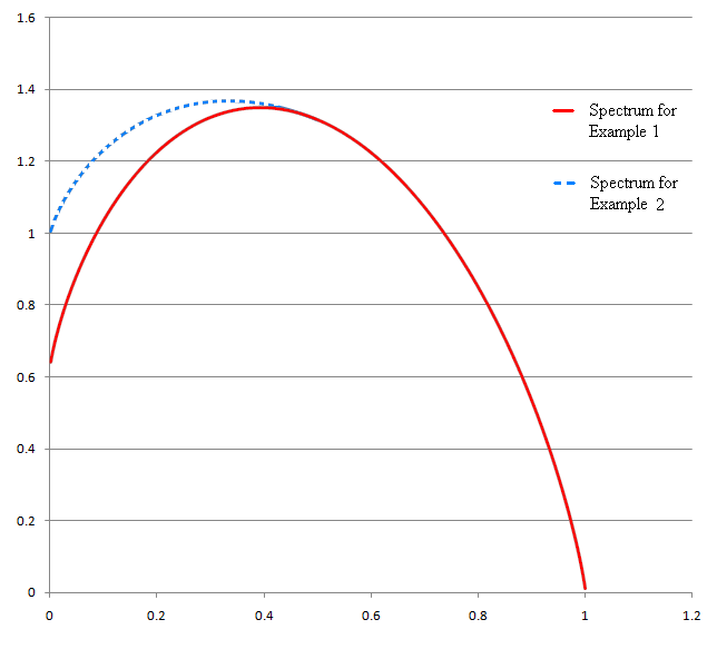
For our next example we have identical a1a_{1}, a2a_{2} and 𝒟\mathcal{D}, along with a potential φ\varphi which is prima facie very close to our previous one. Indeed for α≥12\alpha\geq\frac{1}{2} the spectra for the two examples coincide (see Figure 2). However our next example has a point of non-analyticity at α=12\alpha=\frac{1}{2} and for α<12\alpha<\frac{1}{2} the two packing spectra are very different. In particular, the packing spectrum attains the packing dimension of Λ\Lambda and so rises above the Hausdorff spectrum.

Example 2.

Take a=3a=3, b=2b=2 and 𝒟={(0,0),(1,1),(2,0)}\mathcal{D}=\left\{(0,0),(1,1),(2,0)\right\} and φ:Λ→ℝ\varphi:\Lambda\rightarrow\mathbb{R} defined by

φ⁡(ω)={1​ if ​ω1=(2,0)0​ if ​ω1≠(2,0)\varphi(\omega)=\begin{cases}1\text{ if }\omega_{1}=(2,0)\\ 0\text{ if }\omega_{1}\neq(2,0)\\ \end{cases}
dim𝒫​Eφ∘Π​(α)={−α​log⁡α−(1−α)​log⁡(1−α)−α​log⁡2log⁡3+1​ for ​α≤12−α​log⁡α−(1−α)​log⁡(1−α)log⁡2+(1−α)​log⁡2log⁡3​ for ​α>12.\displaystyle\mbox{dim}_{\mathcal{P}}E_{\varphi\circ\Pi}(\alpha)=\begin{cases}\frac{-\alpha\log\alpha-(1-\alpha)\log(1-\alpha)-\alpha\log 2}{\log 3}+1\text{ for }\alpha\leq\frac{1}{2}\\ \frac{-\alpha\log\alpha-(1-\alpha)\log(1-\alpha)}{\log 2}+(1-\alpha)\frac{\log 2}{\log 3}\text{ for }\alpha>\frac{1}{2}.\end{cases}

Moreover, α↦dim𝒫​Eφ​(α)\alpha\mapsto\mbox{dim}_{\mathcal{P}}E_{\varphi}(\alpha) is non-analytic and attains the full packing dimension dim𝒫​(Λ)\mbox{dim}_{\mathcal{P}}(\Lambda) at its maximum.

Proof.

Note that

sup{∑i=13−pilogpi:pi∈[0,1],∑i=13pi=1,p1=α}=−αlogα−(1−α)log(1−α2)\displaystyle\sup\left\{\sum_{i=1}^{3}-p_{i}\log p_{i}:p_{i}\in[0,1],\sum_{i=1}^{3}p_{i}=1,p_{1}=\alpha\right\}=-\alpha\log\alpha-(1-\alpha)\log\left(\frac{1-\alpha}{2}\right)
sup{∑i=12−pilogpi:pi∈[0,1],∑i=12pi=1,p1≥α}={log⁡2​ for ​α≤12−α​log⁡α−(1−α)​log⁡(1−α)​ for ​α>12.\displaystyle\sup\left\{\sum_{i=1}^{2}-p_{i}\log p_{i}:p_{i}\in[0,1],\sum_{i=1}^{2}p_{i}=1,p_{1}\geq\alpha\right\}=\begin{cases}\log 2\text{ for }\alpha\leq\frac{1}{2}\\ -\alpha\log\alpha-(1-\alpha)\log(1-\alpha)\text{ for }\alpha>\frac{1}{2}\end{cases}.

Moreover, since φ\varphi is locally constant the following suprema are both attained by Bernoulli measures,

sup{hμ(σ):μ∈ℬσ(Σ),∫φdμ=α}\displaystyle\sup\left\{h_{\mu}(\sigma):\mu\in\mathcal{B}_{\sigma}(\Sigma),\int\varphi d\mu=\alpha\right\}
sup{hμ∘χ2−1(σv):μ∈ℬσ(Σ),∫φdμ=α}.\displaystyle\sup\left\{h_{\mu\circ\chi_{2}^{-1}}(\sigma_{v}):\mu\in\mathcal{B}_{\sigma}(\Sigma),\int\varphi d\mu=\alpha\right\}.

Thus, applying Theorem 7 we have

dim𝒫​Eφ∘Π​(α)={−α​log⁡α−(1−α)​log⁡(1−α)−α​log⁡2log⁡3+1​ for ​α≤12−α​log⁡α−(1−α)​log⁡(1−α)log⁡2+(1−α)​log⁡2log⁡3​ for ​α>12.\displaystyle\mbox{dim}_{\mathcal{P}}E_{\varphi\circ\Pi}(\alpha)=\begin{cases}\frac{-\alpha\log\alpha-(1-\alpha)\log(1-\alpha)-\alpha\log 2}{\log 3}+1\text{ for }\alpha\leq\frac{1}{2}\\ \frac{-\alpha\log\alpha-(1-\alpha)\log(1-\alpha)}{\log 2}+(1-\alpha)\frac{\log 2}{\log 3}\text{ for }\alpha>\frac{1}{2}\end{cases}.

Consequently, α↦dim𝒫​Eφ​(α)\alpha\mapsto\mbox{dim}_{\mathcal{P}}E_{\varphi}(\alpha) is non-analytic. This follows from the fact that the functions

α↦−α​log⁡α−(1−α)​log⁡(1−α)−α​log⁡2log⁡3+1\displaystyle\alpha\mapsto\frac{-\alpha\log\alpha-(1-\alpha)\log(1-\alpha)-\alpha\log 2}{\log 3}+1
α↦−α​log⁡α−(1−α)​log⁡(1−α)log⁡2+(1−α)​log⁡2log⁡3\displaystyle\alpha\mapsto\frac{-\alpha\log\alpha-(1-\alpha)\log(1-\alpha)}{\log 2}+(1-\alpha)\frac{\log 2}{\log 3}

have distinct second derivatives at α=12\alpha=\frac{1}{2}. It also follows from our expression for dim𝒫​Eφ​(α)\mbox{dim}_{\mathcal{P}}E_{\varphi}(\alpha), together with 2, that the full packing dimension is attained at α=13\alpha=\frac{1}{3}. ∎

Refer to caption
Figure 2. The packing spectra for examples 11 and 22. The spectrum in Example 11 is given by the red line. Example 22 has a second order phase transition at α=12\alpha=\frac{1}{2}. For α≤12\alpha\leq\frac{1}{2} the spectrum in Example 2 is given by the broken blue line. For α>12\alpha>\frac{1}{2} the two spectra coincide and are both given by the red line.

7. Generalisations and open questions

In this section we note some Corollaries to Theorem 6 and 7. The first concerns sets of divergent points. Usually one considers sets of points for which the Birkhoff average converges to a given value. However, given any non-empty closed convex subset A⊆A⁡(φ)A\subseteq A(\varphi) one may consider the set Eφ​(A)E_{\varphi}(A) of points x∈Λx\in\Lambda for which the set of accumulation points for the sequence (An​(φ)​(x))n∈ℕ(A_{n}(\varphi)(x))_{n\in\mathbb{N}} is equal to AA. In the conformal setting both dimℋ​Eφ​(A)\mbox{dim}_{\mathcal{H}}E_{\varphi}(A) and dim𝒫​Eφ​(A)\mbox{dim}_{\mathcal{P}}E_{\varphi}(A) have been well studied in a series of papers due to Olsen and Winter [Ol1], [OlWi], [Ol2], [Ol3]. This follows work by Barreira and Schmeling [BSch] showing that, given finitely many continuous potentials φ1,⋯,φN\varphi_{1},\cdots,\varphi_{N} on a conformal repeller Λ\Lambda for which each A⁡(φi)A(\varphi_{i}) consists of at least two points, the Hausdorff dimension (and hence packing dimension) of the set of all points for which none of the Birkhoff averages for φ1,⋯,φN\varphi_{1},\cdots,\varphi_{N} converge is of full Hausdorff dimension. We note that [Ol3, Theorem 4.3] implies that the set of points x∈Λx\in\Lambda for which the Birkhoff average (An​(φ)​(x))n∈ℕ(A_{n}(\varphi)(x))_{n\in\mathbb{N}} does not converge for any continuous potential φ\varphi for which A⁡(φ)A(\varphi) consists of at least two points again, has full Hausdorff dimension. By a similar argument, along with some ideas from [KP], one can extend this result to self-affine Sierpiński sponges.

One application of Theorem 7 is to determine the packing dimension of the sets Eφ​(A)E_{\varphi}(A) for self-affine Sierpiński sponges. We define, for k=1,⋯,dk=1,\cdots,d,

(7.1) Hk​(f,φ,A)\displaystyle H^{k}(f,\varphi,A) :⁣=\displaystyle:= sup{hμ∘πk−1(fk):μ∈ℳ(f,Λ),∫φdμ∈A}.\displaystyle\sup\left\{h_{\mu\circ\pi_{k}^{-1}}(f_{k}):\mu\in\mathcal{M}(f,\Lambda),\int\varphi d\mu\in A\right\}.
Theorem 8.

Let Λ\Lambda be a self-affine Sierpiński sponge. Let φ:Λ→ℝN\varphi:\Lambda\rightarrow\mathbb{R}^{N} be some continuous potential. Then given any non-empty closed convex subset A⊆A⁡(φ)A\subseteq A(\varphi) we have

dim𝒫​Eφ​(A)=H1​(f,φ,A)log⁡a1+∑k=2d(1log⁡ak−1log⁡ak−1)​Hk​(f,φ,A).\mbox{dim}_{\mathcal{P}}{E_{\varphi}(A)}=\frac{H^{1}(f,\varphi,A)}{\log a_{1}}+\sum_{k=2}^{d}\left(\frac{1}{\log a_{k}}-\frac{1}{\log a_{k-1}}\right)H^{k}(f,\varphi,A).

In contrast very little is known concerning the Hausdorff dimension of Eφ​(A)E_{\varphi}(A) for self-affine Λ\Lambda, aside from the special case where AA is a singleton, and it would be very interesting to see if one could obtain a formula for dimℋ​Eφ​(A)\mbox{dim}_{\mathcal{H}}E_{\varphi}(A) for arbitrary non-empty closed convex subsets of ℳ⁡(Λ,f)\mathcal{M}(\Lambda,f).

Theorem 7 also implies the some results concerning the packing spectrum for the local dimension of a Bernoulli measure on a self-affine Sierpiński sponge. To each Bernoulli measure μ\mu on Σ\Sigma we associate the corresponding probability vector (pi1⋯id)(i1,⋯,id)∈𝒟(p_{i_{1}\cdots i_{d}})_{(i_{1},\cdots,i_{d})\in\mathcal{D}} in the usual way. Given t∈{1⋯,d}t\in\{1\,\cdots,d\} we let pi1⋯itp_{i_{1}\cdots i_{t}} denote the sum of all pj1⋯jdp_{j_{1}\cdots j_{d}} for which (j1,⋯,jt)=(i1,⋯,it)(j_{1},\cdots,j_{t})=(i_{1},\cdots,i_{t}).

For j=1,⋯,dj=1,\cdots,d we define a potential Pj:Σ→ℝP_{j}:\Sigma\rightarrow\mathbb{R} by

(7.2) Pj​(ω):={log⁡pχj​(ω1)/pχj+1​(ω1)log⁡aj​ if ​j≠dlog⁡pχd​(ω1)log⁡ad​ if ​j=d.\displaystyle P_{j}(\omega):=\begin{cases}\frac{\log p_{\chi_{j}(\omega_{1})}/p_{\chi_{j+1}(\omega_{1})}}{\log a_{j}}\text{ if }j\neq d\\ \frac{\log p_{\chi_{d}(\omega_{1})}}{\log a_{d}}\text{ if }j=d.\end{cases}

Clearly var1​(Pj)=0\text{var}_{1}(P_{j})=0 for each jj and as such PjP_{j} is continuous. Let P:Σ→ℝdP:\Sigma\rightarrow\mathbb{R}^{d} denote the potential ω↦(Pj​(ω))j=1d\omega\mapsto(P_{j}(\omega))_{j=1}^{d}. We shall assume the Very Strong Separation Condition (see [Ol4, Condition (II)]).

Lemma 7.1.

Suppose that μ\mu is a Bernoulli measure on a self-affine Sierpiński sponge which satisfies the Very Strong Separation Condition. Then for all x=Π⁡(ω)∈Λx=\Pi(\omega)\in\Lambda we have

(7.3) limr→∞log⁡μ⁡(B⁡(x,r))log⁡r=∑j=1d1⌈λj​n⌉​∑l=0⌈λj​n⌉−1Pj​(σl​ω).\lim_{r\rightarrow\infty}\frac{\log\mu(B(x,r))}{\log r}=\sum_{j=1}^{d}\frac{1}{\lceil\lambda_{j}n\rceil}\sum_{l=0}^{\lceil\lambda_{j}n\rceil-1}P_{j}(\sigma^{l}\omega).
Proof.

See [Ol4, Theorem 6.2.2]. ∎

Olsen [Ol4, Conjecture 4.1.7] conjectured that the packing spectrum of a Bernoulli measure on a self-affine Sierpiński sponge is given by the Legendre transform of an certain auxiliary function (see [Ol4, Section 3.1] for details). In particular, this conjecture would imply that the packing spectrum for local dimension always peaks at the full packing dimension of the attractor Λ\Lambda (see [Ol4, Theorem 3.3.2 (ix)] and note that γ⁡(0)=dim𝒫​Λ\gamma(0)=\mbox{dim}_{\mathcal{P}}\Lambda by Theorem 2). Theorem 7 provides us with the following counterexample.

Example 3.

Take a1=4a_{1}=4, a2=3a_{2}=3 and 𝒟={(0,0),(2,2),(3,0)}\mathcal{D}=\left\{(0,0),(2,2),(3,0)\right\} and let ν\nu be the Bernoulli measure obtained by taking p00=p30=1/4p_{00}=p_{30}=1/4 and p22=1/2p_{22}=1/2. Let αmin:=log⁡2/log⁡3\alpha_{\min}:=\log 2/\log 3 and αmax:=log⁡2/log⁡3+1/2\alpha_{\max}:=\log 2/\log 3+1/2 and for all α∈[αmin,αmax]\alpha\in[\alpha_{\min},\alpha_{\max}] we define ρ⁡(α):=2​(α−log⁡2/log⁡3).\rho(\alpha):=2\left(\alpha-\log 2/\log 3\right). Then, dimℋ​(Λ)<dim𝒫​(Λ)\mbox{dim}_{\mathcal{H}}(\Lambda)<\mbox{dim}_{\mathcal{P}}(\Lambda). However, for all α∈[αmin,αmax]\alpha\in[\alpha_{\min},\alpha_{\max}],

dim𝒫​Dν​(α)=dimℋ​Dν​(α)=−ρ⁡(α)​log⁡ρ⁡(α)−(1−ρ⁡(α))​log⁡(1−ρ⁡(α))log⁡4+12​(1−ρ⁡(α)).\displaystyle\mbox{dim}_{\mathcal{P}}D_{\nu}(\alpha)=\mbox{dim}_{\mathcal{H}}D_{\nu}(\alpha)=\frac{-\rho(\alpha)\log\rho(\alpha)-(1-\rho(\alpha))\log(1-\rho(\alpha))}{\log 4}+\frac{1}{2}(1-\rho(\alpha)).
Proof.

Theorem 2 implies dimℋ​(Λ)<dim𝒫​(Λ)\mbox{dim}_{\mathcal{H}}(\Lambda)<\mbox{dim}_{\mathcal{P}}(\Lambda). Applying Lemma 7.1 we see that for all α∈[αmin,αmax]\alpha\in[\alpha_{\min},\alpha_{\max}] we see that Π​(ω)∈Dν​(α)\Pi(\omega)\in D_{\nu}(\alpha) if and only if

(7.4) 𝒱⁡(ω)⊆{μ∈ℳσ​(Σ):μ⁡([(0,0)])+μ⁡([3,0])=ρ⁡(α)}.\mathcal{V}(\omega)\subseteq\left\{\mu\in\mathcal{M}_{\sigma}(\Sigma):\mu([(0,0)])+\mu([3,0])=\rho(\alpha)\right\}.

Now proceed as in Example 1. ∎

Theorem 7 also implies the following lower bound for the packing spectrum for local dimension.

Proposition 7.1.

Suppose that μ\mu is a Bernoulli measure on a self-affine Sierpiński sponge which satisfies the Very Strong Separation Condition. Then,

dim𝒫​Dμ​(α)≥sup{H1​(σ,P¯,α¯)log⁡a1+∑k=2d(1log⁡ak−1log⁡ak−1)​Hk​(f,P¯,α¯)},\mbox{dim}_{\mathcal{P}}D_{\mu}(\alpha)\geq\sup\left\{\frac{H^{1}(\sigma,\underline{P},\underline{\alpha})}{\log a_{1}}+\sum_{k=2}^{d}\left(\frac{1}{\log a_{k}}-\frac{1}{\log a_{k-1}}\right)H^{k}(f,\underline{P},\underline{\alpha})\right\},

where the supremum is taken over all α¯=(αj)j=1d∈ℝd\underline{\alpha}=(\alpha_{j})_{j=1}^{d}\in\mathbb{R}^{d} for which ∑j=1dαj=α\sum_{j=1}^{d}\alpha_{j}=\alpha.

Proof.

It follows from Lemma 7.1 that EP¯​(α¯)⊆Dμ​(α)E_{\underline{P}}(\underline{\alpha})\subseteq D_{\mu}(\alpha) for each α¯=(αj)j=1d∈ℝd\underline{\alpha}=(\alpha_{j})_{j=1}^{d}\in\mathbb{R}^{d} with ∑j=1dαj=α\sum_{j=1}^{d}\alpha_{j}=\alpha. Consequently, the result follows from Theorem 7. ∎

For a rather limited class of Bernoulli measures we obtain an equality.

Definition 7.1.

We say that a Bernoulli measure μ\mu on a self-affine Sierpiński sponge is one dimensional if there exists some k∈{1,⋯,d}k\in\{1,\cdots,d\} for which the probability vector (pi1⋯id)(i1,⋯,id)∈𝒟(p_{i_{1}\cdots i_{d}})_{(i_{1},\cdots,i_{d})\in\mathcal{D}} associated to μ\mu satisfies pi1⋯id+1−q/pi1⋯id−q=#ηq+1(𝒟)/#ηq(𝒟)p_{i_{1}\cdots i_{d+1-q}}/p_{i_{1}\cdots i_{d-q}}=\#\eta_{q+1}(\mathcal{D})/\#\eta_{q}(\mathcal{D}) for all (i1,⋯,id+1−q)∈ηq+1​(𝒟)(i_{1},\cdots,i_{d+1-q})\in\eta_{q+1}(\mathcal{D}) and all q∈{1,⋯,d−1}\{k}q\in\{1,\cdots,d-1\}\backslash\{k\} and each pi=1/#​ηd​(𝒟)p_{i}=1/\#\eta_{d}(\mathcal{D}) for i∈ηd​(𝒟)i\in\eta_{d}(\mathcal{D}), provided k≠dk\neq d.

Now if μ\mu is a one dimensional Bernoulli measure on a self-affine Sierpiński sponge then for each j≠kj\neq k PjP_{j} will be equal to an explicit constant cjc_{j}. Let P~\tilde{P} denote the potential Pk+∑j≠kcjP_{k}+\sum_{j\neq k}c_{j}.

Theorem 9.

Suppose that μ\mu is a one dimensional Bernoulli measure on a self-affine Sierpiński sponge which satisfies the Very Strong Separation Condition. Then

dim𝒫​Dμ​(α)=H1​(σ,P~,α)log⁡a1+∑k=2d(1log⁡ak−1log⁡ak−1)​Hk​(f,P~,α).\mbox{dim}_{\mathcal{P}}D_{\mu}(\alpha)=\frac{H^{1}(\sigma,\tilde{P},\alpha)}{\log a_{1}}+\sum_{k=2}^{d}\left(\frac{1}{\log a_{k}}-\frac{1}{\log a_{k-1}}\right)H^{k}(f,\tilde{P},\alpha).
Proof.

It follows from Lemma 7.1 that Dμ​(α)=EP~​(α)D_{\mu}(\alpha)=E_{\tilde{P}}(\alpha). Hence, the result follows from Theorem 7. ∎

We emphasise that the class of one dimensional Bernoulli measures is really very limited and the techniques of this paper are insufficient for determining dim𝒫​Dμ​(α)\mbox{dim}_{\mathcal{P}}D_{\mu}(\alpha) for more general classes of Bernoulli measures. The reason for this extra level of difficulty is that one is essentially dealing with a sum of Birkhoff averages taken at multiple time scales (see Lemma 7.1). It seems unlikely that the lower bound given in Proposition 7.1 is optimal. As such it remains an open question to determine the packing spectrum for local dimension on a self-affine Sierpiński sponge.

References

  • [BOS] I. Baek, L. Olsen, N. Snigireva, Divergence points of self-similar measures and packing dimension. Adv. Math. 214 (2007), no. 1, 267-287.
  • [BF] J. Barral and D. Feng, Weighted thermodynamic formalism and applications, (2009). arXiv:0909.4247v1.
  • [BM1] J. Barral and M. Mensi, Multifractal analysis of Birkhoff averages on ‘self-affine’ symbolic spaces. Nonlinearity 21 (2008), no. 10, 2409-2425.
  • [BM2] J. Barral and M. Mensi, Gibbs measures on self-affine Sierpinski carpets and their singularity spectrum. Ergodic Theory Dynam. Systems 27 (2007), no. 5, 1419–1443.
  • [BSa] L. Barreira and B. Saussol, Variational principles and mixed multifractal spectra. Trans. Amer. Math. Soc. 353 (2001), no. 10, 3919-3944.
  • [BSch] L. Barreira and J. Schmeling, Sets of non-typical points have full topological entropy and full Hausdorff dimension. Israel J. Math. 116 (2000), 29-70.
  • [Be] T. Bedford, PhD Thesis: Crinkly curves, Markov partitions and box dimension of self-similar sets. Ph.D. thesis, University of Warwick (1984).
  • [Bo] R. Bowen, Equilibrium states and the ergodic theory of Anosov diffeomorphisms. Second revised edition. Lecture Notes in Mathematics, 470. Springer-Verlag, Berlin, (2008). viii+75 pp. ISBN: 978-3-540-77605-5.
  • [Ed1] G. A. Edgar,Measure, topology, and fractal geometry. Second edition. Undergraduate Texts in Mathematics. Springer, New York, (2008). xvi+268 pp. ISBN: 978-0-387-74748-4.
  • [Ed2] G. A. Edgar, Integral, probability, and fractal measures. Springer-Verlag, New York, (1998). x+286 pp. ISBN: 0-387-98205-1
  • [Fa1] K. Falconer, The Hausdorff dimension of self-affine fractals. Math. Proc. Cambridge Philos. Soc. 103 (1988), no. 2, 339–350.
  • [Fa2] K. Falconer, Fractal geometry. Mathematical foundations and applications. Second edition. John Wiley &\& Sons, Inc., Hoboken, NJ, (2003). xxviii+337 pp. ISBN: 0-470-84861-8.
  • [Fa3] K. Falconer, Techniques in fractal geometry. John Wiley &\& Sons, Ltd., Chichester, 1997. xviii+256 pp. ISBN: 0-471-95724-0.
  • [FFW] A. Fan, D. Feng and J. Wu, Recurrence, dimension and entropy. J. London Math. Soc. (2) 64 (2001), no. 1, 229–244.
  • [FLW] D. Feng K. Lau and J. Wu, Ergodic Limits on the Conformal Repellers. Adv. Math. 169 (2002), no. 1, 58–91.
  • [GR] K. Gelfert and M. Rams, The Lyapunov spectrum of some parabolic systems. Ergodic Theory Dynam. Systems 29 (2009), no. 3, 919–940.
  • [JJOP] A. Johansson, T. Jordan, A. Oberg, and M. Pollicott, Multifractal analysis of non-uniformly hyperbolic systems. Israel J. Math. 177 (2010), 125–144.
  • [JR] T. Jordan, M. Rams, Multifractal analysis for Bedford-McMullen carpets. Math. Proc. Camb. Phil. Soc. (2011), 147-156.
  • [JS] T. Jordan, K. Simon, Multifractal Analysis of Birkhoff Averages for some Self-Affine IFS. Dyn. Syst. 22 (2007), no. 4, 469–483.
  • [Ki] J. King, The Singularity Spectrum for General Sierpinski Carpets. Adv. Math. 116 (1995), no. 1, 1-11.
  • [KP] R. Kenyon and Y. Peres, Measures of full dimension on affine-invariant sets, Ergodic Theory Dynam. Systems 16 (1996), no. 2, 307–323.
  • [Mat] P. Mattila, Geometry of Sets and Measures in Euclidean Spaces: Fractals and rectifiability. Cambridge Studies in Advanced Mathematics, 44. Cambridge University Press, Cambridge, (1995). xii+343 pp. ISBN: 0-521-46576-1; 0-521-65595-1.
  • [McM] C. McMullen, The Hausdorff Dimension of General Sierpinski Carpets. Nagoya Math. J. 96 (1984), 1–9.
  • [Ni] O. Nielsen, The Hausdorff and packing dimensions of some sets related to Sierpiński carpets. Canad. J. Math. 51 (1999), no. 5, 1073–1088.
  • [Ol1] L. Olsen, Multifractal analysis of divergence points of deformed measure theoretical Birkhoff averages. J. Math. Pures Appl. (9) 82 (2003), no. 12, 1591–1649.
  • [Ol2] L. Olsen, Multifractal analysis of divergence points of deformed measure theoretical Birkhoff averages III. Aequationes Math. 71 (2006), no. 1-2, 29–53.
  • [Ol3] L. Olsen, Multifractal analysis of divergence points of deformed measure theoretical Birkhoff averages. IV: Divergence points and packing dimension. Bull. Sci. Math. 132 (2008), no. 8, 650–678.
  • [Ol4] L. Olsen, Self-affine multifractal Sierpiński sponges in ℝd\mathbb{R}^{d}. Pacific J. Math. 183 (1998), no. 1, 143–199.
  • [OlWi] L. Olsen, S. Winter, Multifractal analysis of divergence points of deformed measure theoretical Birkhoff averages II: Non-linearity, divergence points and Banach space valued spectra. Bull. Sci. Math. 131 (2007), no. 6, 518–558.
  • [Per] Y. Peres, The packing measure of self-affine carpets. Math. Proc. Camb. Phil. Soc. 115 (1994), no. 3, 437–450.
  • [Pes] Y. Pesin, Dimension Theory in Dynamical Systems. Contemporary views and applications. Contemporary views and applications. Chicago Lectures in Mathematics. University of Chicago Press, Chicago, IL, 1997. xii+304 pp. ISBN: 0-226-66221-7; 0-226-66222-5.
  • [PW1] Y. Pesin, H. Weiss, The Multifractal Analysis of Birkhoff Averages and Large Deviations. Global analysis of dynamical systems, 419–431, Inst. Phys., Bristol, 2001.
  • [PW2] Y. Pesin, H. Weiss, The Multifractal Analysis of Gibbs Measures: Motivation, mathematical foundation and examples. Chaos 7 (1997), no. 1, 89–106.
  • [Wa] P. Walters, An Introduction to Ergodic Theory. Graduate Texts in Mathematics, 79. Springer-Verlag, New York-Berlin, (1982). ix+250 pp. ISBN: 0-387-90599-5.