Molecular Communication Using Brownian Motion with Drift
Abstract
Inspired by biological communication systems, molecular communication has been proposed as a viable scheme to communicate between nano-sized devices separated by a very short distance. Here, molecules are released by the transmitter into the medium, which are then sensed by the receiver. This paper develops a preliminary version of such a communication system focusing on the release of either one or two molecules into a fluid medium with drift. We analyze the mutual information between transmitter and the receiver when information is encoded in the time of release of the molecule. Simplifying assumptions are required in order to calculate the mutual information, and theoretical results are provided to show that these calculations are upper bounds on the true mutual information. Furthermore, optimized degree distributions are provided, which suggest transmission strategies for a variety of drift velocities.
I Introduction
Communications research has almost exclusively focused on systems based on electromagnetic propagation. However, at scales considered in nano-technology, it is not clear that these methods are viable. Inspired by the chemical-exchange communication performed by biological cells, this paper considers molecular communication [1], in which information is transmitted by an exchange of molecules. Specifically we consider the propagation of individual molecules between closely spaced transmitters and receivers, both immersed in a fluid medium. The transmitter encodes a message in the pattern of release of the molecules into the medium; these molecules then propagate to the receiver where they are sensed. The receiver then attempts to recover the message by observing the pattern of the received molecules.
It is well known that microorganisms exchange information by molecular communication, with quorum sensing [2] as but one example, where bacteria exchange chemical messages to estimate the local population of their species. The biological literature on molecular communication is vast, but there has been much recent work concerning these systems as engineered forms of communication. Several recent papers have described the design and implementation of engineered molecular communication systems, using methods such as: exchanging arbitrary molecules using Brownian motion in free space [3]; exploiting gap junctions between cells to exchange calcium ions [4, 5]; and using microtubules and molecular motors to actively drive molecules to their destination [6, 7]. A comprehensive overview of the molecular communication system is also given by [8, 9] and the references therein.
Given this engineering interest, it is useful to explore the theoretical capabilities of molecular communication systems. To the authors’ knowledge, the earliest effort towards information-theoretic analysis of these channels was given in [10], which examined information flow in continuous diffusion. In [11, 12], physical models and achievable bounds on information rate were provided for diffusion-based systems. Information rates were provided in [13, 14] for the case where the receiver chemically “reacts” with the molecules and form “complexes”. In [15], it was shown that the additive white Gaussian noise (AWGN) is appropriate for diffusion-based counting channels. Information-theoretic results have also been obtained for specific systems, such as propagation along microtubules [16, 17] and continuous diffusion [18]. All these studies indicate that useful information rates can be obtained, although much lower per unit time than in electrical communication; this is not surprising, since chemical processes are far slower than electrical processes. It is worth pointing out that these results build on theoretical work in Poisson and queue-timing channels [19, 20], which is an active area of research in information theory.
In any communication system, the potential rate of communication is determined by the characteristics of the channel. We consider molecular propagation in a fluid medium, governed by Brownian motion and, potentially, a mean drift velocity. Our model is therefore applicable to communications in, e.g., a blood vessel. This drift velocity is a key difference between our work and [11, 12], which considered a purely diffusion channel. Furthermore, we consider two cases - a single and two molecules being released. In this regard, it is worth emphasizing the preliminary and conceptual nature of this work. The long-term goal of this work is to understand the role of both timing and the number of molecules (‘amplitude’). Thus, the contributions of this paper include:
- •
Calculation and optimization, under some simplifying assumptions, of mutual information in Brownian motion with drift, where the transmitter uses pulse-position modulation;
- •
Optimization of the degree distributions related to two transmit molecules; and
- •
Demonstration (via theoretical results) that our simplified mutual information calculation is an upper bound on the true mutual information of any practical implementation of this system.
Our optimized degree distributions reveal interesting features of these channels, suggesting transmission strategies for system designers.
The paper is organized as follows. In Section II we describe the system under consideration, in which the propagation of the molecule is analyzed and the probability distribution function of the absorption time is derived. In Section III, we characterize the maximum information transfer per molecule, for the case where information is encoded in the time of release of the molecule, and the case of two molecules. In Section IV, numerical and theoretical results arising from these models (including optimized degree distributions) are presented. The paper wraps up with some conclusions and suggestions for future work.
II System Model
II-A Communication model
The communication model we consider is shown in Figure 1. The subsystems which make up the molecular communication system are:
- 1.
Transmitter. The transmitter is a source of identical molecules. It encodes a message in the time of dispersal of these molecules. We will assume that the transmitter can control precisely the time of dispersal of these molecules but does not influence the propagation of these molecules once dispersed.
- 2.
Propagation medium. The molecules propagate between transmitter and receiver in a fluid medium. The propagation is modeled as Brownian motion, and is characterized by two parameters: the drift velocity and the diffusion constant. These in turn depend on the physical properties of the fluid medium. The trajectories of different molecules are assumed to be independent of one another.
- 3.
Receiver. In this paper, the propagation of the molecule is assumed to be one dimensional. When it arrives at the receiver, the dispersed molecule is absorbed by the receiver and is removed from the medium. The receiver makes an accurate measurement of the time when it absorbs the molecule. It uses this information to determine the message sent by the transmitter.
- 4.
Transmission of information. The transmitter can encode information in either the time of dispersal of the molecules, or the number of molecules it disperses, or both.


The motion of the dispersed molecule is affected by Brownian motion; the diffusion process is therefore probabilistic and, in turn, the propagation time to the receiver is random. Even in the absence of any imperfection in the implementation of a molecular communication system, this uncertainty in the propagation time limits the maximum information rate per molecule. In this paper, we study the maximum information per molecule that the transmitter can convey to the receiver, for a certain velocity and diffusion in the fluid medium. Before proceeding to do so, we need to characterize the propagation of the molecule in the medium.
II-B Diffusion via Brownian motion
Consider the discrete-time, discrete-space propagation model in Figure 2(a). Let denote the position of the particle at time . Let denote the probability mass function (pmf) of the position of the particle at time , given that it was dispersed in the fluid medium at position at time . Assume that the fluid medium is static, and so the particle disperses in either of the directions with equal probability. If is the probability that the particle moves from position to position in one time unit, and is the probability that it moves from position to , then this situation is the case when . It is easy to see that obeys the equation
| (1) |
which states that if a particle at time is at position , then at time , it should have been at position or , where is the distance between two slices of space. This formulation of Brownian motion is analogous to a Wiener process, where distinct increments of the motion are independent from each other.
Equation (1) can be re-written as
| (2) | |||||
When and , the difference equation becomes a continuous time differential equation, yielding a probability distribution function (pdf) for the position of the particle, given by,
| (3) |
Now, considering a continuous time Brownian motion , the probability density function of the position of the particle can be modeled by the diffusion equation
| (4) |
where is the diffusion constant, whose value is dependent on the viscosity of the fluid medium. Note that the above equation characterizes only the ‘-coordinate’ of the position of the molecule. Solutions to this equation are well known.
Equation (4) characterizes the motion of the particle in a macroscopically static medium. The more general and useful case is that of a fluid medium is in motion with a mean drift velocity . Consider a frame of reference which is moving with the same velocity. In this frame, the fluid medium is static and hence the diffusion of the particle should obey Equation (4). Let
be the new coordinate system, and without loss of generality, assume . Let
then
In the static frame of reference, the differential equation can be written as
| (5) | |||||
which simplifies to
| (6) |
Assume that there is no absorbing boundary (receiver) and that the fluid medium extends from to . The probability density function of the location of the particle can be obtained by solving the differential Equation (6) with boundary conditions and The solution to (6) is given by [21]
| (7) |
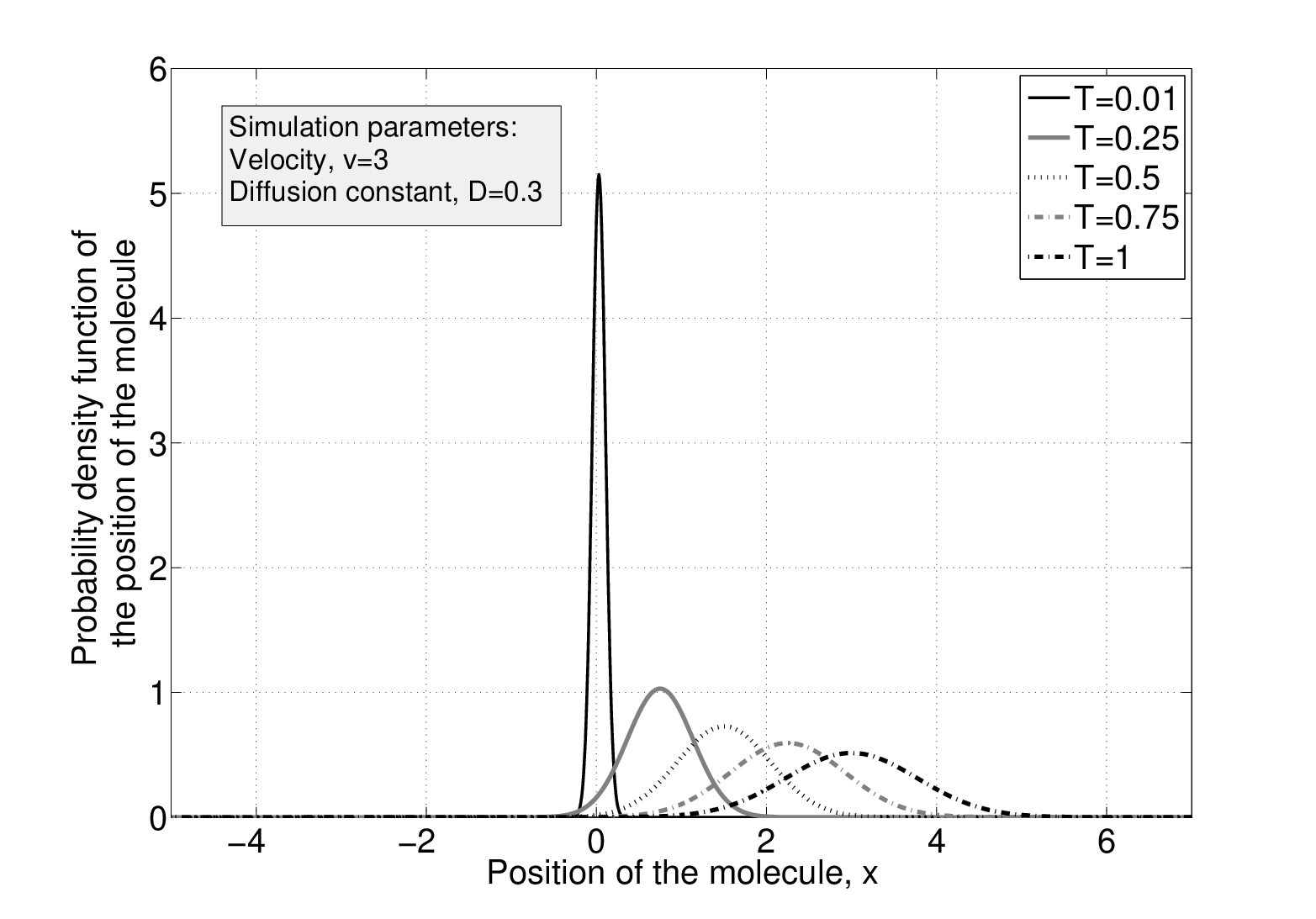
Equation (7) states that, for every , the probability density function (pdf) is a Gaussian centered at with variance . As expected, the expected location of the particle drifts along the direction of flow of the fluid medium with velocity . Figure 3 plots for the case when and . Furthermore, for any transmitter point and transmit time , we have that
| (8) |
As expected, Brownian motion satisfying (7)-(8) is a Wiener process with drift.
Now, consider the case when there is an absorbing surface (receiver) at . The particle is absorbed and is removed from the system when it hits the absorbing surface. For such a system, to solve for , we need to solve the differential equation in (6) with the following boundary conditions.
- •
For . The probability density function has a physical interpretation only for . In this region, we require it to be a delta function at centered at .
- •
.
- •
. Condition imposed by the absorbing surface.
The solution to the differential equation can be computed using the method of images, it is given by:
| (9) |
II-C Distribution of Absorption Time
Recall from Section II that the receiver senses the particles only when they arrive, at which time they are absorbed and removed from the system. Thus, for the purposes of this paper, the most important feature of the Brownian motion expressed in (6)-(8) is the first passage time at the destination. For a Brownian motion , and an absorbing boundary located at position , the first passage time at the barrier is defined as
| (10) |
In Figure 2(b), the simulated trajectories of six particles, modeled as a random walk, through a medium are plotted. The particles were all released at , three at time and three at time 400, into a fluid medium that had a positive drift velocity. The receiver is located at . Notice the large variation in the absorption times. Among the particles released at , one gets absorbed at , other at , and another does not get absorbed even by . Furthermore, this plot shows how particles can get absorbed in an order different from the order in which they were released. It is therefore important to understand the variation in the propagation times of the particle.
The derivation of the first passage time for our case is given in [22]. Here, we repeat briefly the steps involved. At a given time , the probability that the particle has not yet been absorbed is given by
(t) is the probability that the particle has not been absorbed until time . The probability that the particle has been absorbed before is given by . Hence, the probability density function of the absorption time is .
| (11) | |||||
To summarize, (11) gives the probability density function of the absorption time of a particle released in a fluid medium with diffusion constant , at a distance from the receiver, when the fluid has a constant velocity . Note that this equation is valid only for positive drift velocities, i.e., when the receiver is downstream from the transmitter. Since our communication is based largely on the time of transmission (and reception), this pdf characterizes the uncertainty in the channel, and plays a role similar to that of the noise distribution in an additive noise channel. Some example plots of this function are given in Figure 4.

III Mutual Information
The transmitter encodes the message in the time of release of molecules and possibly the number of molecules. Based on the number and the time of absorption of the molecules, the receiver decodes the transmitted information. This section develops the mutual information between the transmitter and receiver for two cases: with a single transmitted molecule and two molecules whose release times can be chosen independently. For a given information transmission strategy at the transmitter (called the input distribution in the information theoretic literature), the mutual information is also the maximum rate at which information may be conveyed using that strategy. (Mutual information is related to but distinct from the capacity, which is the maximum mutual information over all possible input distributions.)
III-A Overview
In a traditional wireline communication system, receiver noise causes uncertainty in the reception, limiting the rate at which information can be conveyed. However, as discussed before, the uncertainty in the propagation time is a major bottleneck to the information transfer in molecular communication. This uncertainty in the propagation time also means that the order in which molecules are received at the receiver need not be the order in which they were transmitted. This will result in “inter-block interference”. This is a serious impairment in the low velocity regime, where the pdf of the absorption time decays very slowly, making inter-block interference more likely.
In this paper, we ignore inter-block interference and assume that the clocks are synchronized. Developing techniques for both issues are significant works in themselves and outside the scope of this paper. So our results are most relevant to system in a fluid with some significant drift; further, as we show in Section V, our results can be used to obtain upper bounds on both mutual information and capacity for any drift velocity.
The channel here falls under a class of timing channels, channels where the mode of communication is through the timings of various events. The capacity of such channels are usually more difficult to characterize. A celebrated result in this field is the computation of the capacity of a single server queuing system [20]. The molecular communication channel can be modeled as a queuing system, i.e., an infinite server queuing system where the service time of a server is a random variable with distribution same as the pdf of the absorption time. To our knowledge, the exact capacity of such a channel has not been computed to date.
III-B Single molecule: Pulse position modulation
We first analyze the case of the transmitter releasing just a single molecule. In such a scenario, it can encode information only in the time of release of the molecule. The transmitter releases the molecule (or not at all) in the beginning of one of time slots, each of unit duration (i.e., in arbitrary units); this action on the part of the transmitter is called a channel use. This molecule then propagates through the medium and is absorbed by the receiver in a later time slot. The receiver then guesses the time slot in which the molecule was released. This is a form of pulse-position modulation (PPM).
Given that it has choices, the transmitter can encode a maximum of bits of information per channel use, though in practice much less due to the uncertain arrival times of the molecules. For instance, suppose the velocity of the fluid medium is high enough so that the particle gets absorbed by the receiver in time slots with very high probability. In this case, one transmission strategy would be to emit a molecule in one of time slots (each separated by slots), since inter-block interference would thus occur with very low probability, and the transmitted information would arrive without distortion. For such an ideal system, we can transmit information at a rate of bits per channel use. However, more practical and interesting is the less than ideal case with lower velocities.
In this paper we neglect inter-block interference, i.e., we assume that the receiver waits for enough time slots , to ensure that the molecule propagates to the receiver with high probability. Here is chosen such that this probability is 0.999. Further, we assume that the receiver sampling rate is . This provides both a digital input/output system while maintaining fairly high accuracy of the received time. Both these parameters could be changed as required.
III-C Mutual information as an optimization problem
Having dealt with preliminaries, we now derive the maximum possible mutual information, here as an optimization problem. Define a random variable to denote the time slot in which the transmitter releases the molecule. Assume that the transmitter releases the particle at the beginning of the slot () with probability . With probability , the transmitter does not release the particle. Let denote the time slot in which the receiver absorbs the molecule. For the time being, we allow to range between and , we will see shortly that this is not required. Also, let denote the event that the molecule is never received. Since in our idealized case, the receiver waits for a sufficiently long time, the event of is the same event that the molecule is not transmitted. Assume that the duration of the time slot is .
Let denote the probability that the particle gets absorbed before time given that it was released at time 0, i.e., is the integral of the pdf in (11). Denote by the probability that the particle arrives in the time slot, given that it was released at time 0, which is equal to ; . Let denote the entropy of random variable and let represent the binary entropy function, where
| (12) |
We now proceed to calculate the mutual information between the random variables and .
| (13) | |||||
| (14) | |||||
| (15) | |||||
As seen in Figure 4, the sequence is a an eventually decreasing sequence. The rate of decay depends on the values of the drift velocity and the diffusion coefficient . The summations in (15) can, therefore, be terminated for some large enough .
The expression for mutual information is a non-negative weighted sum of concave functions plus a constant. Hence, the mutual information is a concave function of the input distribution . Finding the degree distributions, the values for s which maximize the entropy, is therefore a concave optimization problem. Standard convex optimization techniques can therefore be used to solve for the input probability distribution which maximizes the mutual information efficiently, in particular, the Blahut-Arimoto algorithm [23, 24].
As a special case, suppose that we were to convey information only in the time of release of the molecule, i.e., we require the molecule to be transmitted. The derivation of mutual information is very similar to the derivation above. Mutual information can then be expressed as
| (16) |
and, again, the optimal degree distribution can be obtained through concave optimization.
III-D Two molecules
In the work so far we have considered only the propagation of a single molecule and the focus was on PPM-based communication. We now take a step toward involving amplitude wherein the transmitter can release two identical molecules. The analysis is simplified by assuming that the propagation paths of these two molecules are independent. The transmitter releases each of these molecules in one of the time slots or chooses not to release it. Based on the arrival times of these molecules at the receiver, the receiver estimates their release times. However, because of the nature of the diffusion medium, different molecules can take different times to propagate to the receiver. Hence, the molecules can be absorbed in a different order than in which they were released: a key difference between this channel and traditional additive noise channels. As a result, the amount of information that can be conveyed through the medium with two indistinguishable molecules, as we will shortly see, is less than twice the amount of the information that can be conveyed using a single molecule.
To obtain the maximum mutual information, let be the time slot in which the first particle is released, be the time slot in which the second particle is released. Let , and be the time slots in which the first and second particles are received. For notational convenience, if a particle is not released, we denote it by a release in slot 0. Likewise, if a particle is not received at the receiver, we denote it by a reception in time slot 0.
The probability mass function of the reception times , and the conditional probability mass function of the reception times given the transmission times can be expressed in terms of the conditional probability mass function of the reception time of one molecule, given its transmission time . Let represent .
The term in the above equations accounts for the event that the molecule released later gets absorbed before the molecule which is released earlier. The mutual information between the variables and can now be written in terms of these probability mass functions. Note that in the above derivation, we have assumed that for is defined as zero.
Using these equations, we can frame the mutual information maximization as another optimization problem. The optimization is to be done over the upper triangular matrix , where each entry in the matrix is a positive number and all the entries sum to one. The mutual information is a concave function of the optimization variables . The exact expression is tedious to write, and is omitted here.
IV Results
The well known Blahut-Arimoto algorithm [23, 24] is used to compute, numerically, the input distribution that maximizes the mutual information in each of the different scenarios. The distance from the sender to the receiver, is set to one unit in all the results presented here.
IV-A Release of a single molecule
When one molecule is to be released, information can be conveyed in whether it is released or not, and if released, the slot number in which it is released.
Case when the molecule can be released in one of the slots, or not at all
In Figure 5, we plot the mutual information as a function of velocity, for two different sets of diffusion coefficients, 0.05, representing the low diffusion scenario, and a high diffusion constant 0.2. We have two sets of plots in the figure, one for the case where we have two slots in which we can release the molecule, or choose not to release it, and another, where we have four time slots. Also, we give the input distribution at which the mutual information is maximized at the two extreme values of velocity.
From the figure, it is evident that the mutual information increases with an increase in velocity and saturates to a maximum of bits. This trend is as expected. At high velocities, the optimal, information maximizing, distribution is uniform. This is because the receiver can detect, without error, the slot in which the transmitter disperses the molecule. Also, because the receiver waits for a sufficiently long time, we can detect, without error, if a molecule was transmitted or not. Therefore, a lower limit on the mutual information is one bit. At lower velocities, timing information is completely lost and the mutual information is marginally greater than one bit.
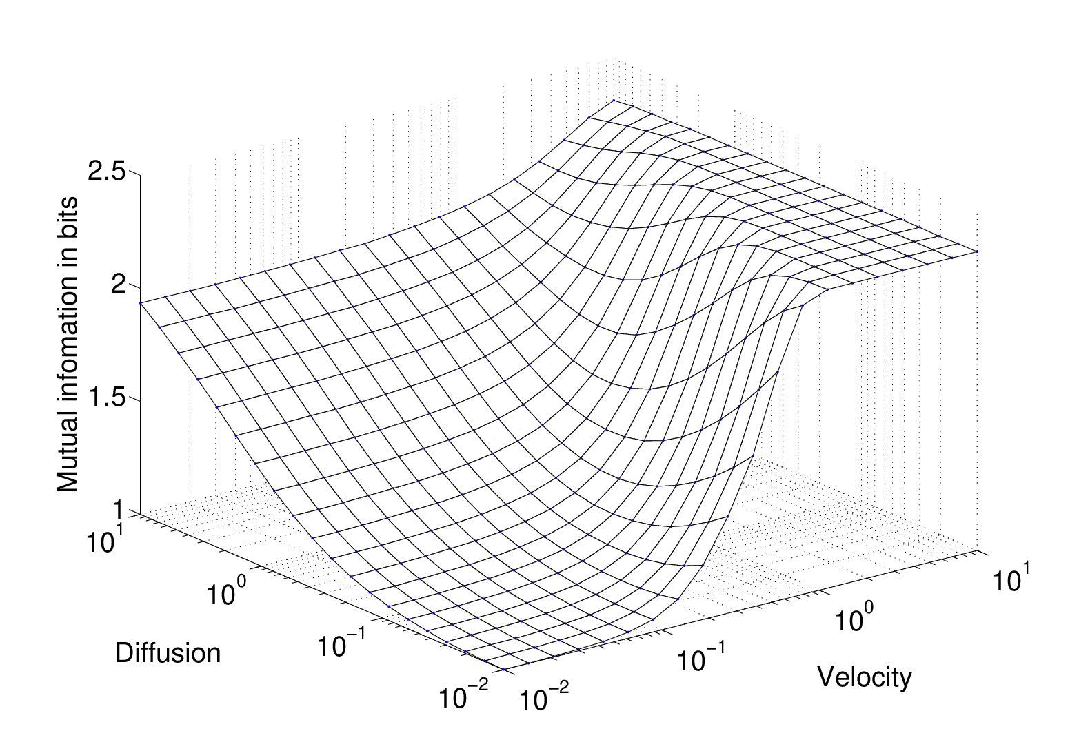
The diffusion constant is a measure of the uncertainty in the propagation time. Hence, we would expect the mutual information to be lower when the diffusion constant is high. This is indeed the case at high velocities. However, it is surprising that a higher diffusion constant results in higher mutual information at low velocities (Also refer Figure 6). This is because, at low velocities, it is the diffusion in the medium which aids the propagation of the molecule from the transmitter towards the receiver. This is illustrated in the pdf of the absorption time, shown in Figure 4. Compared to the case when the diffusion in the medium is low, the probability distribution function is more “concentrated” (lower uncertainty) when the diffusion in the medium is higher. Unfortunately, there does not seem to be a single parameter that characterizes the resulting interplay between velocity and diffusion.

Case when we do not permit the transmitter to not transmit the molecule
The information, in this scenario, is conveyed only in the time of release of the molecule. We find the input distribution which maximizes (16). The mutual information in this case is plotted in Figure 7. The maximum mutual information is now bits, which is achieved at high velocities. However, it is in the low velocity regime where the mutual information is significantly lower than the case where the transmitter is allowed to not transmit the molecule. Figure 8 compares the two scenarios.
From the results, we see that the velocity-diffusion region can be roughly classified into three regimes:
- •
A diffusion dominated region, where mutual information is relatively insensitive to the velocity; this corresponds to in Figure 5.
- •
A high-velocity region where the mutual information is insensitive to the diffusion constant; this corresponds to in Figure 5.
- •
An intermediate regime, where the mutual information is highly sensitive to the velocity and diffusion constant of the medium, in Figure 5.
In the low velocity regime, we see no significant improvement in the mutual information when we increase the number of time slots in which we can release the molecules. As expected, very little information can be conveyed in the time of release of the molecule when there is high uncertainty in the propagation time. Hence, we need to explore alternative ways of encoding message in this regime.


IV-B Release of multiple molecules
Here, we present the results of the scenario in which the transmitter is allowed to transmit at most 2 molecules. The results are presented in Figure 9. We have two sets of plots, one where the transmitter can release the molecule in one of two time slots, other, where the transmitter can release the molecule in one of four time slots. At low velocities, the mutual information is close to bits. This is because, at low velocities, any information encoded in the time of release of the molecule is lost. The receiver can however accurately estimate the number of molecules transmitted. With two molecules, the receiver can decode if the number of molecules transmitted was one or two or zero. However, this is because, we wait for infinite time at the receiver. The probability distribution function which attains the maximum mutual information at low velocities assigns, roughly, a probability of to the events of releasing one or two or no molecules.
At very high velocities, information encoded in both the time and number of molecules released is retained through the propagation. Hence, a maximum of bits can be conveyed at high velocities.
In Tables III, III and III we list the mutual information maximizing input distributions for the case of release of two molecules in two time slots. Tables VI, VI and VI list the input distributions for the case of release of two molecules in four time slots. As expected, at low velocities, the total probability of releasing one, two or zero molecules is roughly one third each. The molecules, to minimize uncertainty, are transmitted ‘far apart’.
It is however surprising to note that for reasonable velocities when two molecules are released, they are both to be released in the same time slot. This may be explained by the fact that, due to diffusion, molecules can arrive out of order and the timing information is lost. Transmitting both molecules at once avoids this confusion. This is also an important result; if this trend is to hold true for the release of multiple molecules, then we could consider only those schemes wherein all the molecules are released in one of the time slots, and where information is encoded only in the time slot in which all the molecules are released.
| 0.1424 | 0 | 0.1412 | |
| 0 | 0.1939 | 0.1921 | |
| 0 | 0 | 0.3303 |
| 0.1382 | 0 | 0.1299 | |
| 0 | 0.2113 | 0.2035 | |
| 0 | 0 | 0.3171 |
| 0.1667 | 0.1667 | 0.1667 | |
| 0 | 0.1667 | 0.1667 | |
| 0 | 0 | 0.1667 |
| 0.1395 | 0 | 0 | 0 | 0.1313 | |
| 0 | 0 | 0 | 0 | 0 | |
| 0 | 0 | 0 | 0 | 0 | |
| 0 | 0 | 0 | 0.2094 | 0.2022 | |
| 0 | 0 | 0 | 0 | 0.3176 |
| 0.1345 | 0 | 0 | 0 | 0.1256 | |
| 0 | 0.0305 | 0 | 0 | 0.0122 | |
| 0 | 0 | 0.0129 | 0 | 0 | |
| 0 | 0 | 0 | 0.2052 | 0.1964 | |
| 0 | 0 | 0 | 0 | 0.2827 |
| 0.0667 | 0.0667 | 0.0667 | 0.0667 | 0.0667 | |
| 0 | 0.0667 | 0.0667 | 0.0667 | 0.0667 | |
| 0 | 0 | 0.0667 | 0.0667 | 0.0667 | |
| 0 | 0 | 0 | 0.0667 | 0.0667 | |
| 0 | 0 | 0 | 0 | 0.0667 |

V Relationship to achievable information rates and capacity
When pulse-position modulation is used, symbols are normally transmitted consecutively. That is, if the duration of a symbol is , then the first symbol is transmitted on the interval , the second on the interval , and so on. However, for the Brownian motions considered in Section II, molecules transmitted during a given interval may arrive during a later interval, causing inter-block interference. In this paper, we have avoided this problem by only considering symbols transmitted in isolation, disregarding inter-block interference.
In fact, for a fixed input distribution, our information results lead to an upper bound on the mutual information under consecutive symbol transmission. To show this, let represent the alphabet of allowed symbols. For simplicity, suppose that a symbol is composed of the release of a single molecule, although this assumption can be relaxed without changing the argument. Then we will assume that is a finite, discrete list of allowed molecule release times on the interval ; the cardinality gives the number of allowed release times. Further, there exists a discrete input distribution, with pmf , over . Let represent the corresponding set of channel outputs, given a single symbol input to the channel, and disregarding inter-block interference. Since is the arrival time of a single molecule transmitted on the interval , then clearly , and nothing changes if is quantized.
Let and represent vectors of channel inputs and outputs, respectively, for uses of the channel in isolation; throughout this section, we will assume that is independent and identically distributed (IID) for each . Suppose the symbols in are transmitted consecutively. Then the resulting sequence of molecule release times can be written , where
| (17) |
Since , clearly . Note that the mutual information per unit time of the channel is given by , which is calculated for given and .
Let represent the arrival corresponding to . Since is a time-delayed version of , and is the arrival corresponding to , from (17) we have
| (18) |
The corresponding vector is . However, the receiver does not observe directly – instead, it observes , where
| (19) |
and where the function sorts the argument vector in increasing order. That is, while information symbol corresponds to arrival time , it is potentially unclear which element of corresponds to arrival time .
Since the length- vectors of consecutive input symbols and sorted outputs are random variables, we can write the mutual information between them as . However, we are more interested in the mutual information per unit time , which is given by
| (20) | |||||
where represents the total time to transmit symbols, is the extra time after required to wait for all remaining molecules to arrive, and
| (21) |
We let , so that (which is long enough time for all molecules to arrive with probability 1). With this in mind, we have the following result:
Theorem 1
| (22) |
Proof: From (20), since is positive,
Then we have that
| (23) | |||||
| (24) |
where the first equality follows from (17)-(18), since and are bijective functions of and , respectively; and the second inequality follows from the data processing inequality (e.g., see [25]) and (19). Finally, since and are independent for any , , and the theorem follows.
Note that the result in Theorem 1 bounds the mutual information, and thus applies to each set and input pmf ; however, we can also show that the result applied to capacity. Let represent the maximum of where , i.e.,
| (25) |
The capacity of the channel uses in isolation is then given by
| (26) |
It remains to show that this limit exists, which we do in the following result.
Theorem 2
exists, and is finite, if . Furthermore, if represents the capacity of under IID inputs, then
| (27) |
Proof: To prove the first part of the theorem, we proceed in two steps.
- 1.
is a nondecreasing sequence. For each , either: the maximizing distribution (or every maximizing distribution, if not unique) satisfies for all ; or for at least one (in at least one maximizing distribution, if not unique). If the former is true, then for all ; if the latter is true, then . Thus, is nondecreasing in .
- 2.
is upper bounded. We can write , where is the entropy of the first arrival time. We can upper bound independently of as follows. If the pdf of is , then , where is expectation. If is any valid pdf of , then by a well-known property of entropy, (with equality when ). Pick (supported on ), the exponential distribution with unit mean. Then , which is finite if is finite. Finally, , and is known to be finite if [22].
Since is a nondecreasing, upper bounded sequence, it must have a finite limit.
To prove the second part of the theorem, note that Theorem 1 applies to all input distributions ; thus, it also applies to the one maximizing . As a result, since exists and is finite (from the first part of the theorem), it is a nontrivial upper bound on .
VI Conclusions and Future Work
In this paper, a framework was constructed to study data rates that can be achieved in a molecular communication system. A simple model was considered for the communication system, consisting of a transmitter and receiver separated in space, immersed in a fluid medium. The rates achieved by a simple pulse-position modulation protocol were analyzed, where information is encoded in the time of release of the molecule. These results were extended to two molecules wherein the optimal distribution reverted to the PPM protocol. While preliminary, the results of this work suggest practical data transmission strategies depending on the value of the drift velocity.
Given the preliminary nature of this work, there are many interesting related problems. For example, it would be useful to consider the limitations inherent in molecular production and detection: precise control over release times and amounts, and precise measurement of arrival times, may not be possible; more realistic communication models could be produced. Furthermore, the communication architecture of molecular communication systems may be considered; for instance, in order to achieve the mutual information results given in this paper, error-correcting codes must be used; an appropriate modulation and coding strategy for molecular communication needs to be identified. Finally, channel estimation techniques need to be derived in order to cope with unknown parameters, such as an unknown drift velocity. Much work remains to be done to understand molecular communication from a theoretical perspective, which presents many interesting and exciting challenges to communication researchers.
References
- [1] S. Hiyama, Y. Moritani, T. Suda, R. Egashira, A. Enomoto, M. Moore, and T. Nakano, “Molecular communication,” in Proc. 2005 NSTI Nanotechnology Conference, Anaheim, CA, 2005, pp. 391–394.
- [2] S. P. Brown and R. A. Johnstone, “Cooperation in the dark: Signalling and collective action in quorum-sensing bacteria,” Proceedings of the Royal Society of London B, vol. 268, pp. 961–965, 2001.
- [3] A. Cavalcanti, T. Hogg, B. Shirinzadeh, and H. C. Liaw, “Nanorobot communication techniques: A comprehensive tutorial,” in IEEE Intl. Conf. on Control, Automation, Robotics and Vision, Singapore, 2006.
- [4] T. Nakano, T. Suda, M. Moore, R. Egashira, A. Enomoto, and K. Arima, “Molecular communication for nanomachines using intercellular calcium signalling,” in Proc. 5th IEEE Conference on Nanotechnology, Nagoya, Japan, 2005, pp. 478–481.
- [5] T. Nakano, T. Suda, T. Kojuin, T. Haraguchi, and Y. Hiraoka, “Molecular communication through gap junction channels: System design, experiments and modeling,” in Proc. 2nd International Conference on Bio-Inspired Models of Network, Information, and Computing Systems, Budapest, Hungary, 2007.
- [6] A. Enomoto, M. Moore, T. Nakano, R. Egashira, T. Suda, A. Kayasuga, H. Kojima, H. Sakibara, and K. Oiwa, “A molecular communication system using a network of cytoskeletal filaments,” in Proc. 2006 NSTI Nanotechnology Conference, Boston, MA, 2006, pp. 725–728.
- [7] S. Hiyama, Y. Moritani, and T. Suda, “A biochemically engineered molecular communication system,” in Proc. 3rd International Conference on Nano-Networks, Boston, MA, USA, 2008.
- [8] I. Akyildiz, F. Brunettib, and C. Blázquezc, “Nanonetworks: A new communication paradigm,” Computer Networks, vol. 52, no. 12, pp. 2260–2279, 22 August 2008.
- [9] S. Hiyama and Y. Moritani, “Molecular communication: Harnessing biochemical materials to engineer biomimetic communication systems,” Nano Communication Networks, vol. 1, no. 1, pp. 20–30, Mar. 2010.
- [10] P. J. Thomas, D. J. Spencer, S. K. Hampton, P. Park, and J. P. Zurkus, “The diffusion mediated biochemical signal relay channel,” in Proc. 17th Annual Conference on Neural Information Processing Systems, Vancouver, BC, 2003.
- [11] A. W. Eckford, “Nanoscale communication with Brownian motion,” in Proc. Conf. on Information Sciences and Systems, Baltimore, MD, 2007, pp. 160–165.
- [12] ——, “Molecular communication: Physically realistic models and achievable information rates,” arXiv:0812.1554v1 [cs.IT] 8 December 2008. Submitted to IEEE Transactions on Information Theory.
- [13] B. Atakan and O. Akan, “An information theoretical approach for molecular communication,” in Proc. 2nd Intl. Conf. on Bio-Inspired Models of Network, Information, and Computing Systems, Budapest, Hungary, 2007.
- [14] ——, “On channel capacity and error compensation in molecular communication,” in Transactions on Computational Systems Biology X. Springer, 2008, pp. 59–80.
- [15] M. J. Garvey, Diffusion Mediated Signaling: Information Capacity and Coarse Grained Representations. M.Sc. Thesis, Case Western Reserve University, 2009.
- [16] A. W. Eckford, “Timing information rates for active transport molecular communication,” in Proc. 4th International Conference on Nano-Networks, Lucerne, Switzerland, 2009.
- [17] M. J. Moore, K. Oiwa, and T. Suda, “Molecular communication: Modeling effects on information rate,” IEEE Trans. Nanobioscience, vol. 8, no. 2, pp. 169–180, Jun. 2009.
- [18] M. Pierobon and I. F. Akyildiz, “A physical end-to-end model for molecular communication in nanonetworks,” IEEE J. Sel. Areas in Commun., vol. 28, no. 4, pp. 602–611, May 2010.
- [19] Yu. M. Kabanov, “The capacity of a channel of the Poisson type,” Theory of Probability and Applications, vol. 23, no. 1, pp. 143–147, 1978.
- [20] V. Anantharam and S. Verdu, “Bits through queues,” IEEE Trans. Inform. Theory, vol. 42, no. 1, pp. 4–18, Jan. 1996.
- [21] I. Karatzas and S. E. Shreve, Brownian Motion and Stochastic Calculus (2nd edition). New York: Springer, 1991.
- [22] R. S. Chhikara and J. L. Folks, The Inverse Gaussian Distribution: Theory, Methodology, and Applications. Marcel Dekker, 1989.
- [23] R. E. Blahut, “Computation of channel capacity and rate-distortion functions,” IEEE Trans. Inform. Theory, vol. 18, pp. 460–473, 1972.
- [24] S. Arimoto, “An algorithm for computing the capacity of arbitrary discrete memoryless channels,” IEEE Trans. Inform. Theory, vol. 18, no. 1, pp. 14 – 20, Jan. 1972.
- [25] T. M. Cover and J. A. Thomas, Elements of Information Theory, 2nd ed. Wiley, 2006.