Highly accurate and efficient self-force computation using time-domain methods: Error estimates, validation, and optimization
Abstract
If a small “particle” of mass (with ) orbits a Schwarzschild or Kerr black hole of mass , the particle is subject to an radiation-reaction “self-force”. Here I argue that it’s valuable to compute this self-force highly accurately (relative error of ) and efficiently, and I describe techniques for doing this and for obtaining and validating error estimates for the computation. I use an adaptive-mesh-refinement (AMR) time-domain numerical integration of the perturbation equations in the Barack-Ori mode-sum regularization formalism; this is efficient, yet allows easy generalization to arbitrary particle orbits. I focus on the model problem of a scalar particle in a circular geodesic orbit in Schwarzschild spacetime.
The mode-sum formalism gives the self-force as an infinite sum of regularized spherical-harmonic modes , with (and an “internal” error estimate) computed numerically for and estimated for larger by fitting an asymptotic “tail” series. Here I validate the internal error estimates for the individual using a large set of numerical self-force computations of widely-varying accuracies. I present numerical evidence that the actual numerical errors in for different are at most weakly correlated, so the usual statistical error estimates are valid for computing the self-force. I show that the tail fit is numerically ill-conditioned, but this can be mostly alleviated by renormalizing the basis functions to have similar magnitudes.
Using AMR, fixed mesh refinement, and extended-precision floating-point arithmetic, I obtain the (contravariant) radial component of the self-force for a particle in a circular geodesic orbit of areal radius to within ppm relative error, as estimated both by internal error estimates and by comparison with previously-published frequency-domain calculations.
Keywords:
self-force, radiation reaction, extreme mass-ratio inspiral, Barack-Ori mode-sum regularization, black holes, least-squares fitting, ill-conditioningpacs
04.25.Nx, 04.25.dg 02.70.-c, 04.25.Dm,This paper is dedicated to the memory of Thomas Radke, my late friend, colleague, and partner in many computational adventures.
I Introduction
Consider a small “particle” of mass (with ) moving freely in an asymptotically-flat background spacetime, say for definiteness Schwarzschild or Kerr spacetime of mass . This system emits gravitational waves (GWs), and there is a corresponding radiation-reaction influence on the particle’s motion. Self-consistently calculating this motion and the emitted gravitational radiation is a long-standing research question, and is interesting both as an abstract problem in general relativity and as an essential prerequisite for the success of the proposed Laser Interferometer Space Array (LISA) space-based gravitational radiation detector. A typical LISA extreme mass ratio inspiral (EMRI) source is expected to comprise a stellar-mass black hole or neutron star (the “particle”) orbiting a supermassive black hole with ,11 1 Here denotes the solar mass. so that to ; the particle’s orbit will typically be both inclined (with respect to the supermassive black hole’s equatorial plane defined by its spin) and moderately-to-highly eccentric. LISA is expected to observe many such systems, some of them at quite high signal/noise ratios once the raw data stream is matched-filtered against appropriate waveform templates ([1, 2, 3, 4]; see section II.1.1 for further discussion).
The particle’s orbit may be highly relativistic, so post-Newtonian methods (see, for example, [5, section 6.10]; [6, 7, 8, 9] and references therein) may not be accurate for this problem. Since the timescale for radiation reaction to shrink the orbit is very long () while the required resolution near the particle is very high (), full numerical-relativity methods (see, for example, [10, 11, 12, 13, 14] and references therein) are prohibitively expensive for this problem.22 2 A number of researchers have attempted to develop special numerical-relativity methods to make such simulations practical, at least for systems with “intermediate” mass ratios . Although promising initial results have been obtained (see, for example, [15, 16, 17, 18, 19]), it has not (yet) been possible to perform numerical evolutions lasting for radiation-reaction time scales.
Instead, it’s appropriate to use black hole perturbation theory, treating the particle as an perturbation on the background Schwarzschild or Kerr spacetime. A self-consistent calculation of the emitted gravitational radiation requires knowledge of the metric perturbation induced by the particle up to and including terms ([20, section 5.5.6]; [21, section 11.1]; [22, 23]). The theoretical formalism for such calculations is not yet fully developed;33 3 See, for example, [24, 25, 26, 27] for recent work towards calculations. here I present calculations only for the self force.
Building on the early work of DeWitt and Brehme [28] (with a correction by Hobbs [29]),44 4 Another significant early work is that of Gal’tsov [30], but this approach has serious causality difficulties: in a curved spacetime it gives the self-force at a specified time in terms of the future evolution of the particle. the “MiSaTaQuWa” equations of motion for a gravitational point particle in a (strong-field) curved spacetime were first derived by Mino, Sasaki, and Tanaka [31] and Quinn and Wald [32] (see also Detweiler’s analysis [33]), and have recently been rederived in a more rigorous manner by Gralla and Wald [34].55 5 Gralla, Harte, and Wald [35] have also recently obtained a rigorous derivation of the electromagnetic self-force in a curved spacetime. See [20, 21, 36, 37, 38] for general reviews of the self-force problem.
The particle’s motion may be modelled as either (i) non-geodesic motion in the background Schwarzschild/Kerr spacetime under the influence of a radiation-reaction “self-force”, or (ii) geodesic motion in a perturbed spacetime. These two perspectives are equivalent [39]; in this work I use (i). The MiSaTaQuWa equations then give the self-force in terms of (the gradient of) the metric perturbation due to the particle, which must be computed using black-hole perturbation theory.
The computation of the metric perturbation due to a point particle is particularly difficult because the “perturbation” is formally infinite at the particle. A practical “mode-sum” scheme to regularize the metric perturbation was developed by Barack and Ori [40, 41, 42, 43, 44], and in slightly different forms by Detweiler, Messaritaki, and Whiting [45, 46] and Haas and Poisson [47]. Here I follow the Barack-Ori “-mode” regularization (described in detail in [44] and summarized in section III). This is based on a spherical-harmonic decomposition of the metric perturbation, allowing the 4-vector self-force to be written as an infinite sum of regularized modes . Each regularized mode is calculated by solving a set of linear partial differential equations (PDEs), computing certain derivatives of the PDE solutions along the particle worldline, and finally subtracting certain analytically-known regularization coefficients.
Depending on how the PDEs are solved, there are two broad classes of self-force computations within the mode-sum regularization framework: frequency-domain and time-domain. Frequency-domain computations involve a Fourier transform of each mode’s PDEs in time, reducing the numerical computation to the solution of a set of ordinary differential equations (ODEs) for each mode (see, for example, [46]). Frequency-domain computations are typically very efficient and accurate for circular or near-circular particle orbits,66 6 As a notable example of this accuracy, Blanchet et al. [48] have recently computed the gravitational self-force for circular geodesic orbits in Schwarzschild spacetime to a relative accuracy of approximately one part in . but degrade rapidly in efficiency with increasing eccentricity of the particle’s orbit, becoming impractical for highly eccentric orbits [49, 50].77 7 Barack, Ori, and Sago [51] have recently found an elegant solution for some other limitations which had previously affected frequency-domain calculations. In contrast, time-domain computations involve a direct numerical integration of each mode’s PDEs, and have traditionally been somewhat less efficient and accurate than frequency-domain computations. However, time-domain computations can accommodate arbitrary particle orbits with only minor penalties in performance and accuracy ([52]), and some complications in the numerical schemes (see, for example, [53, 54]).
In this work I use the time-domain approach, using an adaptive mesh refinement (AMR) code with 4th order finite differencing [55] to solve each mode’s PDEs very accurately and efficiently. To simplify the boundary treatment, I use a characteristic (double-null) evolution scheme. I restrict consideration to the model problem of computing the self-force on a scalar particle moving in Schwarzschild spacetime. This is a widely-used test problem in the field of self-force calculations, with past numerical computations including [56, 41, 57, 58, 46, 59, 47, 53, 60, 61, 62, 63].88 8 The electromagnetic self-force (a more complicated “toy model” by virtue of the nontrivial gauge freedom) has been studied by [64]. (Note also the recent work described in footnote 5.) The gravitational self-force has been studied by numerous authors, including [65, 50, 64, 66, 67, 68, 60, 48, 54]. ,99 9 Warburton and Barack [69] have recently reported results for the self-force on a scalar charge in a circular equatorial geodesic orbit in Kerr spacetime. For the numerical computations presented here, I further restrict consideration to the computation of the radial component of the self-force for a scalar particle in a circular geodesic orbit about the Schwarzschild black hole. However, I also simulate the accuracy to be expected when similar methods are applied to generic non-circular particle orbits.
The basic mode-sum technique for self-force computation discussed here is already well-known. The main new results in this paper concern (a) the (small) extension of these techniques to accommodate the use of characteristic AMR for the numerical integrations, (b) the error estimates for such a self-force computation, (c) the validation of these error estimates using a large set of numerical computations of widely-varying accuracies, (d) the tail fit’s ill-conditioning, (e) the cost/accuracy tradeoffs for the computation, and (f) the demonstration of consistency at levels of parts per million (ppm) relative error between the time-domain self-force computations presented here and the highly-accurate frequency-domain computations of Detweiler, Messaritaki, and Whiting [46].
The remainder of this paper is organized as follows: Section I.1 outlines the notation used in this paper. Section II discusses the scientific importance of highly accurate and efficient self-force computations. Section III outlines the Barack-Ori mode-sum regularization procedure for self-force computations. Section IV outlines the numerical methods I use for the self-force calculation and its error estimates. Section V presents my numerical results. Section VI presents conclusions and directions for further research.
I.1 Notation
I generally follow the sign and notation conventions of Wald [70], with units and a metric signature. I use the Penrose abstract-index notation, with Latin indices running over spacetime coordinates. is the determinant of the 4-metric and the associated covariant derivative operator. is the 4-dimensional wave operator. is the root-mean-square norm on , .
II The Importance of Highly Accurate and Efficient Self-Force Calculations
In this section I outline several different lines of argument suggesting that it’s scientifically valuable to compute the EMRI self-force highly accurately and efficiently.
II.1 The Importance of High Accuracy
II.1.1 LISA
A major part of the motivation for self-force calculations comes from their planned application to EMRI data analysis for LISA. In the words of Amaro-Seoane et al. [3, section 3.1],
A typical EMRI signal will have an instantaneous amplitude an order of magnitude below the LISA’s instrumental noise and (at low frequencies) as many as several orders of magnitude below the gravitational wave foreground from Galactic compact binaries. This makes detection a rather difficult problem. However, the signals are very long lived, and will be observed over more than cycles, which in principle allows the signal-to-noise ratio (SNR) to be built up over time using matched filtering.
Matched filtering of the entire years-long LISA data stream would be impractically expensive for detecting EMRIs with hitherto-unknown parameters [1, section 3]. However, once EMRIs have been detected by more economical search algorithms ([3, section 3.1]; [71]), precision modelling and matched filtering of the full LISA data stream become practical, allowing accurate measurements of the EMRI parameters, tests of general relativity, and other valuable astrophysical measurements (see, for example, [72, 73, 2, 74, 75, 76]; [3, sections 4 and 5]; [77]).
Gair [4] has recently updated past calculations [1] of LISA EMRI event rates and has calculated the redshift of the closest () and most distant () EMRIs that LISA is likely to detect under a range of assumptions about the LISA mission duration and hardware reliability, the supermassive black hole’s spin, and the EMRI rate per galaxy. For these calculations, Gair [4] assumed a detection threshold of , where is the EMRI signal-to-noise ratio after matched filtering. That is, is the redshift at which the strongest expected LISA EMRI will have a signal-to-noise ratio (after matched filtering) of . Neglecting cosmological spacetime curvature, the signal-to-noise ratio for a given source scales inversely with , so (neglecting Malmquist bias)1010 10 Malmquist bias is a selection effect in a brightness-limited sample: nearby objects are included in the sample regardless of their intrinsic luminosity, but intrinsically-faint distant objects fall below the sample’s minimum-brightness threshold and are thus omitted from the sample. The result is that the mean intrinsic luminosity of sample objects increases with distance [78, 79]. In the present context, this results in the the EMRI being intrinsically brighter than the EMRI, which somewhat reduces . the signal-to-noise ratio of the closest LISA EMRI (which I take as an approximation to the strongest LISA EMRI) is thus . Table 1 gives the resulting for each of Gair’s [4, table 4] LISA-performance and astrophysics assumptions. The values range from to as high as .
Signal-to-Noise Ratios of the Strongest LISA EMRIs
| LISA Performance | ||||||||||||||||||
|---|---|---|---|---|---|---|---|---|---|---|---|---|---|---|---|---|---|---|
| () | 5yr,2chan | 2yr,1chan | ||||||||||||||||
| 0 |
|
|
|
|||||||||||||||
| 0.5 |
|
|
|
|||||||||||||||
| 0.9 |
|
|
|
|||||||||||||||
In order to achieve these high signal-to-noise ratios, LISA will require matched filtering against accurate EMRI GW templates. In order to keep parameter-estimation errors1111 11 These parameters might be those characterizing the EMRI system itself, those characterizing the deviation of the supermassive-body spacetime from the Kerr metric, or those for other tests of general relativity (see, for example, [72, 73, 2, 75, 76]; [3, sections 4 and 5]; [80, section 5]; [81]). due to template inaccuracy below those due to statistical noise, the (template) EMRI GW phase must be modelled to an accuracy of radians over the LISA mission lifespan, where the “degeneracy factor” depends on the level of degeneracy between the different parameters for the particular analysis being done. is often estimated via the Fisher-matrix formalism (see, for example, [82, 83, 84, 85, 86, 87] and references therein).1212 12 Lindblom et al. [88, 89, 90] have carefully quantified a similar line of reasoning for the case of comparable-mass black hole binaries.
LISA will observe an EMRI for radians of GW phase (see, for example, [87, table I]), so the accuracy tolerance for the allowable GW phase error corresponds to a relative tolerance for the instantaneous GW frequency. Table 2 gives these tolerances for degeneracy parameters (very optimistic), (reasonable for many tests-of-GR analyses), and (somewhat pessimistic).
Gravitational-Wave Phase
Error Tolerance (radians)
Instantaneous Gravitational-Wave Frequency
Fractional Error Tolerance
These GW error tolerances can be related to the required accuracy in a self-force computation using the results of Huerta and Gair [87, table I], who estimate the effects of various self-force effects – that is, fractional changes in the overall self force – on an EMRI’s GW phase. They find that effects change the cumulative EMRI GW phase by orbits (20 radians) over the -orbit LISA observation span. Equivalently, a 1 part per million (ppm) fractional change in the overall self force changes the cumulative EMRI GW phase by approximately orbits ( radians). The LISA EMRI phase error tolerances given in table 2 thus correspond to the self-force accuracy tolerances given in table 3. It’s clear that self-force computations accurate to between roughly one part per million and one part per billion are required to avoid degrading the parameter-estimation accuracy for the strongest LISA EMRIs.
Self-Force Relative Error Tolerance
II.1.2 Self-Force Calculations
As noted earlier, computing EMRI GW waveforms in a fully self-consistent manner requires calculating the metric perturbation induced by the particle – and the corresponding self-force – up to and including at least terms ([20, section 5.5.6], [21, section 11.1], [22, 23]), but the theoretical formalism for doing this isn’t fully developed yet.
However, in the near future some effects are likely to be explored with “orbit correction” calculations [34, section 7]), where the self force is used to calculate the time evolution of the orbit parameters. In order to reliably distinguish true effects due to the orbit correction from numerical errors in the self force, the self force needs to be calculated with a relative error .
This same argument should continue to hold once (if) future self-force calculations are able to include all effects and compute GW waveforms in a fully self-consistent manner.
Rosenthal’s work towards self-force calculations [24, 25, 26, 27] suggests that the metric perturbation will be needed to high accuracy as an input into the calculations.
Highly accurate self-force calculations are also valuable for helping to calibrate and constrain various terms in post-Newtonian expansions multiple-body systems (see, for example, [91, 68, 48] and references therein).
Finally, highly accurate calculations of the self force are valuable as a test case for the intricate theory and computations involved. For the calculations reported here I use time-domain integrations of the metric-perturbation equations in the Barack-Ori mode-sum formalism. In contrast, the most accurate published calculation of the self-force for this case, that of Detweiler, Messaritaki, and Whiting [46], uses a frequency-domain approach with completely different numerical methods. Precisely because the two calculations are structured so differently, a verification of their agreement to high precision serves as a useful check on both techniques and their respective theoretical formalisms.1313 13 Sago, Barack, and Detweiler [39] and Barack and Sago [54] have previously compared time- and frequency-domain self-force calculations. Comparisons of self-force calculations with post-Newtonian expansions (see, for example, [91, 68, 48] and references therein) also implicitly check the correctness of both.
II.2 The Importance of High Efficiency
The precision modelling and matched filtering of a single already-detected EMRI is essentially a many-parameter nonlinear least-squares fitting process, and thus requires generating many trial waveforms. Moreover, this process should be repeated for each strong EMRI source, of which there will likely be many [1].
With current methods, a single EMRI self-force calculation takes between one-half and one cpu-week at the relative-error level [54, section III.E]. This is already unpleasantly slow, and raising the accuracy to the relative-error level will slow the computation by another factor of ,1414 14 Like my code, Barack and Sago’s [54] code uses globally 4th order finite differencing, so a accuracy improvement requires a increase in resolution, which costs a factor of in CPU time for a -dimensional evolution. although parallelization should be easy.
Unfortunately, actual EMRI waveform calculations will likely be much slower than self-force calculations. For example, an orbit-correction calculation essentially requires time-integrating a set of coupled ODEs for the orbital-parameter evolution on radiation-reaction and longer timescales, with the ODEs’ right-hand-side functions being given by a self-force computation [34, section 7]). Even the most efficient ODE-integration schemes [92] will require evaluating the right-hand-side functions (i.e., computing the self-force for some specified intermediate orbit) hundreds of times in the course of a single orbit-correction calculation, so the need for the highest possible efficiency in the self-force computation is clear.
III Self-Force Calculation via the Barack-Ori Mode-Sum Regularization
In this section I briefly outline the Barack-Ori mode-sum regularization procedure for computing the self force, for the special case of a scalar particle in a circular geodesic orbit in Schwarzschild spacetime. A more detailed account can be found in the original works by Barack and Ori [40, 41, 42, 43, 44]. I defer most discussion of numerical methods for this calculation to section IV.
III.1 Schwarzschild spacetime
Consider Schwarzschild spacetime of mass , and introduce ingoing and outgoing null coordinates and respectively, so the line element is
| (1) |
where is the usual areal radial coordinate, , and are the usual polar spherical angular coordinates on a 2-sphere of constant . It’s also useful to define the Schwarzschild time coordinate and the “tortise” radial coordinate
| (2) |
It’s convenient to define the specific energy , specific angular momentum , and orbital frequency of a test particle in a circular geodesic orbit at the areal radius ,
| (3) | |||||
| (4) | |||||
| (5) |
III.2 The Scalar Field
I take the real scalar field to satisfy the equation
| (6) |
where is the particle’s scalar charge and is proper time along the particle’s worldline . Specializing to the particle being in a circular geodesic orbit at areal radius , aligning the equator of the coordinate system () with the particle orbit, and changing the variable of integration from proper time to coordinate time , this becomes
| (7) |
where (and henceforth) the subscript “p” denotes evaluation on the particle’s worldline .
Now expand in spherical harmonics (with normalization given by (12) below) by defining the complex scalar fields such that
| (8) |
Each satisfies the inhomogeneous linear wave equation
| (9) |
where the potential and source term are given by
| (10) | |||||
| (11) |
with the (real) coefficients defined by
| (12a) | |||
| i.e., | |||
| (12b) | |||
| where the “double factorial” function is defined by | |||
| (12c) | |||
III.3 Computing the Self-Force
Assuming that the complex scalar field is known for each , the contravaraint radial component of the self force may be computed as described by Barack and Sago [66]: For each , define
| (13) |
where refers to computing the one-sided derivative as approaches the particle worldline either from the outside () or the inside (), in both cases on a slice of constant . For finite-differencing purposes, it’s convenient to transform this derivative into one with respect to : since , we have that
| (14) |
Now (following Barack and Lousto [50]) observe that under the transformation , the wave equation’s source term defined by (11) transforms to its complex conjugate. Since the wave equation’s potential is real and independent of , this means that the equation’s solution also transforms to its complex conjugate. Thus (using (12a)), (13) simplifies to
| (15a) | |||
| where for any quantities , we define the notation | |||
| (15b) | |||
Following Barack and Ori [43], the contravariant radial component of the self-force at any point on the particle’s worldline is then given by
| (16a) | |||
| where the regularized self-force modes are given by | |||
| (16b) | |||
where (for a particle in a circular geodesic orbit in Schwarzschild spacetime) the regularization coefficients and are given by
| (17a) | |||||
| (17b) | |||||
where and are given by
| (18) | |||||
| (19) |
and and are the complete elliptic integrals of the first and second kinds respectively,
| (20a) | |||||
| (20b) | |||||
III.4 Problem Domain and Boundary Conditions
The wave equation (9) is naturally posed on an infinitely large domain with boundary conditions at infinity appropriate for an isolated system in an asymptotically flat spacetime. However, for numerical purposes it’s convenient to instead follow an approach suggested by Barack and Lousto [50], solving (9) on a large but finite domain using arbitrary initial data and/or boundary conditions. These introduce a burst of spurious “radiation” dynamics into the solution , but fortunately this spurious radiation dies out quite quickly as one moves away from the initial slice(s) and/or the problem-domain boundaries.1515 15 I have seen no evidence of the Jost “persistent junk” solutions discussed by [93]. The self-force is defined along the particle’s worldline, and its value at a given event on that worldline depends only on and at . The effect of the spurious radiation can thus be made negligible by choosing a sufficiently large numerical problem domain whose initial slice and/or boundaries are sufficiently distant from .
III.5 The Tail Sum
The definition (21) of the self-force is written in terms of an infinite sum of regularized self-force modes . For numerical purposes a finite expression is needed. Following Barack and Sago [66, section III.E], partition the infinite sum (21) into a finite “numerical force” sum of the modes with and an infinite “tail force” sum of the modes with , where is a numerical parameter:
| (22a) | |||||
| (22b) | |||||
| (22c) | |||||
Once the regularized self-force modes are known for , the numerical force is easy to compute from the definition (22b). The tail force can be estimated using the known large- series expansion [46, equation (12)]
| (23) |
where the are coefficients not depending on , and the basis functions are given by
| (24a) | |||||
| (24b) | |||||
| (24c) | |||||
| (24d) | |||||
Typically only a few terms in this series are needed to give an excellent approximation to .
For a particle in a circular geodesic orbit in Schwarzschild spacetime, Detweiler, Messaritaki, and Whiting [46] have shown that the coefficient is given by
| (25) | |||||
where the leading factor of converts from the normalization used by Detweiler, Messaritaki, and Whiting to that used here, and where (a special case of a Gauss hypergeometric function) is given by
| (26) |
with . can also be written in terms of the complete elliptic integrals (20),
| (27a) | |||||
| (27b) | |||||
The and higher coefficients aren’t known analytically, but they can be estimated numerically by least-squares fitting the tail-series expansion (23) to some suitable subset of the numerically-computed values. I discuss the numerical computation of this “tail fit” in section IV.4.
Once the coefficients are known, the tail force (22c) is then given by
| (28) |
where
| (29) |
Using the Maple symbolic algebra system ([94], http://www.maplesoft.com/, version 11) to evaluate the sums (29),1616 16 These sums can also be evaluated by hand by first using partial fractions, after which each sum telescopes, then finally undoing the partial fractions to further simplify the result. I have explicitly verified (30a), (30b), and (30c) in this way. I find that the first few are given by
| (30a) | |||||
| (30b) | |||||
| (30c) | |||||
| (30d) | |||||
IV Numerical Computation of the Self-Force
In this section I describe the numerical methods I use for high-accuracy self-force calculations.
IV.1 Numerical Solution of the Wave Equation (9)
IV.1.1 General Numerical Scheme
Near the particle worldline the complex scalar field has amplitude and rapidly oscillating phase in both space and time, but the field amplitude decreases quickly with increasing distance from the particle worldline. This high dynamic range suggests the use of a mesh-refinement method to resolve the fast oscillations without the computational cost of of maintaining this high resolution everywhere in the numerical domain. The numerical method also needs to accommodate the non-differentiability of across the particle worldline.
To avoid the numerical complications of explicit boundary conditions, I follow Barack and Lousto [50] and use a characteristic (double-null) numerical evolution scheme, with a “diamond-shaped” problem domain which is a square in the characteristic variables and , . With this domain the (arbitrary) initial data is applied on the “southwest” and “southeast“ grid faces and respectively; I place the domain such that the particle worldline symmetrically bisects the domain. Figure 1 illustrates the problem domain and particle worldline. This type of problem setup has been used successfully for a number of other self-force calculations, including (for example) those of [53, 54].

To numerically solve the wave equation (9) on this domain, I use a characteristic adaptive mesh refinement (AMR) numerical scheme with 4th order global finite differencing accuracy. I have described this scheme in detail elsewhere [55]. Briefly, the underlying (unigrid) finite differencing is a standard double-null diamond-integral scheme with square grid cells in ([95, 96, 97, 98, 99, 100, 101]), extended to provide globally 4th order finite differencing accuracy in a manner similar to that of [100, 53]. The AMR algorithm it is very similar to the standard Cauchy Berger-Oliger AMR algorithm ([102]; see also [103, 104, 105, 106, 107]), slightly modified as suggested by Hamadé and Stewart [108] to accommodate the characteristic evolution. The AMR algorithm treats treats as a “time” coordinate and as a “space” coordinate: the evolution integrates slices successively in the direction of increasing , with each slice completely integrated (in the direction of increasing ) before the integration of the next slice begins.
The AMR algorithm begins with a relatively coarse “base” grid which covers the entire problem domain; during the evolution the algorithm dynamically (adaptively) constructs a hierarchy of finer “child” grids, each a factor of finer than, and spatially nested inside, its “parent” grid. The fine grids typically only cover small subsets of the problem domain.
The AMR algorithm is controlled (the ”adaptive” part of AMR) by comparing an estimate of the numerical solution’s local truncation error (LTE)1717 17 The LTE is a measure of the local accuracy with which the finite difference equations approximate the underlying PDE (here the wave equation (9)). More precisely, the LTE is a pointwise norm of the discrepancy that would result if the exact solution of the PDE were substituted into the finite difference equations at a grid point [109, 110, 111, 112]. with a specified tolerance . If (after median smoothing [55, section 4.2]) then the algorithm adds another level of mesh-refinement to better resolve the solution.
As well as AMR, the numerical scheme also uses fixed mesh refinement (FMR): following [107], my AMR code has options to record the placement and grid spacing of each refinement level generated by the AMR algorithm. This can then be “played back” with each grid refined by a chosen small-integer factor . FMR is useful both for convergence tests, and in some cases for circumventing floating-point roundoff limits on my AMR scheme (these are discussed in section IV.1.2).
Because of the characteristic evolution scheme, the local finite differencing must actually be 6th order accurate in order to achieve a 4th order global accuracy (see [55, section 3.1] and references therein). Similarly, the global accuracy generally scales as , or if FMR is used, where the “effective error tolerance” is (cf. discussion in section V.4, particular figure 11).
IV.1.2 Extended Floating-Point Precision
Floating-point numbers are only represented and computed with finite accuracy; typically each floating-point operation introduces a small roundoff error of fractional size , where for IEEE-standard double-precision floating-point arithmetic.1818 18 More precisely, , usually known as the “machine epsilon”, is defined as the smallest positive floating-point number such that , where is the floating-point addition operator. This is discussed in detail by, for example, [113, chapter 2]; [114, chapter 2]; and [115] and references therein.
There are (at least) two different parts of my numerical scheme for solving the wave equation (9) which may be limited in accuracy by floating-point roundoff effects:
-
The first and most obvious way in which floating-point roundoff effects limits the achievable accuracy of the numerical scheme is the finite-difference computation of at each successive grid point. This computation (described in detail in [55, appendix A.2]) involves floating-point operations. In the absence of fortuituous error cancellations, this computation contributes a relative error of at each grid point, where reflects the error-propagation properties of the computation (which I have not analyzed in detail).
-
The second way in which floating-point roundoff may limit the achievable precision of my numerical scheme is via the AMR algorithm: My code estimates the LTE by comparing the standard numerical computation of at a grid point with an alternate lower-resolution computation which spans the most recent 2 grid points in and with a single finite differencing step [55, equation (6)]. If the difference between computed in these two ways isn’t well resolved by the floating-point arithmetic, the LTE estimate will be unreliable.1919 19 If is unreliable, then (even after the smoothing) we might well have somewhere on each new slice, no matter how small the grid spacing. This would cause the AMR algorithm to effectively infinite-loop, continually adding further refinement levels until it runs out of memory. Although a limit on the maximum refinement level could prevent this, the algorithm would still be refining inappropriately, causing the computation to be very inefficient. In practice, taking into account the normalization factors in the actual LTE estimate, I ensure reliable operation of the AMR algorithm by limiting it to an LTE-estimate tolerance .
One way to circumvent the AMR LTE-estimate limit is (following [107]) to record the placement and grid spacing of each refinement level generated by the AMR algorithm, then “play back” this with each grid refined by a chosen small-integer factor . This “fixed mesh refinement” (FMR) reduces the global finite-difference truncation error (the cumulative effects of the LTE in all the grid cells in the entire numerical integration) by very close to a factor of [55, figure 7], at the cost of an increase in the code’s running time by a factor of . However, the per-grid point rounding error limit cannot be circumvented in this way. (In fact, FMR may worsen the overall floating-point roundoff errors in the self-force by a factor of or more due to the larger number of individually-smaller grid cells in the integration.)
Due to the AMR LTE-estimate limit , I restrict the AMR algorithm to a tolerance when using standard IEEE double-precision floating-point arithmetic. FMR can improve this considerably, but beyond , the per-grid-point rounding error limit becomes increasingly severe, and my error estimates for the individual , the tail fit, and the overall self-force all become less reliable.
To further investigate the effects of floating-point rounding errors in the numerical solution of the wave equation (9), I extended-precision floating-point arithmetic. In particular, on Intel x86 and compatible processors my AMR code for solving the wave equation (9) can optionally use IEEE “double-extended” floating-point arithmetic (typically specified in C/C++ as “long double”). This provides a relative accuracy of , a factor of times more accurate than IEEE double precision. This lowers the AMR LTE-estimate limit to , with only a modest performance penalty compared to standard IEEE double precision (at the same accuracy setting my code is about a factor of slower in long-double than in double precision).
Note that even when using extended-precision arithmetic in this way, once the gradients are known along the particle worldline, the remainder of the self-force computation is considerably less sensitive to the floating-point arithmetic precision. I thus use standard IEEE double precision for computing each regularized self-force , the numerical force (22b), the tail fit and tail force (28), and the error estimates for these quantities.2020 20 To (slightly) reduce floating-point roundoff errors, I use Kahan summation ([116]; [115, theorem 8]) when evaluating the sums (15), (16a) and (28).
IV.2 Parallel Execution
Even with AMR, self-force computations are still very expensive, so it’s useful to parallelize them as much as possible. Fortunately, the self-force problem is trivially parallelizable by distributing the solution of the wave equation (9) to different processors for different . Because no communication is needed between the computations for different , this requires very little communications bandwidth, and overall performance scales almost linearly with the number of processors used.2121 21 In the parallel-computing community, this type of problem is known as “embarrassingly parallel”, in the sense that it’s such an easy test case for parallel hardware that one should be embarrassed to report parallel-speedup results for it.
For the results presented here, I used between 10 and 15 processors of a local workstation cluster, with a shared NFS file system to collect the results from each processor’s computations. Each processor was either a 2.5 GHz, 2.8 GHz, or 3.2 GHz Pentium 4.
IV.3 Regularization Coefficients
I compute the regularization coefficients and from the definitions (17), evaluating the and complete elliptic integrals (20) using the ellpk and ellpe subroutines from the Cephes library ([117], http://www.netlib.org/cephes, release 2.2 dated July 1992).
IV.4 The Tail Fit
I consider two cases for the tail fit:
- •
For the most accurate computation possible (assuming the particle to be in a circular geodesic orbit), I compute the tail-fit coefficient from the expression (25), evaluating each via direct numerical integration of the definition (26), using the dqags subroutine (revision date 1983 May 18) from the Quadpack library ([118], http://www.netlib.org/quadpack).2222 22 I have also explicitly verified that the identities (27) hold to very high accuracy (a few parts in ) for my numerical implementation.
As noted in section III.5, the and higher tail-fit coefficients can be estimated numerically by least-squares fitting the series expansion (23) to some suitable subset of the numerically-computed values. For the accuracies obtained in this paper, it suffices to keep only terms up to and including the term, so the tail fit only includes the coefficients .
- •
Alternatively, to simulate the accuracy to be expected for a particle in a generic non-circular orbit (where the coefficient isn’t known analytically for the form of the mode-sum regularization used here),2323 23 Haas and Poisson [47] have computed the equivalent of the coefficient for a different form of mode-sum regularization, and Haas [53] has used this successfully in a numerical computation of the self-force on a scalar particle in a generic (non-circular) orbit in Schwarzschild spacetime. I also consider the case where is included in the tail fit, i.e., where the coefficients are fitted simultaneously.
Whichever set of coefficients are fitted, computing the tail fit numerically requires some care, because the basis functions defined by (24) are nearly degenerate (linearly dependent), causing the tail fit to be quite ill-conditioned. That is, there are linear combinations of the basis functions where the linear-combination coefficients have unit 2-norm (call these “unit-coefficient-norm” linear combinations), yet the linear combination is very small relative to the largest of the . The fitted coefficients are relatively uncertain in the direction of any such , which introduces additional uncertainty into the tail force computed via (28).
Figure 2 illustrates the near-degeneracy of the , showing very small unit-coefficient-norm linear combinations of various subsets of the , and table 4 gives the corresponding condition numbers .2424 24 These very-small linear combinations can be determined from a singular value decomposition (SVD) of the least-squares fit’s design matrix ([119]; [113, chapter 9]; [114, section 6.8]; [120]; [121, section 15.4]; [122]). For present purposes the condition number can be interpreted as the ratio of the largest 2-norm of any basis function to the smallest 2-norm of any unit-coefficient-norm linear combination of the basis functions. Thus , with describing an orthonormal basis set, describing a nearly degenerate basis set, and describing a perfectly degenerate (linearly dependent) basis set. Small errors in the input data and/or computation of the fit – including in particular floating-point roundoff errors – are amplified by a factor proportional to in the outputs of the fit (the fitted coefficients ), and thus also in the tail force computed via (28). The condition numbers are primarily determined by how many coefficients are fit simultaneously: fitting 2, 3, or 4 coefficients simultaneously gives a condition number of of , , or respectively.

| Coefficients | Condition Number | |
| Being Fitted | Basis is | Basis is |
Because of this ill-conditioning, it’s much better (yields more accurate results) to perform the tail fit using a or singular value decomposition, rather than via the normal equations ([122, section 2.2]). (If the normal equations were used, the effective condition number would be roughly the square of that given here, thus greatly increasing the effects of floating-point roundoff errors on the results.)
Much of this ill-conditioning is due to the widely differing magnitudes of the different basis functions (this can be seen in figure 2), and can be greatly alleviated by simply renormalizing the basis functions to have similar magnitudes over the range of used in the tail fit. To this end, I define
| (31) |
where the parameter (taken here to be ) is the at which all the normalized basis functions will now have unit magnitude. Table 4 also gives the condition number for fits using various subsets of the normalized basis functions . The normalized basis sets have much smaller condition numbers, and correspondingly lead to significantly smaller floating-point roundoff effects in the tail fits.
I compute the fitted coefficients and their covariance matrix using the gsl_multifit_wlinear_svd subroutine from the GNU Scientific Library ([123], version 1.12), using the normalized basis functions defined by (31).2525 25 gsl_multifit_wlinear_svd actually does its own scaling internally, similar to my normalization (31). However, not all - or SVD-based least-squares fitting routines do this; for example, the widely-used SVD-based routines given by [121, section 15.4] do not perform such an scaling internally. I assign the individual data points the weights .
IV.5 Internal Error Estimates
I now consider the numerical computation of error estimates (bounds) for the individual regularized self-force modes, the numerical force, the tail force, and the overall self-force. In this section I consider only “internal” error estimates, those which can be computed from (as part of) a single self-force calculation. In section IV.6 I consider “record-playback” error estimates derived from comparisons between a low- and high-accuracy pair of self-force calculations, and in section IV.7 I consider “actual” errors derived from comparisons between a self-force calculation and a different and much more accurate calculation.
IV.5.1 Individual Regularized Self-Force Modes
As noted in section III.3, . However, due to the finite-difference truncation errors in the numerical solution of the wave equation (9), the numerically-computed values of and will differ slightly. I use this difference to derive an error estimate (more accurately, an error bound) for each regularized self-force mode,
| (32) | |||||
[Notice that this internal error estimate does not depend in any way on the use of an AMR algorithm to solve the wave equation (9): and would both still be well-defined even in a unigrid simulation, and their difference would still be a measure of the finite-differencing errors.
In section V.3.1 I present numerical evidence that these error estimates provide reasonable (in fact, somewhat conservative) estimates of the actual numerical errors in the individual regularized self-force modes.
IV.5.2 The Numerical Force
The propagation of the individual regularized self-force modes’ error estimates (32) through the numerical-force computation (22b) is non-trivial, because we don’t a priori know whether or to what extent the actual errors in the individual regularized self-force modes for different are correlated. (Since all the modes are calculated using the same basic numerical scheme, some degree of correlation in their errors would not be implausible.)
To investigate this question, I consider two extreme cases for how the numerical force’s error estimate might be defined:
- •
If the actual numerical errors in different modes are statistically independent, then the individual modes’ error estimates (32) should be added in quadrature,
(33a) - •
If the actual numerical errors in different modes are perfectly correlated, then the individual modes’ error estimates (32) should be added arithmetically,
(33b) Barack and Sago [54] use this formula to compute the numerical-force error given the (record-playback) error estimates of the individual modes.
In section V.3.2 I present numerical evidence that the actual numerical errors in different modes are, if not completely independent, then at least weakly enough correlated that the quadrature sum (33a) provides a reliable error estimate for the numerical force, whereas the arithmetic sum (33b) systematically overestimates the errors in the numerical force by a factor of .
IV.5.3 The Tail Force
For fitting the large- series expansion (23) and computing the self-force tail force via (28), the same issue of statistical independence versus correlation of the actual errors in for different arises again:
- •
If the actual numerical errors in different modes are statistically independent (and the individual modes’ error estimates (32) are treated as the standard deviations of Gaussian distributions), then the standard theory of linear least-squares fitting can be applied ([119, 120]; [121, section 15.4]). The tail fit then provides the covariance matrix for the fitted coefficients .2626 26 If the statistical assumptions don’t actually hold, is more accurately termed the formal covariance matrix. Since the tail force can be written as the linear combination (28) of the fitted coefficients with linear-combination coefficients , it’s then easy to compute the estimated uncertainty in the tail force,
(34a) where the sum is over only the linear-combination coefficients corresponding to the fitted coefficients .
- •
Alternatively, I can approximate the worst-case errors in the tail force (28) without assuming anything about the statistical independence of the actual numerical errors in different modes, as follows: Suppose the set of for which is used in the tail fit is . For each , suppose , and define . Then for each of the possible combinations of , , , …, , I perform a separate “trail” tail fit of the series expansion (23) to all the , and compute the corresponding tail force via (28). Finally, I take the extreme range of these tail forces among all trial tail fits as a worst-case error estimate for the tail force ,
(34b)
IV.5.4 Overall Self-Force
Given the internal error estimates (33a) and (34a) for the numerical force and tail force respectively, the question of their statistical independence or lack thereof arises once again when computing the overall self-force via (22a). I again consider two possible choices for an internal error estimate for :
- •
As a best-case estimate (errors perfectly independent), I take the quadrature sum
(35a) - •
As a worst-case estimate (errors perfectly correlated), I take the arithmetic sum
(35b)
IV.6 Record-Playback Error Estimates
To validate the internal error estimates, I pair each “record” AMR solution of the wave equation (9) with a corresponding “playback2” numerical solution incorporating FMR of the recorded grid structure by a factor of , in the manner discussed in section IV.1.2. My numerical code shows excellent 4th order convergence [55, figure 7], so the finite-difference truncation errors in each playback2 evolution are very close to a factor of smaller than those of the corresponding AMR record evolution. I thus define the “record-playback” error estimate for each “record” regularized self-force mode by
| (36) |
[Here I’m implicitly assuming that finite-difference truncation errors are the major contributor to the overall error in each . As discussed in section IV.1.2, this is true in practice so long as the AMR error tolerance isn’t too small, cf. discussion in section V.4.]
This same record-playback technique can also be used to estimate the numerical errors in the “record” numerical force , tail force , and total self-force ,
| (37a) | |||||
| (37b) | |||||
| (37c) | |||||
Notice that unlike the internal error estimates discussed in section IV.5, which can be computed from a single numerical solution of the wave equation (9), the computation of any of these record-playback error estimates requires a pair of numerical solutions of different accuracy (in this case, record and playback2); the record-playback error estimate is only computed for the lower-accuracy (in this case, record) member of the pair.
IV.7 Actual Errors
Finally, for those particle orbits included in the highly accurate frequency-domain self-force calculations of Detweiler, Messaritaki, and Whiting [46] and Diaz-Rivera et al. [59], I can compute the actual self-force errors as
| (38) |
Here I’m implicitly taking the published results as “exact”, i.e., I’m assuming that they’re computed much more accurately than my computations. This is true for most, though not all, of the numerical results presented in this paper. In particular, for the test case considered in section V, Detweiler, Messaritaki, and Whiting [46] give the self force as , with an estimated uncertainty of (0.015 ppm). I consider any “actual errors” defined by (38) which are less than to be unreliable.
IV.8 Summary
In summary, the numerical computation of the self force involves the following steps:
- 1.
Numerically solve the wave equation (9) for a suitable set of , using either double or long-double floating-point arithmetic. (All subsequent steps use double floating-point arithmetic.)
- 2.
- 3.
- 4.
- 5.
V Numerical Results
V.1 Numerical Parameters
As a test case I take ; the particle’s orbital period is . In most cases I compute the regularized self-force modes and their internal error estimates (step 2 in the summary of section IV.8) for , , and . Taking into account that (and thus the wave equation (9) is trivial) if is odd, this set of gives a total of 295 distinct for which the wave equation (9) must be solved numerically (step 1).
To test the numerical computation over a wide range of cost/accuracy tradeoffs, I perform steps 1 and 2 for each of the combinations of the numerical-accuracy parameters (floating-point precision, AMR error tolerance, and FMR refinement factor) shown with a “” symbol in table 5.
For a given AMR error tolerance , the regularized self-force modes have internal error estimates which vary over almost 4 orders of magnitude over the range of I compute (this can be seen in figure 5). This suggests that a better ratio of accuracy to computational cost might be obtained by applying a larger amount of FMR to those modes with the largest internal error estimates, and a smaller amount of FMR (or none at all) for those modes with relatively small internal error estimates. For the long-double calculation, I thus also perform a further “playback23” calculation which uses FMR by a factor of for , , , and (these are shown with a “()” symbol in table 5), and FMR by a factor of for the other .
Numerical-Accuracy Parameters
| Floating-Point | FMR Refinement Factor | ||||||
|---|---|---|---|---|---|---|---|
| Precision | 1 | 2 | 3 | 4 | 6 | 8 | |
| double | |||||||
| double | |||||||
| double | |||||||
| long-double | |||||||
| long-double | |||||||
| long-double | |||||||
| long-double | |||||||
| long-double | |||||||
| long-double | () | ||||||
| , , | ||
| , , ; | ||
| record-playback error estimate can be computed | ||
| () | , , , | |
| solution of the wave equation (9) is seriously | ||
| affected by floating-point roundoff errors |
The required problem domain size for the numerical solution of the wave equation (9) is set by how long it takes the incorrect-initial-data perturbation to decay below the numerical error level. This size needs to be larger for smaller (where the perturbation decays more slowly) and for greater accuracy (smaller AMR error tolerance and/or larger FMR refinement factor). For example, figure 3 shows the time dependence of (where the perturbation decays very slowly) and of (where the perturbation decays fairly rapidly); this latter case is is qualitatively similar to those of the other with . Based on trial experiments with different problem-domain sizes, I have adopted the problem-domain sizes given in table 6.


Problem-Domain Sizes
| AMR Error Tolerance | Problem-Domain Size () | |||
|---|---|---|---|---|
| 0 | , , | |||
| 0 | , , | |||
| 1 | ||||
| 2 | ||||
| 3–4 | ||||
| 5–30 | ||||
| 35 | ||||
| 40 | ||||
Because of the very slow decay of perturbations in Schwarzschild spacetime (this is visible in figure 3), I use very large problem-domain sizes for to ensure that can be computed very accurately. Since I use an AMR numerical scheme [55] where the numerical evolution’s computational cost is strongly concentrated near the particle worldline, even the very large problem-domain sizes still only contribute a small fraction (typically ) of the total computational cost of the self-force calculation.2727 27 With an AMR scheme of this type, the total cost of a numerical evolution at a given accuracy grows only linearly with the problem-domain size, rather than quadratically as would be the case for a unigrid scheme. ,2828 28 For an AMR scheme such as mine there would be little benefit in using a timelike inner boundary (and boundary condition) of the type used by Haas [53]: while this could remove almost half of the problem domain, the region removed would be distant from the particle worldline, so its removal would only save a small part of the total computational cost of the numerical evolution.
The problem-domain sizes shown in table 6 suffice to ensure that each is time-independent to well within the numerical errors by the end of its numerical evolution. All the results reported here use values sampled before the end of the evolution.
To further explore cost/accuracy tradeoffs in self-force calculations, for each combination of numerical-accuracy parameters given in table 5 I have computed the numerical force (step 3 in the summary of section IV.8), performed the tail fit and computed the tail force (step 4), and computed the self-force (step 5) for each for the numerical-force and tail-fit parameters shown in table 7.
Numerical-Force and Tail-Fit Parameters
| Analytical | Tail-Fitted | ||||
|---|---|---|---|---|---|
| in tail fit | |||||
| 15 | 10–15 | ||||
| 20 | 15–20 | ||||
| 25 | 20–25 | ||||
| 30 | 20–30 | ||||
| 30 | 20–30, 35, 40 | ||||
V.2 Overview of the Numerical Results
Figure 4 shows the regularized self-force modes for the most accurate “record” evolution (). Notice that the large- modes are very closely approximated by the tail fit (23); I discuss this further in section V.4.

Figure 5 shows the regularized self-force modes’ internal error estimates for the record, playback2, and playback23 evolutions. As increases, the solutions of the wave equation (9) oscillate more rapidly in space and time, so the finite-difference truncation errors for any fixed numerical resolution increase rapidly. The AMR algorithm responds to this by decreasing in discrete factor-of- steps, each of which decreases the global finite-difference truncation error of the solution by very close to a factor of . This accounts for the “stepped” appearance of the error estimates visible in figure 5. (Notice also that as intended, the playback23 error estimates show much less dynamic range than the record or playback2 estimates.)

Depending on , the AMR algorithm uses between 5 and 8 levels of 2:1 mesh refinement for these evolutions. For the record evolution, the grid resolution of the finest refinement level varies from to depending on ; the resolutions for the playback2 and playback23 evolutions are correspondingly finer.
The speedup factor of the AMR algorithm over an equivalent-resolution (and thus roughly equivalent-accuracy) FMR evolution is typically to for evolutions using an problem-domain size of , and to for evolutions (such as the ones) using an problem-domain size of .
V.3 Validation of the Error Estimates
In this section I present numerical tests to validate the internal error estimates described in section IV.5 against the record-playback error estimates described in section IV.6, and (in those cases where the actual errors are known) to validate the record-playback error estimates against the actual errors. For the comparisons of internal with record-playback error estimates I use the results from all of the numerical-accuracy parameters for which a record-playback error estimate can be computed (these parameters are shown in table 5). To prevent inaccuracies in the tail fit from contaminating the error estimates, in this section I consider only the highest-accuracy set of numerical-force and tail-fit parameters shown in table 7 (i.e., those in in the last row of the table): the numerical force sums modes up to , the tail fit includes the modes , , and , and the tail fit fits either (with given analytically by (25)) or .
V.3.1 Individual Regularized Self-Force Modes
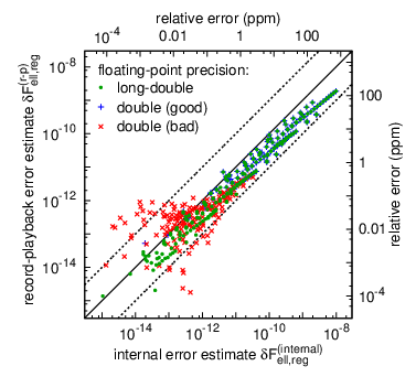
Figure 6 shows a scatterplot of the the record-playback error estimates versus the internal error estimates (32). The internal error estimates for evolutions done in long-double floating-point precision are generally generally consistent with the record-playback error estimates , and are somewhat conservative (the internal error estimates tend to overestimate the record-playback error estimates).
For evolutions done in double floating-point precision the internal error estimates are similarly consistent and conservative for the “good” parameters which are not shown as shaded in table 5 However, for the “bad” parameters which are shown as shaded in table 5 the internal error estimates scatter widely about the record-playback error estimates, often deviating by up to two orders of magnitude. This is due to floating-point rounding errors contaminating the numerical solution of the wave equation (9) (step 1 in the summary of section IV.8).
V.3.2 Self-Force Numerical Sum
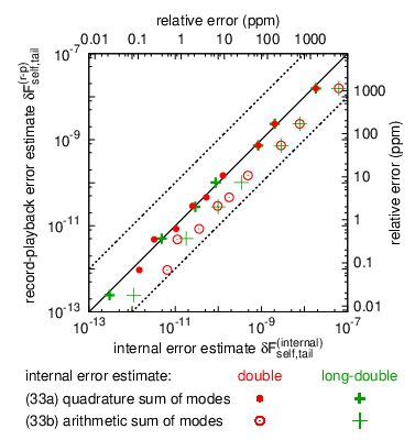
Figure 7 shows a scatterplot of the numerical-force record-playback error estimate versus the internal error estimate , the latter computed using each of the definitions (33). The arithmetic-sum internal error estimate (33b) systematically overestimates the record-playback error estimate by a factor of . In contrast, the quadrature-sum internal error estimate (33a) is quite accurate.2929 29 Notice that the set of modes considered here includes the “double (bad)” regularized self-force modes plotted in figure 6 and discussed in section V.3.1. Evidently the averaging inherent in summing 33 of these modes greatly reduces the effects of the floating-point roundoff error contamination of the individual modes. Based on this, I adopt the quadrature-sum internal error estimate (33a) hereinafter.
V.3.3 Self-Force Tail Sum
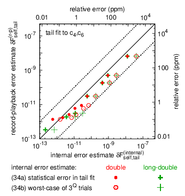
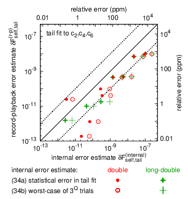
Figure 8 shows a scatterplot of the tail-force record-playback error estimate versus the internal error estimate (the latter computed using each combination of the definitions (34) and fitting either or ). When fitting (with given analytically by (25)), for both double and long-double floating-point precision the worst-case-of--trials internal error estimate (34b) tends to systematically overestimate the record-playback error estimate, while the statistical internal error estimate (34a) is much more accurate. Based on this, I adopt the statistical internal error estimate (34a) hereinafter. For both precisions, the internal error estimates change from being overestimates to underestimates of the record-playback error estimates for the two smallest-error points.
When fitting , the long-double internal error estimates are still consistent and somewhat conservative, but the three smallest-error internal error estimates scatter widely about the corresponding record-playback error estimates. This appears to be due to the ill-conditioning of the tail fit (cf. discussion in section IV.4, particularly table 4) amplifying the floating-point rounding errors in the individual regularized self-force modes .
I discuss further “quality control” checks based on the tail fits’ and residuals in section V.4.
V.3.4 Overall Self-Force
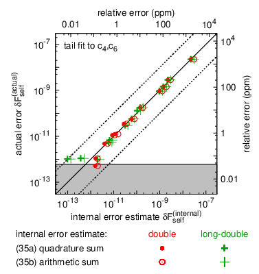
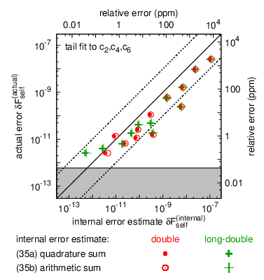
As discussed in section IV.7, I can compute the actual error of the overall self-force by comparing my calculations against previously published highly-accurate frequency-domain calculations. Figure 9 shows a scatterplot of the actual self-force errors versus the self-force internal error estimates (the latter computed using each combination of the definitions (35)) and for tail fits to or ). All of the error estimates are fairly accurate.
V.3.5 Record-Playback Error Estimates
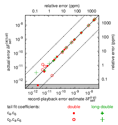
The self-force actual errors can also be used to validate the record-playback error estimates. Figure 10 shows a scatterplot of the actual self-force errors versus the record-playback error estimates . The actual errors are very similar to the record-playback error estimates.
V.4 The Tail Fits
The quality of a tail fit can be assessed via the fit’s : if lies outside the “plausible” range , where is the percentile of the distribution for the appropriate number of degrees of freedom (here for fitting , or for fitting ), we can reject the null hypothesis that the the nonzero fit residuals are solely due to (independent Gaussian-distributed) random errors of magnitudes given by the individual modes’ internal error estimates . A corollary of this is that the statistical tail-fit error estimate (34a) becomes unreliable.
Figure 11 shows the tail-fit for fitting both and for each set of numerical-accuracy parameters listed in table 5. For effective error tolerances the fits are very well-behaved: is small,3030 30 In fact, . This is due to the individual regularized self-force modes’ internal error estimates systematically overrestimating the actual numerical errors (cf. figure 6 and discussion in section V.3.1). and both the RMS residuals and the self-force actual errors decrease as decreases, as expected for a characteristic evolution scheme with 4th/6th order global/local finite differencing accuracy.
However, for the fits show several undesirable characteristics: increases, the RMS residuals either begin to increase with decreasing (double floating-point precision) or decrease at a slower rate than (long-double floating-point precision), and the actual errors either increase for the very smallest (double floating-point precision), level off as decreases (long-double floating-point precision, tail fit to only), or decrease at a slower rate than (long-double floating-point precision, tail fit to . These effects are due to floating-point roundoff errors contaminating the various steps of the calculation.

V.5 Cost/Accuracy Tradeoffs
There are a number of cost/accuracy tradeoffs inherent in the choice of the various numerical parameters in the self-force computation.
The computational cost is overwhelmingly dominated by the numerical solution of the wave equation (9) (step 1 in the summary of section IV.8), and is determined by the combination of the set of for which the wave equation (9) is solved, and the problem-domain sizes, floating-point precision, AMR error tolerances , and FMR refinement factors (if any) used in that solution.
In general, the problem-domain size should be chosen just large enough to render the errors induced by the remaining time dependence of small in comparison to other numerical errors. The problem-domain size required to ensure this varies with the magnitude of the other numerical errors, being larger for higher accuracies (smaller errors). The required problem-domain size also varies strongly with , being much larger for small (cf. discussion in section V.1). For simplicity, in this work I have only adjusted the problem-domain sizes at the very coarse level shown in table 6. A more careful adjustment would substantially improve the efficiency of the computation.
For my computational scheme, AMR and FMR are of almost equal efficiencies. That is, the grid structure, computational cost, and accuracy attained from an evolution using AMR with error tolerance and FMR by a refinement factor of are all very similar to those obtained from a purely-AMR evolution using the corresponding effective error tolerance . Assuming that the problem-domain sizes are large enough so that the remaining time dependence of isn’t a significant contributor to the overall error budget, the parameter space for cost-performance tradeoffs in numerically solving the wave equation (9) can thus be simplified to just the effective error tolerance .
The accuracy of a self-force computation is then determined by the combination of the set of for which the wave equation (9) is solved, the effective error tolerance of this solution, (the maximum included in the numerical force), the set of used in fitting the tail series (23), and the set of orders and corresponding coefficients included in this series. This is a large parameter space; for present purposes I restrict consideration to those parameter combinations listed in tables 5 and 7.
For present purposes, it’s useful to quantify the computational cost of an evolution by the total number of diamond cells integrated by the AMR algorithm. This is closely proportional to the overall CPU time used, with the constant of proportionality (the CPU time per diamond cell) being about () microseconds per diamond cell for double (long-double) floating-point precision on the processors used here. Figure 12 gives an overview of the cost-accuracy tradeoffs for the highest-accuracy set of numerical-force and tail-fit parameters shown in table 7 (i.e., those in in the last row of the table): the numerical force sums modes up to , the tail fit includes the modes , , and , and the tail fit fits either (with given analytically by (25)) or . It should be noted that the costs shown in this figure are for computations with very conservative (large) problem-domain sizes, and the wave equation (9) solve for a large set of . The costs could be greatly reduced with only a minor impact on the accuracy by using smaller problem-domain sizes and a smaller set of .

V.6 Results for the Self-Force
These results are fully consistent at the ppm level with the highly accurate frequency-domain results of Detweiler, Messaritaki, and Whiting [46]. Below ppm my results’ error estimates become increasingly unreliable due to floating-point roundoff errors, and below ppm the finite accuracy of the Detweiler, Messaritaki, and Whiting [46] results (their quoted error estimate is ppm) begins to affect comparisons with my results.
Tail fit fits coefficients ( is given analytically by the circular-orbit formula (25)):
| Floating-point | ||||||||||
| Precision | AMR/FMR | (11 d.o.f.) | absolute | relative | absolute | relative | absolute | relative | ||
| double | record | |||||||||
| double | playback2 | |||||||||
| double | record | |||||||||
| double | playback2 | |||||||||
| double | playback3 | |||||||||
| double | playback4 | |||||||||
| double | record | |||||||||
| double | playback2 | |||||||||
| double | playback3 | |||||||||
| double | playback4 | |||||||||
| double | playback6 | |||||||||
| [1.75][1.75]double | playback8 | |||||||||
| long-double | record | |||||||||
| long-double | playback2 | |||||||||
| long-double | record | |||||||||
| long-double | playback2 | |||||||||
| long-double | record | |||||||||
| long-double | playback2 | |||||||||
| long-double | record | |||||||||
| long-double | playback2 | |||||||||
| long-double | record | |||||||||
| long-double | playback2 | |||||||||
| long-double | record | |||||||||
| long-double | playback2 | |||||||||
| [1.75][1.75]long-double | playback23 | |||||||||
| Detweiler, Messaritaki, and Whiting | ||||||||||
Tail fit fits coefficients :
| Floating-point | ||||||||||
| Precision | AMR/FMR | (10 d.o.f.) | absolute | relative | absolute | relative | absolute | relative | ||
| double | record | |||||||||
| double | playback2 | |||||||||
| double | record | |||||||||
| double | playback2 | |||||||||
| double | playback3 | |||||||||
| double | playback4 | |||||||||
| double | record | |||||||||
| double | playback2 | |||||||||
| double | playback3 | |||||||||
| double | playback4 | |||||||||
| double | playback6 | |||||||||
| [1.75][1.75]double | playback8 | |||||||||
| long-double | record | |||||||||
| long-double | playback2 | |||||||||
| long-double | record | |||||||||
| long-double | playback2 | |||||||||
| long-double | record | |||||||||
| long-double | playback2 | |||||||||
| long-double | record | |||||||||
| long-double | playback2 | |||||||||
| long-double | record | |||||||||
| long-double | playback2 | |||||||||
| long-double | record | |||||||||
| long-double | playback2 | |||||||||
| long-double | playback23 | |||||||||
| Detweiler, Messaritaki, and Whiting | ||||||||||
VI Conclusions
This work demonstrates that the use of characteristic AMR can dramatically improve the efficiency of time-domain self-force calculations using the Barack-Ori mode-sum regularization formalism.3131 31 Cañizares and Sopuerta [62, 63] have used a multi-domain pseudospectral method to numerically solve the wave equation (9) within the same Barack-Ori mode-sum regularization framework as used here. Their results are quite promising, but are of relatively low accuracies (with typical relative errors of ) compared to the results reported here.
I find that the tail-fit basis is very ill-conditioned if many terms in the tail series (23) are fit simultaneously. Fortunately, normalizing the basis functions to have similar magnitudes mostly alleviates this ill-conditioning.
Past self-force calculations have often used “record-playback” error estimates derived from comparing a pair of different-resolution calculations. Here I present, and validate as quite reliable, a set of internal error estimators which can be used within a single self-force calculation (whether AMR or unigrid) to estimate the accuracy of individual regularized self-force modes , and the numerical force, tail force, and overall self-force derived from them.
In their pioneering calculation of the gravitational self-force acting on a mass particle on a circular geodesic orbit in Schwarzschild spacetime, Barack and Sago [54] use the arithmetic-sum formula (33b) to combine the numerical-force error given the (record-playback) error estimates of the individual modes. Here I show that (at least for my results) this formula is unnecessarily conservative, and that the quadrature-sum formula (33a) provides a better approximation to the numerical-force error over a wide range of overall computational accuracies.
Like other researchers (see, for example, [39, 54] and references therein, and the references cited in footnote 13), I find excellent agreement between time- and frequency-domain calculations of the self-force. Here I demonstrate this agreement down to the ppm accuracy level. Because the time- and frequency-domain calculations are structured so differently, this high-precision verification of their agreement provides a strong confirmation of the correctness of both calculations, and implicitly of their respective theoretical formalisms as well.
The present work could (should) be extended in several directions. Apart from the technical limits of the relatively coarse adjustment of the problem-domain size, one obvious extension would be to consider the electromagnetic and/or gravitational self-force. Another possibility would be to generalize the current finite differencing scheme to handle non-circular particle orbits. This would be straightforward, albeit somewhat tedious, using techniques such as those described by Haas [53] and Barack and Sago [54]. Once non-circular orbits can be handled, it should then be possible to move to full orbit-correction calculations of the type suggested by Gralla and Wald [34, section 7]. This will be very computationally demanding (it might benefit from further increasing the order of the finite differencing), but should provide valuable information about radiation-reaction effects.
The generalization of this work to particle orbits in Kerr spacetime would also be very valuable, but would demand a major reorganization of the mathematical and computational structure.
Acknowledgements.
I think Leor Barack for introducing me to the self-force problem, and Leor Barack, Norichika Sago, and Darren Golbourn for many valuable conversations and assistance with the self-force calculations. I thank Eric Ost for valuable assistance with the computer cluster used for many of the calculations described in this paper. I thank Michael Trosset, Stephanie Dickinson, and Lijiang Guo of Indiana University’s Indiana Statistical Consulting Center for their advice concerning the ill-conditioning and scaling of the tail fit.References
- [1] J. R. Gair, L. Barack, T. Creighton, C. Cutler, S. L. Larson, E. S. Phinney, and M. Vallisneri, Class. Quant. Grav., 21, S1595 (2004), gr-qc/0405137 .
- [2] L. Barack and C. Cutler, Phys. Rev. D, 69, 082005 (2004), gr-qc/0310125 .
- [3] P. Amaro-Seoane, J. R. Gair, M. Freitag, M. C. Miller, I. Mandel, C. J. Cutler, and S. Babak, Class. Quant. Grav., 24, R113 (2007), astro-ph/0703495 .
- [4] J. R. Gair, Class. Quant. Grav., 26, 094034 (2009), arXiv:0811.0188 .
- [5] T. Damour, in Three Hundred Years of Gravitation (Cambridge University Press, Cambridge, England, 1987) Chap. 6, pp. 128–198, ISBN 0-521-34312-7.
- [6] L. Blanchet, Living Reviews in Relativity, 9 (2006).
- [7] T. Futamase and Y. Itoh, Living Reviews in Relativity, 10 (2007).
- [8] L. Blanchet, in Mass and Motion in General Relativity, edited by L. Blanchet, A. Spallicci, and B. F. Whiting (Springer-Verlag, Berlin, 2010) ISBN 978-90-481-3014-6, arXiv:0907.3596 .
- [9] G. Schäfer, in Mass and Motion in General Relativity, edited by L. Blanchet, A. Spallicci, and B. F. Whiting (Springer-Verlag, Berlin, 2010) ISBN 978-90-481-3014-6, arXiv:0910.2857 .
- [10] F. Pretorius, in Relativistic Objects in Compact Binaries: From Birth to Coalescence, edited by M. Colpi (Springer-Verlag, 2007) arXiv:0710.1338 .
- [11] M. Hannam, S. Husa, J. G. Baker, M. Boyle, B. Brügmann, T. Chu, N. Dorband, F. Herrmann, I. Hinder, B. J. Kelly, L. E. Kidder, P. Laguna, K. D. Matthews, J. R. van Meter, H. P. Pfeiffer, D. Pollney, C. Reisswig, M. A. Scheel, and D. Shoemaker, Phys. Rev. D, 79, 084025 (2009), arXiv:0901.2437 .
- [12] M. Hannam, Class. Quant. Grav., 26, 114001 (2009), arXiv:0901.2931 .
- [13] M. Hannam and I. Hawke, “Numerical relativity simulations in the era of the Einstein telescope,” (2009), arXiv:0908.3139 .
- [14] M. Campanelli, C. O. Lousto, B. C. Mundim, H. Nakano, Y. Zlochower, and H.-P. Bischof, “Advances in simulations of generic black-hole binaries,” (2010), arXiv:1001.3834 .
- [15] N. T. Bishop, R. Gómez, S. Husa, L. Lehner, and J. Winicour, Phys. Rev. D, 68, 084015 (2003), gr-qc/0301060 .
- [16] N. T. Bishop, R. Gómez, L. Lehner, M. Maharaj, and J. Winicour, Phys. Rev. D, 72, 024002 (2005), gr-qc/0412080 .
- [17] C. F. Sopuerta, P. Sun, P. Laguna, and J. Xu, Class. Quant. Grav., 23, 251 (2006), gr-qc/0507112 .
- [18] C. F. Sopuerta and P. Laguna, Phys. Rev. D, 73, 044028 (2006), gr-qc/0512028 .
- [19] C. O. Lousto, H. Nakano, Y. Zlochower, and M. Campanelli, “Intermediate mass ratio black hole binaries: Numerical relativity meets perturbation theory,” (2010), arXiv:1001.2316 .
- [20] E. Poisson, Living Reviews in Relativity, 7 (2004).
- [21] S. Detweiler, Class. Quant. Grav., 22, S681 (2005).
- [22] L. M. Burko, Phys. Rev. D, 67, 084001 (2003).
- [23] L. M. Burko, Class. Quant. Grav., 22, S847 (2005).
- [24] E. Rosenthal, Class. Quant. Grav., 22, S859 (2005a), arXiv:0501046 .
- [25] E. Rosenthal, Phys. Rev. D, 72, 121503(R) (2005b), arXiv:0508050 .
- [26] E. Rosenthal, Phys. Rev. D, 73, 044034 (2006a), arXiv:0602066 .
- [27] E. Rosenthal, Phys. Rev. D, 74, 084018 (2006b), arXiv:0609069 .
- [28] B. S. DeWitt and R. W. Brehme, Annals of Physics, 9, 220 (1960).
- [29] J. M. Hobbs, Annals of Physics, 47, 141 (1968).
- [30] D. V. Gal’tsov, J. Phys. A, 15, 3737 (1982).
- [31] Y. Mino, M. Sasaki, and T. Tanaka, Phys. Rev. D, 55, 3457 (1997).
- [32] T. C. Quinn and R. M. Wald, Phys. Rev. D, 56, 3381 (1997), gr-qc/9610053 .
- [33] S. Detweiler, Phys. Rev. Lett., 86, 1931 (2001), gr-qc/0011039 .
- [34] S. E. Gralla and R. M. Wald, Class. Quant. Grav., 25, 205009 (2008).
- [35] S. E. Gralla, A. I. Harte, and R. M. Wald, Phys. Rev. D, 80, 024031 (2009).
- [36] L. Barack, Class. Quant. Grav., 26, 213001 (2009), arXiv:0908.1664 .
- [37] S. Detweiler, in Mass and Motion in General Relativity, edited by L. Blanchet, A. Spallicci, and B. F. Whiting (Springer-Verlag, Berlin, 2010) ISBN 978-90-481-3014-6, arXiv:0908.4363 .
- [38] E. Poisson, in Mass and Motion in General Relativity, edited by L. Blanchet, A. Spallicci, and B. F. Whiting (Springer-Verlag, Berlin, 2010) ISBN 978-90-481-3014-6, arXiv:0909.2994 .
- [39] N. Sago, L. Barack, and S. Detweiler, Phys. Rev. D, 78, 124024 (2008), arXiv:0810.2530 .
- [40] L. Barack and A. Ori, Phys. Rev. D, 61, 061502 (2000), gr-qc/9912010 .
- [41] L. Barack, Phys. Rev. D, 62, 084027 (2000), gr-qc/0005042 .
- [42] L. Barack, Y. Mino, H. Nakano, A. Ori, , and M. Sasaki, Phys. Rev. Lett., 88, 091101 (2002), gr-qc/0111001 .
- [43] L. Barack and A. Ori, Phys. Rev. D, 66, 084022 (2002), gr-qc/0204093 .
- [44] L. Barack and A. Ori, Phys. Rev. D, 67, 024029 (2003), gr-qc/0209072 .
- [45] S. Detweiler and B. F. Whiting, Phys. Rev. D, 67, 024025 (2003).
- [46] S. Detweiler, E. Messaritaki, and B. F. Whiting, Phys. Rev. D, 67, 104016 (2003).
- [47] R. Haas and E. Poisson, Phys. Rev. D, 74, 044009 (2006).
- [48] L. Blanchet, S. Detweiler, A. Le Tiec, and B. F. Whiting, “Post-Newtonian and numerical calculations of the gravitational self-force for circular orbits in the Schwarzschild geometry,” (2009), arXiv:0910.0207 .
- [49] K. Glampedakis and D. Kennefick, Phys. Rev. D, 66, 044002 (2002).
- [50] L. Barack and C. O. Lousto, Phys. Rev. D, 72, 104026 (2005), gr-qc/0510019 .
- [51] L. Barack, A. Ori, and N. Sago, Phys. Rev. D, 78, 084021 (2008), arXiv:0808.2315 .
- [52] J. L. Barton, D. J. Lazar, D. J. Kennefick, G. Khanna, and L. M. Burko, Phys. Rev. D, 78, 064042 (2008), arXiv:0804.1075 .
- [53] R. Haas, Phys. Rev. D, 75, 124011 (2007), arXiv:0704.0797 .
- [54] L. Barack and N. Sago, Phys. Rev. D, 81, 084021 (2010), arXiv:1002.2386 .
- [55] J. Thornburg, “Berger-Oliger mesh refinement for characteristic grids,” (2009), arXiv:0909.0036 .
- [56] L. Barack and L. M. Burko, Phys. Rev. D, 62, 084040 (2000), gr-qc/0007033 .
- [57] L. M. Burko, Class. Quant. Grav., 17, 227 (2000a).
- [58] L. M. Burko, Phys. Rev. Lett., 84, 4529 (2000b).
- [59] L. M. Diaz-Rivera, E. Messaritaki, B. F. Whiting, and S. Detweiler, Phys. Rev. D, 70, 124018 (2004).
- [60] I. Vega and S. Detweiler, Phys. Rev. D, 77, 084008 (2008), arXiv:0712.4405 .
- [61] I. Vega, P. Diener, W. Tichy, and S. Detweiler, Phys. Rev. D, 80, 084021 (2009), arXiv:0908.2138 .
- [62] P. Cañizares and C. F. Sopuerta, J. Physics: Conference Series, 159, 012053 (2009a), proceedings of the 7th International LISA Symposium, Barcelona, Spain, 16–20 June 2008, arXiv:0811.0294 .
- [63] P. Cañizares and C. F. Sopuerta, Phys. Rev. D, 79, 084020 (2009b), arXiv:0903.0505 .
- [64] T. S. Keidl, J. L. Friedman, and A. G. Wiseman, Phys. Rev. D, 75, 124009 (2007), gr-qc/0611072 .
- [65] L. Barack and C. O. Lousto, Phys. Rev. D, 66, 061502(R) (2002), gr-qc/0205043 .
- [66] L. Barack and N. Sago, Phys. Rev. D, 75, 064021 (2007), gr-qc/0701069 .
- [67] L. Barack and N. Sago, Phys. Rev. Lett., 102, 191101 (2009), arXiv:0902.0573 .
- [68] S. Detweiler, Phys. Rev. D, 77, 124026 (2008).
- [69] N. Warburton and L. Barack, Phys. Rev. D, 81, 084039 (2010), arXiv:1003.1860 .
- [70] R. M. Wald, General relativity, Wald84 (The University of Chicago Press, Chicago, 1984) ISBN 0-226-87032-4 (hardcover), 0-226-87033-2 (paperback).
- [71] E. K. Porter, “An overview of LISA data analysis algorithms,” (2009), arXiv:0910.0373 .
- [72] F. D. Ryan, Phys. Rev. D, 52, 5707 (1995).
- [73] F. D. Ryan, Phys. Rev. D, 56, 1845 (1997).
- [74] C. Hopman (American Institute of Physics, 2006) pp. 241–249, astro-ph/0608460 .
- [75] K. Glampedakis and S. Babak, Class. Quant. Grav., 23, 4167 (2006).
- [76] L. Barack and C. Cutler, Phys. Rev. D, 75, 042003 (2007), gr-qc/0612029 .
- [77] M. C. Miller, T. Alexander, P. Amaro-Seoane, A. J. Barth, C. Cutler, J. R. Gair, C. Hopman, D. Merritt, E. S. Phinney, and D. O. Richstone, “Probing stellar dynamics in galactic nuclei,” (2009), arXiv:0903.0285 .
- [78] G. Malmquist, Medd. Lund Astron. Obs., Ser. II, 22, 1 (1920), (Author is often cited as K. G. Malmquist.).
- [79] P. Teerikorpi, Annual Rev. Astron. Astrophys., 35, 101 (1997).
- [80] D. Psaltis, Living Reviews in Relativity, 11 (2008).
- [81] S. J. Vigeland and S. A. Hughes, Phys. Rev. D, 81, 024030 (2010), arXiv:0911.1756 .
- [82] L. S. Finn, Phys. Rev. D, 46, 5236 (1992).
- [83] C. Cutler and E. E. Flanagan, Phys. Rev. D, 49, 2658 (1994).
- [84] A. K. Piotr Jaranowski, Living Reviews in Relativity, 8 (2005).
- [85] C. Cutler and M. Vallisneri, Phys. Rev. D, 76, 104018 (2007).
- [86] M. Vallisneri, Phys. Rev. D, 77, 042001 (2008), gr-qc/0703086 .
- [87] E. A. Huerta and J. R. Gair, Phys. Rev. D, 79, 084021 (2009).
- [88] L. Lindblom, B. J. Owen, and D. A. Brown, Phys. Rev. D, 78, 124020 (2008).
- [89] L. Lindblom, Phys. Rev. D, 80, 042005 (2009a).
- [90] L. Lindblom, Phys. Rev. D, 80, 064019 (2009b).
- [91] T. Damour, “Gravitational self force in a Schwarzschild background and the effective one body formalism,” (2009), arXiv:0910.5533 .
- [92] C. W. Gear, SIAM Review, 23, 10 (1981).
- [93] S. E. Field, J. S. Hesthaven, and S. R. Lau, “Persistent junk solutions in time-domain modeling of extreme mass ratio binaries,” (2010), arXiv:1001.2578 .
- [94] B. Char, K. O. Geddes, W. M. Gentleman, and G. H. Gonnet, in Lecture Notes in Computer Science 162: Computer Algebra, edited by J. A. van Hulzen (Springer-Verlag, 1983) pp. 101–115.
- [95] R. Gómez and J. Winicour, J. Math. Physics, 33, 1445 (1992).
- [96] R. Gómez, J. Winicour, and R. Isaacson, J. Comp. Phys., 98, 11 (1992).
- [97] C. Gundlach, R. Price, and J. Pullin, Phys. Rev. D, 49, 883 (1994), gr-qc/9307009 .
- [98] L. M. Burko and A. Ori, Phys. Rev. D, 56, 7820 (1997).
- [99] C. O. Lousto and R. H. Price, Phys. Rev. D, 56, 6439 (1997), gr-qc/9705071 .
- [100] C. O. Lousto, Class. Quant. Grav., 22, S543 (2005).
- [101] J. Winicour, Living Reviews in Relativity, 12 (2009).
- [102] M. J. Berger and J. Oliger, J. Comput. Phys., 53, 484 (1984).
- [103] M. J. Berger, Adaptive Mesh Refinement for Hyperbolic Partial Differential Equations, Ph.D. thesis, Stanford University (1982), University Microfilms #DA 83-01196.
- [104] M. J. Berger, SIAM Journal of Scientific and Statistical Computing, 7, 904 (1986).
- [105] M. J. Berger and P. Colella, J. Comput. Phys., 82, 64 (1989).
- [106] M. W. Choptuik, in Frontiers in Numerical Relativity, edited by C. Evans, L. Finn, and D. Hobill (Cambridge University Press, Cambridge, England, 1989) pp. 206–221.
- [107] M. W. Choptuik, in Approaches to Numerical Relativity, edited by R. d’Inverno (Cambridge University Press, Cambridge, 1992) pp. 202–222.
- [108] R. S. Hamadé and J. M. Stewart, Class. Quant. Grav., 13, 497 (1996), gr-qc/9506044 .
- [109] H. O. Kreiss and J. Oliger, Methods for the approximate solution of time dependent problems (GARP publication series No. 10, Geneva, 1973).
- [110] M. W. Choptuik, Phys. Rev. D, 44, 3124 (1991).
- [111] R. D. Richtmyer and K. Morton, Difference Methods for Initial Value Problems, 2nd ed. (Kreiger, Malabar, Florida, USA, 1994) ISBN 0-89464-763-6.
- [112] R. J. LeVeque, Finite Difference Methods for Ordinary and Partial Differential Equations (SIAM Press, Philadelphia, USA, 2007) ISBN 978-0-898716-29-0.
- [113] G. E. Forsythe, M. A. Malcolm, and C. B. Moler, Computer Methods for Mathematical Computations (Prentice-Hall, Englewood Cliffs, 1977) ISBN 0-13-165332-6, software available at http://www.netlib.org/fmm/.
- [114] D. Kahaner, C. B. Moler, and S. Nash, Numerical Methods and Software (Prentice-Hall, Englewood Cliffs, 1989) ISBN 0-13-627258-4.
- [115] D. Goldberg, ACM Computing Surveys, 23, 5 (1991).
- [116] W. Kahan, Communications of the ACM, 8, 40 (1965).
- [117] S. L. B. Moshier, Methods and Programs for Mathematical Functions (Ellis Horwood, Chichester, U.K., 1989) ISBN 978-0-13578-998-8.
- [118] R. Piessens, E. de Doncker-Kapenga, C. W. Überhuber, and D. Kahaner, Quadpack: A subroutine package for automatic integration (Springer-Verlag, Berlin, 1983) ISBN 3-540-12553-1.
- [119] C. L. Lawson and R. J. Hanson, Solving Least Squares Problems (Prentice-Hall, Englewood Cliffs, New Jersey, 1974) ISBN 0-13-822585-0.
- [120] S. Hammarling, ACM SIGNUM Newsletter, 20, 2 (1985).
- [121] W. H. Press, S. A. Teukolsky, W. T. Vetterling, and B. P. Flannery, Numerical Recipes in Fortran 77, 2nd ed. (Cambridge University Press, 1992) ISBN 0-521-43064-X.
- [122] Å. Björck, Numerical Methods for Least Squares Problems (SIAM Press, Philadelphia, USA, 1996) ISBN 978-0-898713-60-2.
- [123] M. Galassi, J. Davies, J. Theiler, B. Gough, G. Jungman, P. Alken, M. Booth, and F. Rossi, GNU Scientific Library Reference Manual, 3rd ed. (Network Theory Ltd., 2009) ISBN 978-0-9546120-7-8.