Solitary waves of Bose-Einstein condensed atoms confined in finite rings
Abstract
Motivated by recent progress in trapping Bose-Einstein condensed atoms in toroidal potentials, we examine solitary-wave solutions of the nonlinear Schrödinger equation subject to periodic boundary conditions. When the circumference of the ring is much larger than the size of the wave, the density profile is well approximated by that of an infinite ring, however the density and the velocity of propagation cannot vanish simultaneously. When the size of the ring becomes comparable to the size of the wave, the density variation becomes sinusoidal and the velocity of propagation saturates to a constant value.
pacs
05.30.Jp, 67.85.Hj, 67.85.JkI Introduction
The problem of solitary-wave solutions of the one-dimensional nonlinear Schrödinger equation has been studied extensively, starting with the work of Zakharov and Shabat [1] and of Tsuzuki [2]. In addition, Lieb [3] has examined the problem of a Bose gas in strictly one dimension with periodic boundary conditions and a repulsive interaction, and he derived the excitation spectrum. As demonstrated in that study, the spectrum consists of the usual Bogoliubov branch as well as a second branch. This branch was later identified as corresponding to solitary-wave excitation [4, 5].
Bose-Einstein condensed atoms interacting via a contact potential are described by a nonlinear Schrödinger equation and thus offer a very suitable system for the study of solitary waves [6]. Solitary waves have been created in quasi-one-dimensional traps with a very weak harmonic potential in the long direction [7] and in pancake traps [8]. Recently, it also became possible to confine atoms in toroidal traps [9, 10, 11, 12, 13] in which persistent currents were observed [13].
Based on this experimental progress, it is natural to consider the possible creation of solitary waves in such toroidal traps. This is the subject of the present study. In the following, we examine the properties of solitary waves, including their density, propagation velocity, and phase (and thus the superfluid velocity), with periodic boundary conditions. We note that Carr et al. [14] have previously considered the special case of static periodic solitary-wave solutions for a fixed particle number and a length.
For simplicity we consider in the present study a very tight toroidal trap, neglecting the transverse degrees of freedom, and thus consider the purely one-dimensional motion of atoms on a ring. The main question to be considered here is the behavior of solitonic solutions as the length of the period is varied for fixed , where is the number of particles. The relevant dimensionless parameter is the ratio of and the coherence length, , which we choose as that corresponding to the maximum density. According to the value of we distinguish between “large” rings, where , and “small” rings, where . In Lieb’s study [3], the limit and with finite was considered. This corresponds to the limit of large rings in the present study. We note that the ratio also describes the ratio between the typical zero-point energy, , and the typical interaction energy, . Finally, we restrict ourselves to the case of repulsive effective interatomic interactions.
As we will show below, in the limit of large rings, the wave is localized within a length scale determined by the coherence length, and the density is constant over the rest of the system, in agreement with known results for an infinite system. On the other hand, depending on the phase difference at the edges of the system (which is either zero or some integer multiple of ), two different situations can arise. For zero phase difference, the minimum possible value of the density is zero, and the velocity of propagation varies between a lowest nonzero value, which scales as and essentially corresponds to the superfluid “drift” velocity, and a maximum velocity which is set by the speed of sound. In the case of a nonzero phase difference, the velocity of propagation can be zero, but the corresponding density cannot vanish, scaling like . Clearly, when and with finite, we find agreement with known results.
In the opposite limit of small rings, the density becomes sinusoidal with a length scale given by itself. Furthermore, the velocity of propagation saturates to a constant value, which scales like , and the minimum density can become zero.
In what follows we first formulate our problem in Sec. II. Then, in Sec. III we give the general solution. Section IV examines certain limiting cases, starting from the linearization of the problem and then turning to the limits of large and small rings. In Sec. V we present a general result for the minimum value of the velocity of propagation of the wave, and finally we summarize our results and present our conclusions in Sec. VI.
II Formulation of the problem
Assume that we have a ring of circumference which contains atoms of mass . Within the mean-field approximation, the order parameter satisfies the equation (in the range ),
| (1) |
with and , because of the repulsive interatomic interactions that we consider. Assuming that , where is the chemical potential and ,
| (2) |
Here is the velocity of propagation of the assumed traveling-wave solution. Setting , the superfluid velocity is given by the continuity equation
| (3) |
There is also an Euler equation for the density,
| (4) |
where and are constants of integration.
The desired solution has a vanishing derivative at the points and where and , respectively. This allows us to eliminate from Eq. (4) and to determine that
| (5) |
This leads to
| (6) |
with . In the case of an infinite system, and , in which case Eq. (6) then reduces to the correct and known form of the differential equation.
III The general solution
The general solution of Eq. (6) which is periodic in the interval between and is [14]
| (7) | |||||
where and are Jacobi elliptic functions and is the elliptic integral of the first kind. Since and , we see that and . In order for Eq. (7) to be the solution of the differential equation of Eq. (6),
| (8) |
where is the coherence length corresponding to a density , , and . Similarly, and are given as
| (9) |
and
| (10) |
Since as and as , ranges between 0 and 1. Clearly the solution of Eq. (7) can be immediately extended to describe identical solitary waves on a ring of circumference .
The velocity of propagation, , can then be determined by integrating the continuity equation, Eq. (3), over one period,
| (11) | |||||
Assuming that with an integer as a consequence of the periodic boundary conditions, we solve the above equation in terms of and combine it with Eq. (5) to obtain
| (12) |
Here is the speed of sound of a homogeneous gas of density , . We remark from Eq. (11) that and have opposite signs when .
While the parameterization of that we adopt above is natural mathematically, it is of greater physical interest to explore solutions for fixed , , and as a function of, e.g., . To this end, it is convenient to pick a value of and , and determine from Eq. (8). It is clear from its definition that must be greater than or equal to zero for physically meaningful solutions. The value of can then be adjusted to satisfy the normalization condition on .
Equations (7), (8), and (12) are consistent with Bloch’s theorem [15]. Because of the periodic boundary conditions imposed, the order parameter of the solitary wave corresponding to the branch with quantum number is given by that obtained for by exciting the center of mass motion, . These two solutions have the same density, but there is a difference in the velocity of propagation so that , in agreement with Eq. (12). Similarly, the energy spectrum consists of a periodic part plus an envelope function which results from the energy of the center of mass motion.
IV Limiting cases
IV.1 Linearization of the problem
When , one can obtain equations for the force and for continuity by linearizing the problem in small deviations of the density and the phase from the homogeneous solution ,
| (13) |
where and . When the two are combined, we obtain
| (14) |
Thus, with and constants. Periodicity requires that with an integer. Here, we set so that
| (15) |
In the limit of “large” rings, i.e., ,
| (16) |
In the opposite limit of “small” rings, , then
| (17) |
We note that Eq. (15) can also be derived directly from Eq. (12) provided that one considers a fixed length and then takes , which implies that in Eqs. (7) and (8).
IV.2 Limit of large rings
We now consider the limiting forms of the solution appropriate for large and small rings. For large rings, , and the general solution of Eq. (7) reduces to
| (18) |
where . This is in agreement with the known result, plus corrections of order . In this limit, with
| (19) |
and also . From Eq. (12) we find that
| (20) | |||||
which reduces to the familiar result in the limit of an infinite ring.
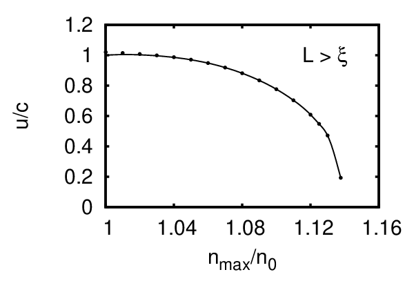
Figure 1 shows as a function of for the parameter choice , , , and (with ) so that . Exact results (dots) derived from Eq. (11), and values obtained using the approximation of Eq. (20) are given. The agreement is remarkably good except in the limit . In this limit, Eq. (20) yields , which does not contain the higher-order quadratic term seen in Eq. (16). In the opposite limit, where , Eq. (20) gives the exact result, as shown in Sec. V.
In the limit of small Eq. (20) reduces to
| (21) |
Consider first the choice . In this case can be arbitrarily small in analogy with a “dark” solitary wave in the limit. The velocity of propagation is bounded from below by , , which corresponds to the minimum value of shown in Fig. 1. Equivalently,
| (22) |
except in the immediate vicinity of the solitary wave. This result is easily understood. As Eqs. (3) and (10) imply, when , and the superfluid velocity is independent of position and equal to the velocity of propagation . In the limit of a dark solitary wave, the phase varies linearly, except in the limited region of small density, where the phase develops a discontinuity of . In order to satisfy the condition , must have the small slope over a large length . Thus, as Eq. (22) indicates, cannot be zero.
In the case , can vanish, but when vanishes, is
| (23) |
This result is also easy to understand. Let us set . In this case Eq. (3) implies that . Away from the center of the wave, is constant and equal to since the density is constant, but the phase is equal to . The total accumulation of the phase over is thus approximately , while another is needed in order to create the total phase difference of . This is provided from the region around the wave where , within a length scale of order . This is the length scale of the dominant integration interval of around its singularity. Since is in this regime, and in order for the integral of to be equal to when we integrate it around a length scale of order , we find that
| (24) |
This implies that .
These results agree with those of Carr et al. [14]. In that study only static solitary waves were considered, and (as mentioned in Ref. [14]) this is not possible for zero phase difference. Their choice of leads to according to Eq. (23), which is in good agreement with the numerical results of Fig. 4 of this reference.
It should also be noted that Eq. (23) is valid for a single solitary-wave solution. For a two-solitary wave solution it is possible for them to be both static and dark (i.e., to have a node in the density).
The maximum possible value of is achieved in the limit of sound waves where
| (25) |
in agreement with Eq. (16). Finally, we note that the normalization condition takes the form in this limit.

IV.3 Limit of small rings
For small rings, , the general solution of Eq. (7) reduces to
| (26) |
plus corrections of order (i.e., of order ) since and in the limit . Turning to the velocity of propagation of the wave, Eq. (12) implies that in the limit of small rings
| (27) |
One can identify the term proportional to as the difference , where is the single-particle kinetic energy of a particle in a ring of radius with angular momentum , and . This expression coincides with Eq. (17), found by linearization, when and . Here, is not bounded from below as it was in the limit of large rings. Remarkably, saturates to a constant value independent of when . This happens because
| (28) | |||||
in this limit, since the integral is independent of . In other words, in the limit of small rings, the sinusoidal dependence of the density always gives rise to a phase difference of for any value of the ratio . Since the periodic boundary conditions require that the total phase difference has to be , the additional phase accumulation must be . This fact gives a slope to the phase that is (plus corrections of order , and therefore , in agreement with Eq. (28). Finally, the normalization condition is in this limit.
Figure 2 shows as a function of for the parameter choice , , , and (with ), so that . Exact results (dots) and values obtained using the approximation of Eq. (27) are given. The agreement is remarkably good in both limits , and , as Eq. (27) gives the exact result in both cases, as Eqs. (17) and (29) indicate.
V A general result
It is interesting to note that, in the limit of a dark solitary wave (), the velocity of propagation of the wave is given by the same formula,
| (29) |
or
| (30) |
in the limits of both small and large rings, as indicated by Eqs. (21) and (27). In fact, Eq. (29) gives the minimum possible value of for any : A change of variable tranforms Eq. (12) into
| (31) |
The integral can be evaluated in the limit by closing the integration contour with a semicircle in the upper half complex plane. The only contribution to the integral comes from the pole at . In this way, one obtains Eq. (29) for any finite value of .
In the limit where , the integral in Eq. (12) is dominated by the behavior of the density near since for . As a result, the integral is approximately proportional to . As a result, there is a contribution to which is equal to . For a nonzero , there is an additional contribution of to , from which Eqs. (29) and (30) follow.
VI Summary and conclusions
To summarize, solitary-wave solutions of the nonlinear Schrödinger equation framework show interesting features if one imposes the periodic boundary conditions appropriate for the description of Bose-Einstein condensed atoms confined in tight toroidal traps.
In the limit of large rings, where the size of the wave is much smaller than the length of the ring, the density is exponentially localized on a length scale determined by the coherence length and is constant over the remainder of the ring. Depending on the phase difference at the edges of the period, either the minimum density can vanish (with the velocity of propagation being nonzero) or the velocity of propagation can vanish (with the minimum density being nonzero). However, both cannot be zero simultaneously.
In the limit of small rings, the density is sinusoidal within a length scale given by the circumference of the ring itself. The velocity of propagation saturates to a constant value, which is independent of . For this reason, the size of the ring must exceed some minimum size in order to create a static wave with [14]. The minimum size can be determined from Eq. (31) for and in the limit and with . Under these conditions, and , in agreement with Ref. [14].
In the limit of an infinite ring, the velocity of propagation of the solitary wave depends on the ratio . In the opposite limit of small rings, the range of possible values of the velocity of propagation becomes narrower as decreases. In the limit of very small , saturates to a constant value and becomes independent of .
The general result that the minimum value of is inversely proportional to may be relatively easy to investigate experimentally.
Finally, we note that as opposed to the case of an infinite ring, which contains only the dimensionless quantity , a second dimensionless quantity, , appears in the present problem. In particular, in the limit of sound waves (where ) and large rings (where ), the product of these two terms appears, and the two limits “compete”. Different answers will result depending on the way in which these limits are taken. These different answers are not only of theoretical interest; they represent different physical situations determined by the way that an experiment is performed.
Acknowledgements.
We thank N. Efremidis, W. von Klitzing, and S. Komineas for useful discussions.References
- [1] V. E. Zakharov and A. B. Shabat, Zh. Eksp. Teor. Fiz. 64, 1627 (1973) [Sov. Phys. JETP 37, 823 (1973)].
- [2] T. Tsuzuki, J. Low Temp. Phys. 4, 441 (1971).
- [3] E. Lieb, Phys. Rev. 130, 1616 (1963).
- [4] P. P. Kulish, S. V. Manakov, and L. D. Faddeev, Theor. Math. Phy. 28, 615 (1976).
- [5] M. Ishikawa and H. Takayama, J. Phys. Soc. Jpn. 49, 1242 (1980).
- [6] D. J. Frantzeskakis, J. Phys. A: Math. Theor. 43, 213001 (2010).
- [7] S. Burger, K. Bongs, S. Dettmer, W. Ertmer, K. Sengstock, A. Sanpera, G. V. Shlyapnikov, and M. Lewenstein, Phys. Rev. Lett. 83, 5198 (1999)
- [8] J. Denschlag, J. E. Simsarian, D. L. Feder, C. W. Clark, L. A. Collins, J. Cubizolles, L. Deng, E. W. Hagley, K. Helmerson, W. P. Reinhardt, S. L. Rolston, B. I. Schneider, and W. D. Phillips, Science 287, 97 (2000).
- [9] S. Gupta, K. W. Murch, K. L. Moore, T. P. Purdy, and D. M. Stamper-Kurn, Phys. Rev. Lett. 95, 143201 (2005).
- [10] S. E. Olson, M. L. Terraciano, M. Bashkansky, and F. K. Fatemi, Phys. Rev. A 76, 061404(R) (2007).
- [11] I. Lesanovsky and W. von Klitzing, Phys. Rev. Lett. 99, 083001 (2007).
- [12] K. Henderson, C. Ryu, C. MacCormick, and M. G. Boshier, New J. Phys. 11, 043030 (2009).
- [13] C. Ryu, M. F. Andersen, P. Cladé, V. Natarajan, K. Helmerson, and W. D. Phillips, Phys. Rev. Lett. 99, 260401 (2007).
- [14] L. D. Carr, C. W. Clark, and W. P. Reinhardt, Phys. Rev. A 62, 063610 (2000).
- [15] F. Bloch, Phys. Rev. A 7, 2187 (1973).