Bloch Solutions of Periodic Dirac Equations in SPPS Form

The connections between the Dirac equation and the Schrödinger equation are known since a long time ago [4] and have been strengthen in the supersymmetric context soon after the advent of supersymmetric quantum mechanics in 1981 [5, 6, 7, 8]. There are currently interesting applications of this approach in condensed matter physics [9, 10, 11]. In this work, we are interested in the same connection in the case of periodic potentials, see e.g. [12]. We here write the Dirac Bloch solutions in Kravchenko form (power series in the spectral parameter) and also the Dirac Hill discriminant in the same form and apply the results to an interesting quasi-exactly solvable periodic potential.

The Schrödinger differential equation

with $T$-periodic real-valued potential $q(x)$ assumed herewith a continuous bounded function and $\lambda$ a real parameter is known as of Hill type. We begin by recalling some necessary definitions and basic properties associated with the equation (1) from the Floquet (Bloch) theory. For more details see, e.g., [13, 14].

For each $\lambda$ there exists a fundamental system of solutions, i.e., two linearly independent solutions of (1), $f_{1}(x,\lambda)$ and $f_{2}(x,\lambda)$, which satisfy the initial conditions

Then the Hill discriminant associated with equation (1) is defined as a function of $\lambda$ as follows

The importance of $D(\lambda)$ stems from the easiness of describing the spectrum of the corresponding equation by its means, namely [13]:

(1) sets $\{\lambda_{i}\}$ for which $\left|D(\lambda)\right|\leq 2$ form the allowed bands or stability intervals,
(2) sets $\{\lambda_{j}\}$ for which $\left|D(\lambda)\right|>2$ form the forbidden bands or instability intervals,
(3) sets $\{\lambda_{k}\}$ for which $\left|D(\lambda)\right|=2$ form the band edges and represent the discrete part of the spectrum.

We consider the following Dirac equation

where the scalar potential $\Phi(x)$ is periodic function with period $T$, $W$ is the spinor $W=\left(\begin{array}[c]{c}f\\ g\end{array}\right)$ and $\sigma_{x}$, $\sigma_{y}$ are the Pauli matrices $\sigma_{x}=\left(\begin{array}[c]{cc}0&1\\ 1&0\end{array}\right)$ and $\sigma_{y}=\left(\begin{array}[c]{cc}0&-i\\ i&0\end{array}\right).$

The uncoupled Schrödinger equations derived from equation (5) are

where $\lambda=\omega^{2}$ is the spectral parameter. It is clear that the solutions $f$ and $g$ are related by the following relationship

therefore with the solution $f$ at hand, we can construct the solution $g$ immediately.

We start with equation (6). Notice that the solution $u$ of the equation (6) for $\lambda=0$ can be obtained as follows $u(x)=e^{-\int\Phi(x)dx}$ and $u(x)$ is a nodeless periodic function with the period $T$ if $\Phi(x)\in\mathbf{C}^{1}$ and $\int_{0}^{T}\Phi(x)dx=0$.

Once having the function $u(x)$ the solutions $f_{1}(x,\lambda)$ and $f_{2}(x,\lambda)$ of (6), (2) for all values of the parameter $\lambda$ can be given using the SPPS method [1] .

The functions $\widetilde{\Sigma}_{0}$ and $\Sigma_{1}$ are the spectral parameter power series

where the coefficients $\widetilde{X}^{(n)}(x)$, $X^{(n)}(x)$ are given by the following recursive relations

One can check by a straightforward calculation that the solutions $f_{1}$ and $f_{2}$ fulfill the initial conditions (2), for this the following relations are useful

and

The pair of linearly independent solutions $g_{1}(x,\lambda)$ and $g_{2}(x,\lambda)$ of (7) can be obtained directly from the solutions (9) by means of (8). We additionally take the linear combinations in order that the solutions $g_{1}(x,\lambda)$ and $g_{2}(x,\lambda)$ satisfy the initial conditions $g_{1}(0,\lambda)=g_{2}^{\prime}(0,\lambda)=1$ and $g_{1}^{\prime}(0,\lambda)=g_{2}(0,\lambda)=0$

Thus, the two spinor solutions of the Dirac equation (5) are given by

and these solutions satisfy the following initial conditions

As is well known [13], the zeros of the functions $D(\lambda)\mp 2$ represent eigenvalues of the corresponding Hill operator with periodic and aperiodic boundary conditions, respectively. In this section, we show that besides other possible applications the representation (15) gives us an efficient tool for the calculation of the discrete spectrum of a periodic Dirac operator.

The first step of the numerical realization of the method consists in calculation of the functions $\tilde{X}^{(n)}$ and $X^{(n)}$ given by (10) and (11), respectively. This construction is based on the eigenfunction $u(x)$. Next, by truncating the infinite series for $D(\lambda)$ (15) we obtain a polynomial in $\lambda$

The roots of the polynomials $D_{N}(\lambda)\mp 2$ give us the eigenvalues corresponding to equation (1) with periodic and aperiodic boundary conditions, respectively.

As an example we consider the Dirac equation (5) with the scalar potential

with $A(\xi)=\left(1-\sqrt{1+\xi^{2}}\right)$ and $\xi$ a real positive parameter. This scalar potential satisfies the conditions of theorem 3.1. The corresponding second order differential equations are

where the Schrödinger potential

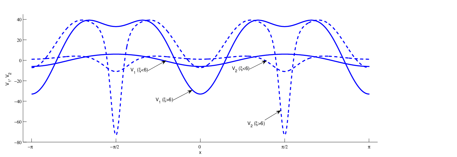
is the case $m=2$ in the quasi-exactly solvable family of the so-called trigonometric Razavy potentials [17], $V_{R}=\frac{\xi^{2}}{8}\left(1-\cos 4x\right)-(m+1)\xi\cos 2x$. For a given integer $m$, if $\xi<2(m+1)$ the potentials $V_{R}(x)$ are of single-well periodic type and if $\xi>2(m+1)$ they are of double-well periodic type.

is the supersymmetric partner potential and therefore it is also quasi-exactly solvable. The Schrödinger equations with these potentials can be used for the description of torsional oscillations of certain molecules [17]. Plots of the potentials $V_{1}(x)$ and $V_{2}(x)$ are displayed in Fig. 1 for two values of $\xi$.

The computer algorithm was implemented in Matlab 2006. The recursive integration required for the construction of $\tilde{X}_{0}^{(n)}$, $X_{0}^{(n)}$, $\tilde{X}^{(n)}$ and $X^{(n)}$ was done by representing the integrand through a cubic spline using the $\emph{spapi}$ routine with a division of the interval $[0,\pi]$ into $5000$ subintervals and integrating using the $\emph{fnint}$ routine. Next, the zeros of $D_{N}(\lambda)\pm 2$ were calculated by means of the $\emph{fnzeros}$ routine.

In the following tables, the eigenvalues were calculated employing the SPPS representation (15) for four different values of the parameter $\xi$. The first two values are below the threshold value $\xi_{\rm thr}=6$ for $m=2$ from single-well to double-well types of Razavy’s potentials while the last two values are above this threshold value. For comparison, we use the eigenvalues given analytically by Razavy in terms of the parameter $\xi$ as follows [17]

     $\xi=1$      $\xi=1$ $n$     $\lambda_{n}\ \text{(SPPS\thinspace)}$     $\lambda_{n}\ \text{(Ref. \cite[cite]{[\@@bibref{}{raz}{}{}]}\thinspace)}$ $0$ $-0.828427124746190$ $-0.828427124746190$ $1$ $-0.628906956748252$ $2$ $2.315132548422588$ $3$ $3.999991462865745$ $4$ $4$ $4.828420096225068$ $4.828427124746190$ $5$ $9.238264469324272$ $6$ $9.294265517212145$

     $\xi=2$      $\xi=2$ $n$     $\lambda_{n}\ \text{(SPPS\thinspace)}$     $\lambda_{n}\ \text{(Ref. \cite[cite]{[\@@bibref{}{raz}{}{}]})}\,$ $0$ $-2.472135954999580$ $-2.472135954999580$ $1$ $-2.428136886851045$ $2$ $3.184130151531468$ $3$ $4.000004180961838$ $4$ $4$ $6.472138385406806$ $6.472135954999580$ $5$ $9.864117523158974$ $6$ $10.253256926576858$

     $\xi=11$      $\xi=11$ $n$     $\lambda_{n}\ \text{(SPPS\thinspace)}$     $\lambda_{n}\ \text{(Ref. \cite[cite]{[\@@bibref{}{raz}{}{}]})}\,$ $0$ $-20.090722034374522$ $-20.090722034374522$ $1$ $-20.090721031408926$ $2$ $3.999728397824670$ $3$ $4.000000543012631$ $4$ $4$ $24.092379855485746$ $24.090722034374522$ $5$ $24.125593160436161$ $6$ $36.212102534969766$

     $\xi=20$      $\xi=20$ $n$     $\lambda_{n}\ \text{(SPPS\thinspace)}$     $\lambda_{n}\ \text{(Ref. \cite[cite]{[\@@bibref{}{raz}{}{}]})}\,$ $0$ $-38.049968789001575$ $-38.049968789001575$ $1$ $-38.049968788934475$ $2$ $3.999999942823312$ $3$ $3.999999999630503$ $4$ $4$ $42.050313148383374$ $42.049968789001575$ $5$ $42.050347742353317$ $6$ $74.691604620863302$

In summary, in this work we presented the SPPS form of the quasi-periodic (Bloch) solutions of periodic one-dimensional Dirac operators as well as of the Hill discriminant. We applied the obtained results to the Dirac system with the periodic scalar potential that leads to one of Razavy’s quasi-exactly solvable periodic potentials.

References

• [1] V.V. Kravchenko, A representation for solutions of the Sturm-Liouville equation, Complex Variables and Elliptic Equations 53 (2008), 775–789.
• [2] V.V. Kravchenko, Applied Pseudoanalytic Function Theory, Birkhäuser, Basel, 2009.
• [3] V.V. Kravchenko and M. Porter, Spectral parameter power series for Sturm-Liouville problems, Math. Meth. Appl. Sci. 33 (2010), 459–468.
• [4] L.C. Biedenharn, Remarks on the relativistic Kepler problem, Phys. Rev. 126 (1962), 845–851.
• [5] C.V. Sukumar, Supersymmetry and the Dirac equation for a central Coulomb field, J. Phys. A: Math. Gen. 18 (1985), L697–L701.
• [6] R.J. Hughes, V.A. Kostelecký, and M.M. Nieto, Supersymmetric quantum mechanics in a first-order Dirac equation, Phys. Rev. D 34 (1986), 1100–1107.
• [7] F. Cooper, A. Khare, R. Musto, and A. Wipf, Supersymmetry and the Dirac equation, Ann. Phys. 187 (1988), 1–28.
• [8] Y. Nogami and F.M. Toyama, Supersymmetry aspects of the Dirac equation in one dimension with a Lorentz scalar potential, Phys. Rev. A 47 (1993), 1708–1714.
• [9] R. Jackiw and S.-Y. Pi, Chiral gauge theory for graphene, Phys. Rev. Lett. 98 (2007), 266402.
• [10] K.V. Khmelnytskaya and H.C. Rosu, An amplitude-phase (Ermakov-Lewis) approach for the Jackiw-Pi model of bilayer graphene, J. Phys. A: Math. Gen. 42 (2009), 042004.
• [11] S. Kuru, J. Negro, and L.M. Nieto, Exact analytic solutions for a Dirac electron moving in graphene under magnetic fields, J. Phys.: Cond. Mat. 21 (2009), 455305.
• [12] B.F. Samsonov, A.A. Pecheritsin, E.O. Pozdeeva, and M.L. Glaser, New exactly solvable periodic potentials for the Dirac equation, Eur. J. Phys. 24 (2003), 435–441.
• [13] W. Magnus and S. Winkler, Hill’s Equation, Interscience, New York, 1966.
• [14] M.S.P. Eastham, The Spectral Theory of Periodic Differential Equations, Scottish Academic Press, Edinburgh and London, 1973.
• [15] H.M. James, Energy bands and wave functions in periodic potentials, Phys. Rev. 76 (1949), 1602–1610.
• [16] K.V. Khmelnytskaya and H.C. Rosu, A new series representation for Hill’s discriminant, Ann. Phys. 325 (2010), 2512-2521.
• [17] M. Razavy, A potential model for torsional vibrations of molecules, Phys. Lett. A 82 (1981), 7–9.
Acknowledgment
The first author thanks CONACyT for a postdoctoral fellowship allowing her to work in IPICyT.