Eulerian partitions for configurations of skew lines

A configuration of $n$ skew lines in ${\mathbb{R}}^{3}$ or a skew configuration or an interlacing of skew lines is a set of $n$ non-intersecting lines in ${\mathbb{R}}^{3}$ containing no pair of parallel lines.

Skew configurations are only considered up to rigid isotopies (continuous deformations of skew configurations or, equivalently, isotopies of the ambient space under which lines remain pairwise skew lines).

The study and classification of configurations of skew lines up to isotopy was initiated by Viro [12] and pursued by Viro, Mazurovskiĭ, Borobia-Mazurovskiĭ, Drobotukhina and Khashin, see for example [2, 3, 5, 6, 8, 9, 13]. The survey paper [13] (and its updates available on the authors web-sites and on the arXiv) contains historical information and is a good introduction into the subject and its higher-dimensional generalizations. Most of these results are also exposed in the survey paper [4] from which we borrow some terminology not used in the original work of Viro’s school.

A spindle (or isotopy join or horizontal configuration) is a particularly nice configuration of skew lines in which all lines intersect an oriented additional line $A$, called the axis of the spindle. Its isotopy class is completely described by a spindle-permutation $\sigma:\{1,\dots,n\}\longrightarrow\{1,\dots,n\}$ encoding the order in which an open half-plane revolving around its boundary $A$ intersects the lines during a half-turn (see Section 5 for the precise definition). A spindle-configuration is a skew configuration isotopic to a spindle.

Three types of combinatorial moves (described in Section 5) of a spindle permutation yield isotopic spindles-configurations and generate an equivalence relation, called the spindle-equivalence relation, on permutations of $\{1,\dots,n\}$.

Isotopy classes of spindle-configurations are well understood by the following combinatorial description, given in [1]:

Orienting and labeling all lines of a skew configuration, one gets a linking matrix encoding isotopy classes for pairs of oriented skew lines. The associated switching class or homology equivalence class is independent of labels and orientations. A result of Khashin and Mazurovskiĭ [7, Theorem 3.2] states that homology-equivalent spindles (spindles defining the same switching class) are isotopic. Thus we have:

In this paper we define the Euler partition for a switching class. The definition depends on the parity of the order and can be refined to an Euler tree for switching classes of even order.

The last part of the paper describes an algorithm for computing a spindle-permutation (or proving its non-existence) for a given switching class.

The sequel of this paper is organized as follows: Sections 2 and 3 are devoted to (various aspects of) switching classes. Section 4 deals with the Eulerian partition induced by the switching classes. Section 5 introduces spindle-structures. In Section 6 we describe an algorithm which computes (or proves non-existence of) a spindle-permutation (which is unique up to spindle-equivalence by Corollary 1.2) having a linking matrix of given switching class.

Pairs of oriented under- or over-crossing curves (as arising for instance from oriented knots and links) can be encoded by signs $\pm 1$ as shown in Figure 1.

The sign or linking number $\hbox{lk}(L_{A},L_{B})\in\{\pm 1\}$ between two oriented skew lines $L_{A},L_{B}\subset{\mathbb{R}}^{3}$ was introduced by Viro [12]. The linking matrix of a configuration involving $n$ oriented and labeled skew lines $L_{1},\dots,L_{n}$ is the symmetric $n\times n$ matrix $X$ with diagonal coefficients $x_{i,i}=0$ and $x_{i,j}=\hbox{lk}(L_{i},L_{j})\in\{\pm 1\}$ for $i\not=j$.

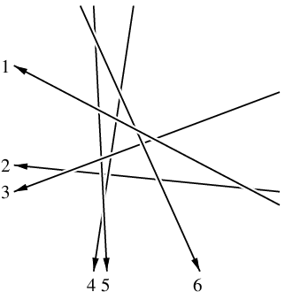
Figure 2 shows a labeled and oriented configuration of six skew lines with linking matrix

Two symmetric matrices $X$ and $Y$ are switching-equivalent if

where $P$ is a permutation matrix and $D$ is a diagonal matrix with $d_{i,i}\in\{\pm 1\}$. Since $P$ and $D$ are orthogonal, we have $(PD)^{-1}=D^{t}P^{t}=DP^{t}$. Switching-equivalent matrices are thus conjugate and have the same characteristic polynomial.

The set of vorticities (also called homological equivalence class or chiral signature), introduced by Viro [12], is a classical and well-known invariant for configurations of skew lines. We sketch below briefly the well-known proof that it corresponds to the switching class of an associated linking matrix.

We prefer to work with switching classes corresponding to symmetric matrices (up to conjugation by signed permutation matrices) with zero diagonal and off-diagonal coefficients in $\{\pm 1\}$.

The vorticity $\hbox{vort}(L_{i},L_{j},L_{k})$ of three lines (see [12, Section 2] or [4, Section 3]) is defined as the product $x_{i,j}x_{j,k}x_{k,i}\in\{\pm 1\}$ of the signs for the corresponding three crossings. The result is independent of the chosen orientations for $L_{i},L_{j},L_{k}$, classifies the skew-configuration $\{L_{i},L_{j},L_{k}\}$ up to isotopy and yields an invariant

Let us remark that almost all authors use the terminology linking coefficient instead of vorticity. This is slightly confusing since the linking coefficient denotes also the isotopy type of a pair of oriented skew lines.

The set of vorticities is the list of vorticities $\hbox{vort}(L_{i},L_{j},L_{k})$ for all triplets of lines $\{L_{i},L_{j},L_{k}\}$ in a configuration of skew lines.

Sets of vorticities (defining a two-graph, see [14]) and switching classes are equivalent. Indeed, vorticities of a configuration of skew lines $\mathcal{C}$ can easily be retrieved from a linking matrix for $\mathcal{C}$. Conversely, given all vorticites ${\rm vort}(L_{i},L_{j},L_{k})$ of a configuration $\mathcal{C}=\{L_{1},\dots,L_{n}\}$, choose an orientation of the first line $L_{1}$. Orient the remaining lines $L_{2},\dots,L_{n}$ such that they cross $L_{1}$ positively. A linking matrix $X$ for $\mathcal{C}$ is given by $x_{1,i}=x_{i,1}=1$ for $i$ such that $2\leq i\leq n$ and $x_{a,b}={\rm vort}(L_{1},L_{a},L_{b})$ for $2\leq a\not=b\leq n$.

Two configurations of skew lines are homologically equivalent (the terminology refers to properties of the complement, endowed with a suitable extra-structure, of a configuration in $\mathbb{RP}^{3}$) if there exists a bijection between their lines, which preserves all vorticities. Two configurations are homologically equivalent if and only if they have switching-equivalent linking matrices.

The sign indeterminacy in linking matrices representing switching classes makes their use more difficult. A satisfactory answer addressing this problem will be given in Section 4.1 for switching classes of odd order. For even orders, there seems to be no completely satisfactory way to get rid of all sign-indeterminacies, see Section 4.2.

In this section we study invariants of computational cost $O(n^{2})$ for switching classes of order $n$.

The behaviour of switching classes depends on the parity of their order.

Switching classes of odd order $2n-1$ are in bijection with Eulerian graphs. This endows the lines of a skew configuration consisting of an odd number of lines with a semi-orientation (a canonical orientation, up to global change) which we call the Eulerian semi-orientation. An Eulerian semi-orientation induces a partition of the lines into equivalence classes by counting their number of positive crossings. We consider the case of odd order in Section 4.1.

The situation for switching classes of even order $2n$ is more complicated. We replace Eulerian graphs appearing for odd orders by a suitable kind of rooted binary trees which we call Euler trees. The leaves of the Euler tree induce again a natural partition, called the Euler partition, of the set of lines into equivalence classes of even cardinalities. Section 4.2 deals with the even case.

A construction of Mazurovskiĭ originally called the isotopy join (or spindle) associates a configuration of $n$ skew lines to every permutation of $n$ letters. We recall that a spindle is a configuration of skew lines with all lines intersecting an oriented auxiliary line $A$, called its axis. A spindle-configuration (or a spindle structure) is a configuration of skew lines isotopic to a spindle.

The orientation of the axis $A$ induces a linear order $L_{1}<\dots<L_{n}$ on the $n$ lines of a spindle $C$. Each line $L_{i}\in C$ defines a plane $\Pi_{i}$ containing $L_{i}$ and the axis $A$.

A second oriented auxiliary line $B$ (called a directrix) in general position with respect to $A,\Pi_{1},\dots,\Pi_{n}$ and crossing $A$ negatively, intersects the planes $\Pi_{1},\dots,\Pi_{n}$ at points $\sigma(L_{i})=B\cap\Pi_{i}$. One can assume $\sigma(L_{i})\in L_{i}$ by a suitable rotation fixing $A\cap\Pi_{i}$ of the plane $\Pi_{i}$ containing $L_{i}$. Since the orientation of $B$ induces a linear order on the points $\sigma(L_{i})$, we get a spindle-permutation (still denoted) $i\longmapsto\sigma(i)$ of the set $\{1,\dots,n\}$ by identifying the two linearly ordered sets $L_{1},\dots,L_{n}$ and $\sigma(L_{1}),\dots,\sigma(L_{n})$ in the obvious way with $\{1,\dots,n\}$. Figure 6 displays an example corresponding to $\sigma(1)=1,\ \sigma(2)=4,\ \sigma(3)=2,\ \sigma(4)=5,\ \sigma(5)=3$.

A linking matrix $X$ of a spindle $C$ is easily computed as follows. Transform $C$ isotopically into a spindle with oriented axis $A$ and directrix $B$ as above. Orient a line $L_{i}$ from $L_{i}\cap A$ to $\sigma(L_{i})=L_{i}\cap B$. A straightforward computation shows that the linking matrix $X$ of this labeled and oriented configuration of skew lines has coefficients

where $\hbox{sign}(0)=0$ and $\hbox{sign}(x)=\frac{x}{|x|}$ for $x\not=0$ and where $\sigma$ is the corresponding spindle-permutation.

The linking matrix of Figure 6 is

Two spindle-permutations are equivalent (see [4, Section 15]), and give rise to isotopic spindle configurations, if they are equivalent under the equivalence relation generated by

1. (1)

   (Circular move)

   $$\sigma\sim\mu\hbox{ if }\mu(i)=(s+\sigma((i+t)\pmod{n}))\pmod{n}$$

   for some integers $0\leq s,t<n$ (all integers are modulo $n$).

2. (2)

   (Vertical reflection of a block or local reversal) $\sigma\sim\mu$ if $\sigma([1,k])=[1,k]$ and

   $$\mu(i)=\left\{\begin{array}[]{ll}k+1-\sigma(k+1-i)&i\leq k\cr\sigma(i)&i>k\end{array}\right.$$

   for some integer $k\leq n$ (see Figure 7).

   

3. (3)

   (Horizontal reflection of a block or local inversion) $\sigma\sim\mu$ if there exists an integer $1<k\leq n$ such that $\sigma([1,k])=[1,k]$ and

   $$\mu(i)=\left\{\begin{array}[]{ll}\sigma^{-1}(i)&i\leq k\cr\sigma(i)&i>k\end{array}\right.$$

   (see Figure 8).

   

Permutations giving rise to linking matrices in a common switching class are spindle-equivalent by Corollary 1.2.

Given a switching class represented by a matrix $X$, the following algorithm constructs a spindle-permutation (which is unique up to spindle-equivalence) with linking matrix in the switching class of $X$ or proves non-existence of such a permutation.

The second author wishes to thank the Institut Fourier where most of this work was done and Mikhail Zaidenberg for hosting his stay.

References

- [1] R. Bacher and D. Garber, Spindle configurations of skew lines, Geom. Topo. 11 (2007), 1049–1081.
- [2] A. Borobia and V. F. Mazurovskiĭ, On diagrams of configurations of skew lines of , Amer. Math. Soc. Transl. (2) 173 (1996), 33–40.
- [3] A. Borobia and V. F. Mazurovskiĭ, Nonsingular configurations of lines in , J. Knot Theory & Ramif. 6(6) (1997), 751–783.
- [4] H. Crapo and R. Penne, Chirality and the isotopy classification of skew lines in projective 3-space, Adv. Math. 103 (1994), 1–106.
- [5] Y. V. Drobotukhina, An analogue of the Jones polynomials for links in and a generalization of the Kauffman-Murasugi theorem, Leningrad Math. J. 2(3) (1991), 613–630.
- [6] S. I. Khashin, Projective graph theory and configurations of lines, J. Math. Sci. (New-York) 91(6) (1998), 3532–3541.
- [7] S. I. Khashin and V. F. Mazurovskiĭ, Stable equivalence of real projective configurations, Amer. Math. Soc. Transl. (2) 173 (1996), 119–140.
- [8] V. F. Mazurovskiĭ, Configurations of at most six lines in , Real Algebraic Geometry, Proceedings of the conference held in Rennes, France, June 24–28, 1991, Lecture Notes in Math. 1524 (1992), 354–371.
- [9] V. F. Mazurovskiĭ, Configurations of six skew lines (Russian. English summary) Zap. Nauchn. Sem. Leningrad. Otdel. Mat. Inst. Steklov. (LOMI) 167 (1988), Issled. Topol. 6, 121–134, 191; translation in: J. Soviet Math. 52(1) (1990), 2825–2832.
- [10] J. J. Seidel, Graphs and two-graphs, Proc. 5th Southeastern Conf. on Combinatorics, Graph Theory and Computing, Utilitas Mathematica Publishing Inc., Winnipeg, Canada, 1974.
- [11] N. J. A. Sloane (editor), The On-Line Encyclopedia of Integer Sequences, http://www.research.att.com/˜njas/sequences/.
- [12] O. Y. Viro, Topological problems concerning lines and points of three-dimensional space, Soviet Math. Dokl. 2(32) (1985), 528–531.
- [13] O. Y. Viro and Y. V. Drobotukhina, Configurations of skew lines, Leningrad Math. J. 1(4) (1990), 1027–1050, or (updated version): http://www.math.uu.se/˜oleg/skewlines/index.html, arXiv: math.GT/0611374.
- [14] T. Zaslavsky, Glossary of Signed and Gain Graphs and Allied Areas, The Electronic Journal of Combinatorics (1998), Dynamic Surveys in Combinatorics DS9, 41 pages.