Probing surface states of topological insulator: Kondo effect and Friedel oscillation under magnetic field

Minh-Tien Tran^1,2 and Ki-Seok Kim^1,3 Affiliation: ¹Asia Pacific Center for Theoretical Physics, Pohang, Gyeongbuk 790-784, Republic of Korea
²Institute of Physics, Vietnamese Academy of Science and Technology, P.O.Box 429, 10000 Hanoi, Vietnam
³Department of Physics, Pohang University of Science and Technology, Pohang, Gyeongbuk 790-784, Korea

Abstract

We address three issues on the role of magnetic impurities in the surface state of a three dimensional topological insulator. First, we prove that the Kondo effect of the topological surface is essentially the same as that of the graphene surface, demonstrating that an effective impurity action of the topological surface coincides with that of the graphene surface. Second, we study the role of the $z$ -directional magnetic field ( $h$ ) in the Kondo effect, and show that the peak splitting in the impurity local density of states does not follow the $h$ -linear behavior, the typical physics in the soft-gap Kondo model. We discuss that the origin is spin locking in the helical surface. Third, we examine the Friedel oscillation around the magnetic impurity. It turns out that the pattern of Friedel oscillation in the helical surface is identical to that of the graphene surface, displaying the inverse-square behavior $\sim r^{-2}$ if the inter-valley scattering is not introduced in the graphene case. However, introduction of the magnetic field leads the electron density of states from the inverse-square physics to the inverse behavior $\sim r^{-1}$ in the topological insulator’s surface while it still remains as $\sim r^{-2}$ in the graphene Kondo effect. We discuss that this originates from spin flipping induced by magnetic field.

pacs

71.27.+a, 75.20.Hr, 73.90.+f, 75.30.Mb

I Introduction

It has been one of the main research interests to understand topological states of matter in modern condensed matter physics.[1] Electrons in two dimensions under strong magnetic field form such a topological state, exhibiting the quantum Hall effect (QHE) with gapless chiral edge modes protected by topology.[2] Later, Haldane proposed an interesting toy model to show the QHE without Landau levels, basically the tight-binding model for spinless electrons in the honeycomb lattice with a complex next-nearest-neighbor hopping parameter.[3] Recently, Kane and Mele extended the Haldane model into the case of spinful electrons, where each spin observes an opposite fictitious magnetic flux, realized by the spin-orbit coupling and preserving time reversal symmetry.[4] Analogous with the QHE, this insulating state shows the spin QHE, where the difference of the spin $\uparrow$ and $\downarrow$ Hall conductances is quantized. When the spin quantum number is not conserved due to the presence of the Rashba-type spin-orbit interaction, the spin Hall conductance cannot be used for topological characterization. Kane and Mele proposed the Z₂ index, counting the number of helical edge states with modular $2$ , and concluded that the odd Z₂ index state corresponds to a topological state of an insulator, which cannot be adiabatically connected to the even Z₂ state of a trivial insulator.[4]

Immediately, it was performed three dimensional generalization of the two dimensional Z₂ topological insulator.[5, 6, 7] It turns out that the surface state of the three dimensional topological insulator has an odd number of helical Dirac fermions,[8] identified with an odd Z₂ index, where spins are locked along the momentum direction on the surface. Since there is no QHE analogue in three dimensions, the three dimensional topological insulator has been regarded as a new quantum state of matter.

An interesting prediction is associated with the stability of the helical metallic state against time reversal symmetric perturbation, where it should be stable against Anderson localization independent of the disorder strength.[9] In addition, the topological $\theta$ term appears due to the chiral anomaly in the field theory context, giving rise to electric polarization along the magnetic field direction when time reversal symmetry breaking field is applied infinitesimally.[10, 11]

Although the topological insulator was now verified experimentally,[12, 13, 14, 15] the angle reserved photo emission spectroscopy (ARPES) is the only experimental probe, not performed on the table top. In this respect it is desirable to propose table top experiments for three dimensional topological insulators. Recently, an experimental realization of the magnetic doping on the surface of three-dimensional topological insulator was reported.[16]

In this paper we propose how to probe the surface state of the topological insulator, investigating the Kondo effect and Friedel oscillation under magnetic field. Since spins of host electrons are locked along the momentum in the topological surface, one may expect under-screening for a magnetic impurity in contrast with the soft-gap Kondo physics [17] expected to arise in the graphene surface.[18] However, it turns out that the Kondo effect of the topological surface is essentially the same as that of the graphene surface. Integrating over host electrons, we also prove that an effective impurity action of the helical metal coincides with that of the soft-gap Anderson model. This precise demonstration tells us exact impurity screening at hybridization enough to overcome the vanishing density of states. In order to distinguish the Kondo effect of the topological surface from the soft-gap Kondo effect, we introduce magnetic field in the $z$ -direction ( $h$ ). We show that the peak splitting in the impurity local density of states does not follow the $h$ -linear behavior, the typical physics in the soft-gap Anderson or Kondo model. We derive an analytic expression based on the picture of spin locking in the helical surface.

Finally, we examine the feedback effect of the impurity dynamics to host electrons, evaluating the host-electron local density of states (LDOS) and revealing the Friedel oscillation around the magnetic impurity. The LDOS is measurable by Fourier transformation scanning tunneling spectroscopy (FTSTS). The FTSTS measurements have been developed for graphene,[19, 20] as well as other two dimensional materials.[21, 22] The LDOS in graphene was also investigated theoretically.[23] It turns out that the pattern of Friedel oscillation in the topological surface is identical to that of the graphene surface without magnetic field, displaying the inverse-square behavior $\sim r^{-2}$ if the inter-valley scattering is not introduced in the graphene case, where $r$ is the distance from the impurity position. However, introduction of the magnetic field leads the LDOS from the inverse-square physics to the inverse behavior $\sim r^{-1}$ in the topological insulator’s surface while it still remains as $\sim r^{-2}$ in the graphene Kondo effect. We discuss that this originates from spin flipping induced by magnetic field.

This study addresses three issues on the role of magnetic impurities in the surface state of a three dimensional topological insulator. First, we prove that the Kondo effect of the topological surface is essentially the same as that of the graphene surface. Second, we study the role of the $z$ -directional magnetic field ( $h$ ) in the Kondo effect, which turns out to differ from the typical physics in the soft-gap Kondo model. Third, we examine the effect of the magnetic field on the Friedel oscillation around the magnetic impurity. The previous studies of Refs. 24 and 25 addressed the first issue, where the effect of the magnetic field is absent. The Ref. 24 uses the variational method to study the Kondo effect, which is an approximation, thus not a rigorous proof for the equivalence of the Kondo effect in the topological insulator and graphene, although this study can give fruitful information such as spin correlations. The Ref. 25 also pointed out the equivalence based on a different choice of the unitary transformation, and we compare these two different transformations. However, the other two issues have been discussed only in our study, and they are essential to probe the surface states of topological insulators.

The present paper is organized as follows. In Sec. II we derive an effective impurity action from the Anderson model, mapping the model into an effective one dimensional action and integrating over such one dimensional host electrons. Performing the slave-boson mean-field analysis, we show that the peak splitting of the impurity density of states under magnetic field differs from the standard Zeeman energy proportional to the magnetic field. In section III we present the host-electron LDOS and its local charge density. They reveal that the decay of the Friedel oscillation changes from an inverse-square law to an inverse law, applying magnetic field. In section IV summary and discussion are presented.

II Impurity dynamics

II.1 Equivalence between the Kondo effect of the helical metal and the soft-gap Anderson model

II.1.1 An effective impurity action in the helical metal

We start from an Anderson model in two dimensions

	$\displaystyle H_{\text{hel}}$	$\displaystyle=$	$\displaystyle\sum\limits_{\mathbf{k}\sigma\sigma^{\prime}}c_{\mathbf{k}\sigma}^{\dagger}[v_{F}(\mathbf{k}\cdot{\boldsymbol{\sigma}})_{\sigma\sigma^{\prime}}-\mu_{\sigma}\delta_{\sigma\sigma^{\prime}}]c_{\mathbf{k}\sigma^{\prime}}+{\displaystyle\sum\limits_{\sigma}}E_{f\sigma}f_{\sigma}^{\dagger}f_{\sigma}$		(1)
		$\displaystyle+$	$\displaystyle{\displaystyle\sum\limits_{\mathbf{k}\sigma}}V\left(\mathbf{k}\right)f_{\sigma}^{\dagger}c_{\mathbf{k}\sigma}+\text{H.c.}+Un_{\uparrow}^{f}n_{\downarrow}^{f}.$		(1)

$c_{\mathbf{k}\sigma}^{\dagger}$ ( $c_{\mathbf{k}\sigma}$ ) is the creation (annihilation) operator for host electrons with momentum $\mathbf{k}=(k_{x},k_{y})$ . This metallic host is given by the surface of the topological insulator, where the $\mathbf{k}\cdot{\boldsymbol{\sigma}}$ term locks the electron spin to its momentum, named as helical metal. $v_{\text{F}}$ is the Fermi velocity, and $\sigma^{x}$ , $\sigma^{y}$ are the Pauli matrices. $\sigma=\pm 1$ is the spin index, and $\mu_{\sigma}=\mu+\sigma h$ is an effective chemical potential, where $h$ is the magnetic field. $f_{\sigma}^{\dagger}$ ( $f_{\sigma}$ ) represents the creation (annihilation) operator for the magnetic impurity. $E_{f\sigma}=E_{f}-\sigma h$ is an effective impurity energy level with the Zeeman energy contribution. $U$ is the Coulomb interaction at the impurity site. $V(\mathbf{k})$ is the hybridization between the impurity and helical electrons, assumed to be $V(\mathbf{k})=V$ for simplicity.

In order to map this Hamiltonian to one dimensional model, we write $\mathbf{k}=k(\cos(\phi),\sin(\phi))$ , where $k=|\mathbf{k}|$ and $\phi$ is the angle of the momentum $\mathbf{k}$ from the $x$ -axis. The Hamiltonian for helical electrons without magnetic field can be rewritten as

H^{\text{c}}_{\text{hel}}=\sum\limits_{\mathbf{k}\sigma\sigma^{\prime}}\varepsilon_{k}c_{\mathbf{k}\sigma}^{\dagger}M_{\sigma\sigma^{\prime}}(\phi)c_{\mathbf{k}\sigma^{\prime}},

(2)

where $\varepsilon_{k}=v_{\text{F}}k$ is the energy dispersion, and

\displaystyle\hat{M}\left(\phi\right)=\left(\begin{array}[c]{cc}0&e^{-i\phi}\\ e^{i\phi}&0\end{array}\right)

expresses the spin-momentum coupling. Introducing the unitary transformation

\displaystyle\hat{U}(\phi)=\frac{1}{\sqrt{2}}\left(\begin{array}[c]{cc}1&1\\ e^{i\phi}&-e^{i\phi}\end{array}\right),

the Hamiltonian (2) is diagonalized as follows

H^{\text{c}}_{\text{hel}}=\sum\limits_{\mathbf{k}\sigma}\varepsilon_{k}\sigma\gamma_{\mathbf{k}\sigma}^{\dagger}\gamma_{\mathbf{k}\sigma},

(9)

where $\hat{\gamma}_{\mathbf{k}}=\hat{U}^{\dagger}(\phi)\hat{c}_{\mathbf{k}}$ . Expanding the $\gamma_{\mathbf{k}\sigma}$ operator in the basis of angular-momentum eigenmodes [17]

\displaystyle\gamma_{\mathbf{k}\sigma}=\frac{1}{\sqrt{k}}\frac{1}{\sqrt{2\pi}}\sum\limits_{m}e^{im\phi}\gamma_{m\sigma}(k),

(10)

where $m$ is an integer representing angular momentum, we rewrite the Hamiltonian (9) as

\displaystyle H^{\text{c}}_{\text{hel}}=\sum\limits_{m\sigma}\int\limits_{0}^{\infty}dk\varepsilon_{k}\sigma\gamma_{m\sigma}^{\dagger}(k)\gamma_{m\sigma}(k).

(11)

The hybridization term in Hamiltonian (1) becomes

	$\displaystyle H^{\text{hyb}}_{\text{hel}}$	$\displaystyle=$	$\displaystyle\frac{\sqrt{N}V}{2\sqrt{\pi}}\int\limits_{0}^{\infty}dk\sqrt{k}[f_{\uparrow}^{\dagger}\gamma_{0\uparrow}(k)+f_{\uparrow}^{\dagger}\gamma_{0\downarrow}(k)$		(12)
		$\displaystyle+$	$\displaystyle f_{\downarrow}^{\dagger}\gamma_{-1\uparrow}(k)-f_{\downarrow}^{\dagger}\gamma_{-1\downarrow}(k)]+\text{H.c.}$		(12)

in the $\gamma_{m\sigma}$ basis, where $N$ is the number of surface states. Note that only the $s$ - ( $m=0$ ) and $p$ - ( $m=-1$ ) wave components contribute to the hybridization between the impurity and conduction electrons. This is typical in the Dirac spectrum,[17] resulting from ( $1$ , $e^{i\phi}$ ) in the unitary matrix while only the $s$ -wave scattering is relevant in the presence of the Fermi surface.

The Zeeman term is

\displaystyle H^{h}_{\text{hel}}=-h\sum\limits_{m}\int\limits_{0}^{\infty}dk[\gamma_{m\uparrow}^{\dagger}(k)\gamma_{m\downarrow}(k)+\gamma_{m\downarrow}^{\dagger}(k)\gamma_{m\uparrow}(k)]

(13)

for helical electrons. Remember that the magnetic field is applied in the $z$ -direction. Since spins are locked along the momentum direction in the plane, the magnetic field should flip the spin in order to get its $z$ -component. As a result, helical electrons at the momentum $k_{F}$ couple to those at $-k_{F}$ in the presence of magnetic field. As will be discussed in the next section, this is the reason why the inverse square behavior in the Friedel oscillation pattern turns into the inverse form. On the other hand, this spin-flip process is not introduced into the conventional soft-gap Anderson model by the magnetic field, showing the inverse square law as long as the inter-valley scattering is not taken into account.[23]

It is convenient to consider

$\displaystyle\psi_{k\uparrow}$	$\displaystyle=$	$\displaystyle\frac{1}{\sqrt{2}}(\gamma_{0\uparrow}(k)+\gamma_{0\downarrow}(k)),$	(14)
$\displaystyle\psi_{k\downarrow}$	$\displaystyle=$	$\displaystyle\frac{1}{\sqrt{2}}(\gamma_{-1\uparrow}(k)-\gamma_{-1\downarrow}(k)),$	(15)
$\displaystyle\varphi_{k\uparrow}$	$\displaystyle=$	$\displaystyle\frac{1}{\sqrt{2}}(\gamma_{0\uparrow}(k)-\gamma_{0\downarrow}(k)),$	(16)
$\displaystyle\varphi_{k\downarrow}$	$\displaystyle=$	$\displaystyle\frac{1}{\sqrt{2}}(\gamma_{-1\uparrow}(k)+\gamma_{-1\downarrow}(k)).$	(17)

One can verify that these operators satisfy the fermionic anticommutation relations. Rewriting the Hamiltonian (1) in this new basis, we obtain

$\displaystyle H_{\text{hel}}$	$\displaystyle=$	$\displaystyle\sum\limits_{\sigma}\int\limits_{0}^{\infty}dk\varepsilon_{k}(\psi_{k\sigma}^{\dagger}\varphi_{k\sigma}+\varphi_{k\sigma}^{\dagger}\psi_{k\sigma})$	(18)
	$\displaystyle-$	$\displaystyle\sum\limits_{\sigma}\int\limits_{0}^{\infty}dk(\mu_{\sigma}\psi_{k\sigma}^{\dagger}\psi_{k\sigma}+\mu_{-\sigma}\varphi_{k\sigma}^{\dagger}\varphi_{k\sigma})$
	$\displaystyle+$	$\displaystyle\sum\limits_{\sigma}E_{f\sigma}f_{\sigma}^{\dagger}f_{\sigma}+Un_{\uparrow}^{f}n_{\downarrow}^{f}$
	$\displaystyle+$	$\displaystyle\sum\limits_{\sigma}\frac{\sqrt{N}V}{\sqrt{2\pi}}\int\limits_{0}^{\infty}dk\sqrt{k}f_{\sigma}^{\dagger}\psi_{k\sigma}+\text{H.c.},$

where the impurity couples to only $\psi_{\sigma}$ -electrons.

Integrating over the $\varphi_{\sigma}$ fields, we obtain the effective action

	$\displaystyle S_{\text{hel}}=\!\!\sum\limits_{\sigma}\!\!\int\limits_{0}^{\beta}\!\!d\tau\!\!\int\limits_{0}^{\beta}\!\!d\tau^{\prime}\!\!\!\!\int\limits_{0}^{\infty}\!\!dk\psi_{k\sigma}^{\dagger}(\tau)[g_{c\sigma}^{\text{hel}}(k,\tau-\tau^{\prime})]^{-1}\psi_{k\sigma}(\tau^{\prime})$
	$\displaystyle+\sum\limits_{\sigma}\int\limits_{0}^{\beta}d\tau f_{\sigma}^{\dagger}(\tau)[\partial_{\tau}+E_{f\sigma}]f_{\sigma}(\tau)+U\int\limits_{0}^{\beta}d\tau n_{\uparrow}^{f}(\tau)n_{\downarrow}^{f}(\tau)$
	$\displaystyle+\sum\limits_{\sigma}\frac{\sqrt{N}V}{\sqrt{2\pi}}\int\limits_{0}^{\beta}d\tau\int\limits_{0}^{\infty}dk\sqrt{k}f_{\sigma}^{\dagger}(\tau)\psi_{k\sigma}(\tau)+\text{H.c.},\;\;\;\;\;\;\;$		(19)

where

\displaystyle g_{c\sigma}^{\text{hel}}(k,i\omega)=\frac{i\omega+\mu_{-\sigma}}{(i\omega+\mu_{\sigma})(i\omega+\mu_{-\sigma})-(\varepsilon_{k})^{2}}

(20)

is the $\psi_{\sigma}$ Green’s function. Integration of the $\psi_{\sigma}$ fields gives rise to an effective action for dynamics of the magnetic impurity on the surface of the topological insulator

	$\displaystyle S_{\text{hel}}$	$\displaystyle=$	$\displaystyle\sum\limits_{\sigma}\int\limits_{0}^{\beta}d\tau f_{\sigma}^{\dagger}(\tau)[\delta(\tau-\tau^{\prime})(\partial_{\tau}+E_{f\sigma})$		(21)
		$\displaystyle+$	$\displaystyle\Delta_{\sigma}^{\text{hel}}(\tau-\tau^{\prime})]f_{\sigma}(\tau^{\prime})+U\int\limits_{0}^{\beta}d\tau n_{\uparrow}^{f}(\tau)n_{\downarrow}^{f}(\tau),\;\;\;$		(21)

where

\displaystyle\Delta_{\sigma}^{\text{hel}}(i\omega)=\frac{N|V|^{2}}{2\pi}\int\limits_{0}^{\infty}dkkg_{c\sigma}^{\text{hel}}(k,i\omega)

(22)

is the hybridization function. Using the Lorentzian cutoff,[17] we obtain the hybridization function

	$\displaystyle\Delta_{\sigma}^{\text{hel}}(i\omega)=\frac{N\|V\|^{2}}{2\pi}\int\limits_{0}^{\infty}dkkg_{c\sigma}^{\text{hel}}(k,i\omega)\frac{2}{\pi}\frac{\Lambda v_{F}}{v_{F}^{2}k^{2}+\Lambda^{2}}$
	$\displaystyle=-\Gamma\frac{2\Lambda(i\omega+\mu-\sigma h)}{(i\omega+\mu)^{2}-h^{2}+\Lambda^{2}}\log\frac{\Lambda^{2}}{h^{2}-(i\omega+\mu)^{2}},$		(23)

where $\Lambda$ is a cutoff in energy and $\Gamma=N|V|^{2}/4\pi^{2}v_{F}$ .

II.1.2 An effective impurity action in the soft gap metal

We consider the soft-gap Anderson model

$\displaystyle H_{\text{sg}}$	$\displaystyle=$	$\displaystyle\sum\limits_{\mathbf{k}\alpha\alpha^{\prime}\sigma}c_{\mathbf{k}\alpha\sigma}^{\dagger}[v_{F}(\mathbf{k}\cdot{\boldsymbol{\sigma}})_{\alpha\alpha^{\prime}}-\mu_{\sigma}\delta_{\alpha\alpha^{\prime}}]c_{\mathbf{k}\alpha^{\prime}\sigma}$	(24)
	$\displaystyle+$	$\displaystyle{\displaystyle\sum\limits_{\sigma}}E_{f\sigma}f_{\sigma}^{\dagger}f_{\sigma}+Un_{\uparrow}^{f}n_{\downarrow}^{f}$
	$\displaystyle+$	$\displaystyle{\displaystyle\sum\limits_{\mathbf{k}\alpha\sigma}}V\left(\mathbf{k}\right)f_{\sigma}^{\dagger}c_{\mathbf{k}\alpha\sigma}+\text{H.c.}.$

The notation in the Hamiltonian (24) is the same as that in Eq. (1) except for the conduction electrons which now have an additional branch notation $\alpha,\alpha^{\prime}=\pm 1$ , associated with the Pauli matrix $\boldsymbol{\sigma}_{\alpha\alpha^{\prime}}$ . This may be interpreted as pseudospin, which can result from two sublattices in graphene. [18] In addition to this pseudospin index, there exists another Dirac cone in graphene, called valley. In this study we take into account only one valley to focus on the comparison with the helical metal. In the soft-gap metal momentum is not tied to the electron spin, instead the pseudospin. This feature differs from helical electrons.

Proceeding in the same way as in the previous subsection, we obtain

$\displaystyle H_{\text{sg}}$	$\displaystyle=$	$\displaystyle\sum\limits_{m=0,-1}\sum\limits_{\alpha\sigma}\int\limits_{0}^{\infty}dkk(\alpha\varepsilon_{k}+\mu_{\sigma})\gamma_{m\alpha\sigma}^{\dagger}(k)\gamma_{m\alpha\sigma}(k)$	(25)
	$\displaystyle+$	$\displaystyle\sum\limits_{\sigma}E_{f\sigma}f_{\sigma}^{\dagger}f_{\sigma}+Un_{\uparrow}^{f}n_{\downarrow}^{f}$
	$\displaystyle+$	$\displaystyle\frac{\sqrt{N}V}{2\sqrt{\pi}}\sum\limits_{\sigma}\int\limits_{0}^{\infty}dk\sqrt{k}f_{\sigma}^{\dagger}[\gamma_{0,+,\sigma}(k)+\gamma_{0,-,\sigma}(k)$
	$\displaystyle+$	$\displaystyle\gamma_{-1,+,\sigma}(k)-\gamma_{-1,-,\sigma}(k)]+\text{H.c.},$

where the $\gamma_{m\alpha\sigma}(k)$ basis diagonalizes the conduction electron part of Hamiltonian (24). Note that the pseudospin $\alpha$ plays the same role as the spin of the helical metal, where the pseudospin mixing appears in the hybridization term.

We introduce $\psi_{1,\sigma}(k)=\gamma_{0,+,\sigma}(k)$ for $k\geq 0$ , and $\psi_{1,\sigma}(k)=\gamma_{0,-,\sigma}(k)$ for $k<0$ ; $\psi_{2,\sigma}(k)=\gamma_{-1,+,\sigma}(k)$ for $k\geq 0$ , and $\psi_{2,\sigma}(k)=-\gamma_{-1,-,\sigma}(k)$ for $k<0$ . These new operators allow us to rewrite the Hamiltonian (25) in the following way

$\displaystyle H_{\text{sg}}$	$\displaystyle=$	$\displaystyle\sum\limits_{\alpha=1,2;\sigma}\int\limits_{-\infty}^{\infty}dk(\varepsilon_{k}-\mu_{\sigma})\psi_{\alpha\sigma}^{\dagger}(k)\psi_{\alpha\sigma}(k)$	(26)
	$\displaystyle+$	$\displaystyle\sum\limits_{\sigma}E_{f\sigma}f_{\sigma}^{\dagger}f_{\sigma}+Un_{\uparrow}^{f}n_{\downarrow}^{f}$
	$\displaystyle+$	$\displaystyle\frac{\sqrt{N}V}{2\sqrt{\pi}}\sum\limits_{\alpha=1,2;\sigma}\int\limits_{-\infty}^{\infty}dk\sqrt{\|k\|}f_{\sigma}^{\dagger}\psi_{\alpha\sigma}(k)+\text{H.c.}\;\;\;$

Note that the magnetic field in the soft-gap metal couples to electrons with the same spin and pseudospin. There is no spin-flip or pseudospin-flip process, induced by magnetic field.

Integrating over the $\psi_{\alpha\sigma}$ field, we obtain an effective impurity action from the soft-gap Anderson model

	$\displaystyle S_{\text{sg}}$	$\displaystyle=$	$\displaystyle\sum\limits_{\sigma}\int\limits_{0}^{\beta}d\tau f_{\sigma}^{\dagger}(\tau)[\delta(\tau-\tau^{\prime})(\partial_{\tau}+E_{f\sigma})$		(27)
		$\displaystyle+$	$\displaystyle\Delta_{\sigma}^{\text{sg}}(\tau-\tau^{\prime})]f_{\sigma}(\tau^{\prime})+U\int\limits_{0}^{\beta}d\tau n_{\uparrow}^{f}(\tau)n_{\downarrow}^{f}(\tau),\;\;\;$		(27)

where

	$\displaystyle\Delta_{\sigma}^{\text{sg}}(i\omega)$	$\displaystyle=$	$\displaystyle\frac{N\|V\|^{2}}{2\pi}\sum\limits_{\alpha}\int\limits_{-\infty}^{\infty}dk\|k\|\frac{1}{i\omega+\mu_{\sigma}-\varepsilon_{k}}$		(28)
		$\displaystyle=$	$\displaystyle-\Gamma\frac{4\Lambda(i\omega+\mu_{\sigma})}{(i\omega+\mu_{\sigma})^{2}+\Lambda^{2}}\log\frac{-\Lambda^{2}}{(i\omega+\mu_{\sigma})^{2}}\;\;\;$		(28)

is the hybridization function.

II.1.3 Discussion

It is quite interesting to see that the effective impurity action in the helical metal is essentially identical with that in the graphene case without magnetic field. The only difference is the factor $2$ in the hybridization function of the soft-gap metal, resulting from the pseudospin symmetry. This completes our proof that the magnetic impurity on the surface of the topological insulator is screened exactly, the same as the Kondo effect in the soft-gap Anderson model.[17] The identity of the effective impurity action in the helical metal and graphene was also pointed out in Ref. 25.

An interesting point is the choice of the unitary matrix for diagonalization. In this paper we choose the single-valued function as the unitary matrix, given by $e^{i\phi}$ . On the other hand, the previous studies [24, 25] took the double-valued function $e^{i\phi/2}$ in the unitary matrix. Although this kind of non-single-valued function can be utilized in principle, the branch-cut should be taken into account with an additional phase factor carefully. However, an effective impurity action based on this double-valued unitary transformation is completely identical with that based on the single-valued unitary transformation. In appendix we perform the same procedure to find the effective impurity action.

II.2 U(1) slave-boson mean-field analysis in the presence of magnetic field

Although the Kondo effect in the helical metal is completely the same as that of the soft-gap Anderson model without magnetic field, it becomes much different, applying magnetic field. This originates from the fact that the magnetic field gives rise to the spin-flip process in the helical metal while there is no such a term in the graphene. This is reflected on the magnetic-field dependence of the hybridization function. To reveal the effect of the magnetic field, we use the slave-boson mean-field approximation in the $U\rightarrow\infty$ limit. The electron operator at the impurity site is decomposed as $f_{\sigma}=d_{\sigma}\hat{b}^{\dagger}$ , where $d_{\sigma}$ is a fermion operator and $b$ is a boson one.[26] A constraint should be imposed to match the Hilbert space of the original electron representation with that of the slave-boson expression, given by

\displaystyle\hat{b}^{\dagger}\hat{b}+\sum_{\sigma}d_{\sigma}^{\dagger}d_{\sigma}=1.

(29)

In the mean-field approximation the boson operator is replaced by its average value $\langle\hat{b}\rangle=b$ , and the constraint equation (29) is taken into account by its average version. The impurity Green’s function is given by

\displaystyle G_{d\sigma}(\omega)=\frac{1}{\omega-\tilde{E}_{f\sigma}-b^{2}\Delta_{\sigma}(\omega)},

(30)

where $\tilde{E}_{f\sigma}=E_{f\sigma}+\lambda$ is an effective energy level and $\lambda$ is the Lagrange multiplier to impose the slave-boson constraint. We consider the chemical potential of conduction electrons slightly above the Dirac point, i.e., $\mu>0$ . Fig. 1 shows the splitting energy of the spin $\uparrow$ and $\downarrow$ Kondo peaks in the spectral density of the impurity under magnetic field. In the case of the soft-gap Anderson model $D=2h$ results, as expected. On the other hand, the Kondo-peak splitting in the helical metal deviates from the typical $h$ -linear behavior. This property distinguishes the Kondo effect of the helical metal from that of the soft-gap Anderson model and would be observed experimentally.

Refer to caption — Figure 1: The spin $\uparrow$ and $\downarrow$ splitting energy of the Kondo peak under magnetic field in the spectral density of the impurity : $\Gamma=1$ , $\Lambda=50$ , $\mu=0.1$ , $T=0.01$ , $E_{f}=-6.2$ for the helical case and $E_{f}=-12.4$ for the soft gap case.

Physics behind this deviation lies in the spin locking along the momentum direction in the plane. The energy cost induced by the magnetic field in the $z$ -direction becomes

\displaystyle\Delta E[\theta]=\alpha k_{F}S(1-\cos\theta)-hS\sin\theta,

(31)

where the first contribution results from the spin-locking kinetic term $\mathbf{k}\cdot{\boldsymbol{\sigma}}$ and the second is the Zeeman energy. $S$ is the size of spin and $k_{F}$ is the Fermi momentum. $\alpha$ is a positive numerical constant, depending on the microscopic detail associated with the Fermi surface geometry. $\theta$ is an angle from the $xy$ plane to the $z$ -direction, used to be the variational parameter. Minimizing the energy with respect to $\theta$ , we obtain

\displaystyle\cos\theta=\frac{\alpha k_{F}}{\sqrt{h^{2}+(\alpha k_{F})^{2}}},~~~\sin\theta=\frac{h}{\sqrt{h^{2}+(\alpha k_{F})^{2}}}.

(32)

As a result, the peak splitting is given by

\displaystyle D(h)=2S\Bigl(\sqrt{h^{2}+(\alpha k_{F})^{2}}-\alpha k_{F}\Bigr),

(33)

differentiated from the typical $D(h)=2Sh$ behavior.

If the magnetic field lies in the $x$ -direction, the energy cost becomes

\displaystyle\Delta E[\theta_{\phi}]=\int\limits_{0}^{2\pi}\frac{d\phi}{2\pi}[k_{F}S(\cos(\phi-\theta_{\phi})-1)-hS\cos(\theta_{\phi})],

(34)

where $\theta_{\phi}$ is the angle between the spin and $x$ -direction. Minimizing the energy with respect to $\theta_{\phi}$ , we obtain

\displaystyle\tan(\theta_{\phi})=\frac{k_{F}\sin(\phi)}{k_{F}\cos(\phi)-h}.

(35)

The corresponding minimum energy becomes

\displaystyle\Delta E=S\int\limits_{0}^{2\pi}\frac{d\phi}{2\pi}\sqrt{k_{F}^{2}+h^{2}-2k_{F}h\cos(\phi)}-Sk_{F}.

(36)

Expanding the minimum energy in $h$ , one can show that the linear term vanishes. As a result, the peak splitting $D(h)\sim h^{2}$ as in the case of the magnetic field in the $z$ -direction.

III Friedel oscillation in local charge and spin densities of conduction electrons

In the previous section impurity dynamics was investigated, considering two kinds of metallic hosts. We study its feedback effect on conduction electrons around the magnetic impurity.

III.1 Observable

The presence of impurities spoils homogeneity of conduction electrons, and their dynamics maintains local properties around the impurity. Then, the Green’s function of conduction electrons is given by

\displaystyle G_{c\sigma\sigma^{\prime}}(\mathbf{k},\mathbf{k}^{\prime},\tau)=-\langle T_{\tau}[c_{\mathbf{k}\sigma}(\tau)c^{\dagger}_{\mathbf{k}^{\prime}\sigma^{\prime}}(0)]\rangle,

(37)

where two momentum indices appear.

LDOS of conduction electrons can be calculated via the Green’s function as follows

	$\displaystyle\rho_{c\sigma}(\mathbf{r},\omega)$	$\displaystyle=$	$\displaystyle\sum\limits_{\mathbf{kk}^{\prime}}e^{i(\mathbf{k}-\mathbf{k}^{\prime})\cdot\mathbf{r}}i[G_{c\sigma\sigma}(\mathbf{k},\mathbf{k}^{\prime},\omega^{+})$		(38)
		$\displaystyle-$	$\displaystyle G_{c\sigma\sigma}(\mathbf{k},\mathbf{k}^{\prime},\omega^{-})],$		(38)

where $\omega^{\pm}=\omega\pm i0^{+}$ . The local charge density can be also expressed via the Green’s function

\displaystyle n_{c\sigma}(\mathbf{r})=T\sum\limits_{n}\sum\limits_{\mathbf{kk}^{\prime}}e^{i(\mathbf{k}-\mathbf{k}^{\prime})\cdot\mathbf{r}}G_{c\sigma\sigma}(\mathbf{k},\mathbf{k}^{\prime},i\omega_{n})e^{i\omega_{n}0^{+}},

(39)

where $\omega_{n}=(2n+1)\pi T$ is the Matsubara frequency.

The local spin density of states (LSDOS) is defined as

	$\displaystyle\mathbf{s}_{c}(\mathbf{r},\omega)$	$\displaystyle=$	$\displaystyle\frac{1}{2}\sum\limits_{\mathbf{kk}^{\prime}}\sum\limits_{\sigma\sigma^{\prime}}e^{i(\mathbf{k}-\mathbf{k}^{\prime})\cdot\mathbf{r}}i\boldsymbol{\sigma}_{\sigma\sigma^{\prime}}[G_{c\sigma\sigma^{\prime}}(\mathbf{k},\mathbf{k}^{\prime},\omega^{+})$		(40)
		$\displaystyle-$	$\displaystyle G_{c\sigma\sigma^{\prime}}(\mathbf{k},\mathbf{k}^{\prime},\omega^{-})].$		(40)

The corresponding local spin density is also given by the Green’s function of conduction electrons

\displaystyle\mathbf{S}_{c}(\mathbf{r})\!=\!\frac{T}{2}\!\!\sum\limits_{n\sigma\sigma^{\prime}}\!\!\sum\limits_{\mathbf{kk}^{\prime}}e^{i(\mathbf{k}-\mathbf{k}^{\prime})\cdot\mathbf{r}}\boldsymbol{\sigma}_{\sigma\sigma^{\prime}}G_{c\sigma\sigma^{\prime}}(\mathbf{k},\mathbf{k}^{\prime},i\omega_{n})e^{i\omega_{n}0^{+}}.\hskip 5.69046pt

(41)

In the following we evaluate all these quantities and find an important fingerprint of the helical metal in the presence of magnetic field.

III.2 Friedel oscillation in the helical metal

In the helical metal the conduction-electron Green’s function can be expressed in terms of the Green’s functions of $\psi_{\sigma}$ and $\varphi_{\sigma}$ fields

	$\displaystyle G_{c\sigma\sigma}^{\text{hel}}(\mathbf{k},\mathbf{k}^{\prime},\omega)=\frac{1}{2\pi\sqrt{kk^{\prime}}}G_{\psi\sigma}(k,k^{\prime},\omega)$
	$\displaystyle+\frac{e^{-i(\phi-\phi^{\prime})\sigma}}{2\pi\sqrt{kk^{\prime}}}G_{\varphi,-\sigma}(k,k^{\prime},\omega)$
	$\displaystyle+\sum\limits_{m\not=0,-1}\frac{\delta(k-k^{\prime})}{2\pi k}g_{c\sigma}^{\text{hel}}(k,\omega)e^{-im(\phi-\phi^{\prime})},$		(42)

where $G_{\psi\sigma}(k,k^{\prime},\omega)$ , $G_{\varphi,\sigma}(k,k^{\prime},\omega)$ are the Green’s functions of $\psi_{\sigma}$ and $\varphi_{\sigma}$ fields, and $g_{c\sigma}^{\text{hel}}(k,\omega)$ is given in Eq. (20). $\phi$ ( $\phi^{\prime}$ ) is the angle of $\mathbf{k}$ ( $\mathbf{k}^{\prime}$ ) from the x-axis.

Based on the equation of motion method, the Green’s functions of $\psi_{\sigma}$ and $\varphi_{\sigma}$ fields can be expressed via the impurity Green’s function

	$\displaystyle G_{\psi\sigma}(k,k^{\prime},\omega)=\delta(k-k^{\prime})g_{c\sigma}^{\text{hel}}(k,\omega)$
	$\displaystyle+\frac{N\|V\|^{2}}{2\pi}\sqrt{kk^{\prime}}g_{c\sigma}^{\text{hel}}(k,\omega)g_{c\sigma}^{\text{hel}}(k^{\prime},\omega)G_{f\sigma}(\omega),$		(43)
	$\displaystyle G_{\varphi\sigma}(k,k^{\prime},\omega)=\frac{\delta(k-k^{\prime})}{\omega+\mu_{-\sigma}}$
	$\displaystyle+\frac{v_{F}^{2}kk^{\prime}}{(\omega+\mu_{-\sigma})^{2}}G_{\psi\sigma}(k,k^{\prime},\omega),$		(44)

where $G_{f\sigma}(\omega)$ is the impurity Green’s function. Note that Eqs. (43)-(44) are exact. The slave-boson mean-field approximation results in $G_{f\sigma}(\omega)=b^{2}G_{d\sigma}(\omega)$ .

Inserting the conduction-electron Green’s function calculated by Eqs. (42)-(44) into Eq. (38), we obtain the following expression

\displaystyle\rho_{c\sigma}^{\text{hel}}(r,\omega)=\rho_{0\sigma}^{\text{hel}}(\omega)+\Delta\rho_{c\sigma}^{\text{hel}}(r,\omega),

(45)

where

	$\displaystyle\rho_{0\sigma}^{\text{hel}}(\omega)=-\frac{1}{\pi}\text{Im}\int\limits_{0}^{\infty}dkkg_{c\sigma}^{\text{hel}}(k,\omega^{+}),\;\;\;\;$		(46)
	$\displaystyle\Delta\rho_{c\sigma}^{\text{hel}}(r,\omega)=-\frac{\Gamma}{v_{F}}\text{Im}\Big[G_{f\sigma}(\omega^{+})\Big(t_{0\sigma}^{\text{hel}}\big(r,\omega^{+}\big)\Big)^{2}$
	$\displaystyle+G_{f,-\sigma}(\omega^{+})\Big(t_{1}^{\text{hel}}\big(r,\omega^{+}\big)\Big)^{2}\Big].\;\;$		(47)

The functions of $t_{0\sigma}^{\text{hel}}(r,\omega)$ and $t_{1}^{\text{hel}}(r,\omega)$ are defined as

$\displaystyle t_{0\sigma}^{\text{hel}}(r,\omega)$	$\displaystyle=$	$\displaystyle v_{F}\int\limits_{0}^{\infty}dkkJ_{0}(kr)\frac{1}{2}\sum_{s}[g^{\gamma}_{ss}(k,\omega)$	(48)
	$\displaystyle+$	$\displaystyle\sigma g^{\gamma}_{s,-s}(k,\omega)],$	(48)
$\displaystyle t_{1}^{\text{hel}}(r,\omega)$	$\displaystyle=$	$\displaystyle v_{F}\int\limits_{0}^{\infty}dkkJ_{1}(kr)\frac{1}{2}\sum_{s}sg^{\gamma}_{ss}(k,\omega),$	(49)

where $g^{\gamma}_{ss^{\prime}}(k,\omega)$ is the bare Green’s function of the $\gamma_{\sigma}$ field

\displaystyle\hat{g}^{\gamma}(k,\omega)=\left(\begin{array}[]{cc}\omega+\mu-\varepsilon_{k}&h\\ h&\omega+\mu+\varepsilon_{k}\end{array}\right)^{-1},

and $J_{n}(x)$ is the Bessel function.[27]

The LDOS [Eq. (45)] of conduction electrons consists of two contributions. $\rho_{0\sigma}^{\text{hel}}(\omega)$ [Eq. (46)] corresponds to the homogeneous part, not involved with impurity scattering. On the other hand, $\Delta\rho_{c\sigma}^{\text{hel}}(r,\omega)$ [Eq. (47)] results from impurity scattering, varying with the distance from the impurity, which reflects modulation of excess charge around the impurity. $t_{0\sigma}^{\text{hel}}(r,\omega)$ is associated with the $s$ -wave scattering channel ( $m=0$ ) while $t_{1}^{\text{hel}}(r,\omega)$ is related with the $p$ -wave ( $m=-1$ ) channel, seen from $J_{0}(kr)$ and $J_{1}(kr)$ , respectively. The second contribution in $t_{0\sigma}^{\text{hel}}(r,\omega)$ originates from spin mixing induced by magnetic field.

Using the Lorentzian cutoff [17] with $\Lambda$ , we obtain the $t$ -functions

	$\displaystyle t_{0\sigma}^{\text{hel}}(r,i\omega)=-\frac{2}{\pi}\frac{\Lambda(i\omega+\mu-\sigma h)}{\Lambda^{2}-(\omega-i\mu)^{2}-h^{2}}$
	$\displaystyle\times\big[K_{0}\big(\frac{r}{v_{F}}\sqrt{(\omega-i\mu)^{2}+h^{2}}\big)-K_{0}\big(\frac{r}{v_{F}}\Lambda\big)\big],$		(53)
	$\displaystyle t_{1}^{\text{hel}}(r,i\omega)=-\frac{2}{\pi}\frac{\Lambda}{\Lambda^{2}-(\omega-i\mu)^{2}-h^{2}}$
	$\displaystyle\times\big[\sqrt{(\omega-i\mu)^{2}+h^{2}}K_{1}\big(\frac{r}{v_{F}}\sqrt{(\omega-i\mu)^{2}+h^{2}}\big)$
	$\displaystyle-\Lambda K_{1}\big(\frac{r}{v_{F}}\Lambda\big)\big],$		(54)

where $K_{n}(x)$ is the modified Bessel function. [27] The modified Bessel function has the following asymptotic expansion for its large argument [27]

\displaystyle K_{n}(x)\sim\sqrt{\frac{\pi}{2x}}e^{-x}\Big(1+\frac{4n^{2}-1}{8x}\Big).

(55)

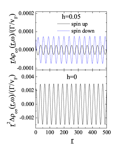
One can verify that the leading asymptotic behavior at large $r$ gives vanishing contributions to the LDOS in the absence of magnetic field ( $h=0$ ), providing $r|\omega+\mu|/v_{F}\gg 1$ . In other words, the $1/r$ contribution in $t_{0\sigma}^{\text{hel}}(r,i\omega)$ is exactly cancelled by that in $t_{1}^{\text{hel}}(r,i\omega)$ . The next order of the asymptotic expansion gives rise to the $1/r^{2}$ behavior with oscillation, where its frequency is $2r(\omega+\mu)/v_{F}$ , i.e.

\displaystyle\Delta\rho_{c\sigma}^{\text{hel}}(r,\omega)\sim\sin(2r(\omega+\mu)/v_{F})/r^{2}.

When a weak magnetic field is switched on, the leading asymptotic in Eq. (55) maintains its non-vanishing contribution, corresponding to

\displaystyle\Delta\rho_{c\sigma}^{\text{hel}}(r,\omega)\sim\sin(2r(\omega+\mu)/v_{F})/r.

There are three sources which lead to the asymptotic $1/r$ . The first is $G_{f\sigma}(\omega)\not=G_{f,-\sigma}(\omega)$ . The second is the opening of an effective gap due to the magnetic field. The last is the opposite spin scattering contribution, given by $\sigma g^{\gamma}_{s,-s}(k,\omega)$ in Eq. (48). Then, the $1/r$ contribution in Eq. (48) does not cancel that of Eq. (49).

In Fig. 2 we plot $r^{\nu}\Delta\rho_{c\sigma}^{\text{hel}}(r,\omega)$ , where $\nu=2$ for $h=0$ , and $\nu=1$ for finite $h$ . The impurity Green’s function is calculated within the slave-boson mean-field approximation, described in the previous section. This plot confirms the above analysis for the asymptotic behavior of the LDOS at large distance $r$ . The LDOS exhibits the Friedel oscillation, where its decay changes from $1/r^{2}$ to $1/r$ when the magnetic field is switched on. The magnetic field distinguishes the asymptotic behavior of the LDOS unambiguously.

The local charge density can be found from Eq. (39)

\displaystyle n_{c}^{\text{hel}}(r)=n_{0\sigma}^{\text{hel}}+\Delta n_{c\sigma}^{\text{hel}}(r),

(56)

where $n_{0\sigma}^{\text{hel}}$ is the bare charge density of helical electrons, and $\Delta n_{c\sigma}^{\text{hel}}(r)$ is the local modulation of the helical-electron charge density due to the presence of an impurity. $\Delta n_{c\sigma}^{\text{hel}}(r)$ corresponds to the $\Delta\rho_{c\sigma}^{\text{hel}}(r,\omega)$ part in the LDOS. At large distance $r$ , we find that $\Delta n_{c\sigma}^{\text{hel}}(r)$ fits very well with the asymptotic expansion $\exp(-\xi r/v_{F})/r^{\nu}$ , where $\nu$ is the same power of the LDOS. $\xi$ is not a universal parameter, depending on the microscopic detail. In Fig. 3 we plot $r^{\nu}\exp(\xi r/v_{F})\Delta n_{c\sigma}^{\text{hel}}(r)$ as a function of $r$ . It shows that the local charge density also exhibits the Friedel oscillation, where its decay, apart from the relaxation part $\exp(-\xi r/v_{F})$ , also obeys the same power law as the LDOS.

In general, the LSDOS of helical electrons does not vanish. The $z$ -component of the LSDOS is basically the difference of the LDOS for up and down spins. It vanishes when magnetic field is absent. When the magnetic field is switched on, like the LDOS, the $z$ -component of the LSDOS also exhibits the Friedel oscillation and decays as $1/r$ at large distance $r$ . The local spin density $S^{z}_{c}(r)$ also has the asymptotic $\exp(-\xi r/v_{F})/r$ when the magnetic field is finite. The $x$ - and $y$ - components of the LSDOS are finite even in the absence of magnetic field as it should be.

III.3 Friedel oscillation in the soft-gap metal

One can calculate the LDOS of conduction electrons in the soft-gap metal, following the previous discussion in the helical metal. The electron Green’s function can be expressed in the $\gamma_{\sigma}$ basis of Hamiltonian (25)

	$\displaystyle G_{c\alpha\beta\sigma}^{\text{sg}}(\mathbf{k},\mathbf{k}^{\prime},\omega)\equiv\langle\langle c_{\mathbf{k}\beta\sigma}\|c^{\dagger}_{\mathbf{k}\alpha\sigma}\rangle\rangle_{\omega}$
	$\displaystyle=\frac{\Phi_{\alpha\beta}(\phi,\phi^{\prime})}{4\pi\sqrt{kk^{\prime}}}\sum\limits_{mm^{\prime}=0,-1}\sum\limits_{\delta\tau}e^{im\phi-im^{\prime}\phi^{\prime}}\eta_{\delta\tau}^{\alpha\beta}$
	$\displaystyle\langle\langle\gamma_{m\delta\sigma}(k)\|\gamma_{m^{\prime}\tau\sigma}^{\dagger}(k^{\prime})\rangle\rangle_{\omega}$
	$\displaystyle+\frac{\Phi_{\alpha\beta}(\phi,\phi^{\prime})}{4\pi k}\delta(k-k^{\prime})\sum\limits_{mm^{\prime}\not=0,-1}e^{im(\phi-\phi^{\prime})}$
	$\displaystyle\Big(\frac{1}{\omega+\mu_{\sigma}-v_{F}k}+\alpha\beta\frac{1}{\omega+\mu_{\sigma}+v_{F}k}\Big),$		(57)

where $\Phi_{\alpha\beta}(\phi,\phi^{\prime})=\exp[i(1-\alpha)\phi/2-i(1-\beta)\phi^{\prime}/2]$ and $\eta_{++}^{\alpha\beta}=1$ , $\eta_{+-}^{\alpha\beta}=\beta$ , $\eta_{-+}^{\alpha\beta}=\alpha$ , $\eta_{--}^{\alpha\beta}=\alpha\beta$ .

Using the equation of motion method, the $\gamma_{\sigma}$ Green’s function is expressed by the impurity Green’s function

	$\displaystyle\langle\langle\gamma_{m\delta\sigma}(k)\|\gamma_{m^{\prime}\tau\sigma}^{\dagger}(k^{\prime})\rangle\rangle_{\omega}=\delta(k-k^{\prime})\delta_{mm^{\prime}}\delta_{\delta\tau}g^{\gamma}_{\delta\sigma}(k,\omega)$
	$\displaystyle+\frac{N\|V\|^{2}}{4\pi}\sqrt{kk^{\prime}}\zeta_{m\delta}\zeta_{m^{\prime}\tau}g^{\gamma}_{\delta\sigma}(k,\omega)g^{\gamma}_{\tau\sigma}(k^{\prime},\omega)G_{f\sigma}(\omega),$		(58)

where $\zeta_{0+}=\zeta_{0-}=\zeta_{-1+}=-\zeta_{-1-}=1$ and

\displaystyle g_{\alpha\sigma}^{\gamma}(k,\omega)=\frac{1}{\omega+\mu_{\sigma}-\alpha\varepsilon_{k}}.

(59)

Inserting the conduction-electron Green’s function calculated by Eqs. (57)-(58) into Eq. (38), we obtain the LDOS

$\displaystyle\rho_{c\sigma}^{\text{sg}}(\mathbf{r},\omega)$	$\displaystyle=$	$\displaystyle i\sum_{\alpha}\sum_{\mathbf{k}\mathbf{k}^{\prime}}e^{i(\mathbf{k}-\mathbf{k}^{\prime})\cdot\mathbf{r}}[G^{\text{sg}}_{c\alpha\alpha\sigma}(\mathbf{k},\mathbf{k}^{\prime},\omega^{+})$	(60)
		$\displaystyle\hskip 65.44142pt-G^{\text{sg}}_{c\alpha\alpha\sigma}(\mathbf{k},\mathbf{k}^{\prime},\omega^{-})]$
	$\displaystyle=$	$\displaystyle\rho_{0\sigma}^{\text{sg}}(\omega)+\Delta\rho_{c\sigma}^{\text{sg}}(r,\omega),$

where

	$\displaystyle\rho_{0\sigma}^{\text{sg}}(\omega)=-\frac{1}{\pi}\text{Im}\int\limits_{0}^{\infty}dkkg_{c\sigma}^{\text{sg}}(k,\omega^{+}),\;\;\;\;$		(61)
	$\displaystyle\Delta\rho_{c\sigma}^{\text{sg}}(r,\omega)=-\frac{4\Gamma}{v_{F}}\text{Im}\Big[G_{f\sigma}(\omega^{+})\Big(\big(t_{0\sigma}^{\text{sg}}\big(r,\omega^{+}\big)\big)^{2}$
	$\displaystyle+\big(t_{1\sigma}^{\text{sg}}\big(r,\omega^{+}\big)\big)^{2}\Big)\Big].\;\;$		(62)

The functions $t_{0\sigma}^{\text{sg}}(r,\omega)$ and $t_{1\sigma}^{\text{sg}}(r,\omega)$ are given by

	$\displaystyle t_{0\sigma}^{\text{sg}}(r,\omega)$	$\displaystyle=$	$\displaystyle v_{F}\int\limits_{0}^{\infty}dkkJ_{0}(kr)\frac{1}{2}\sum_{\alpha}g^{\gamma}_{\alpha\sigma}(k,\omega),$		(63)
	$\displaystyle t_{1\sigma}^{\text{sg}}(r,\omega)$	$\displaystyle=$	$\displaystyle v_{F}\int\limits_{0}^{\infty}dkkJ_{1}(kr)\frac{1}{2}\sum_{\alpha}\alpha g^{\gamma}_{\alpha\sigma}(k,\omega),$		(64)

and the bare Green’s function of conduction electrons is

\displaystyle g_{c\sigma}^{\text{sg}}(k,\omega)=\sum_{\alpha}g^{\gamma}_{\alpha\sigma}(k,\omega).

(65)

Note that the magnetic field in the $z$ -direction does not cause spin flipping in the graphene, thus the gap opening does not occur, differentiated from the helical metal.

Using the Lorentzian cutoff [17] with $\Lambda$ , we obtain the $t$ -functions

	$\displaystyle t_{0\sigma}^{\text{sg}}(r,i\omega)=-\frac{2}{\pi}\frac{\Lambda(i\omega+\mu_{\sigma})}{\Lambda^{2}-(\omega-i\mu_{\sigma})^{2}}$
	$\displaystyle\times\big[K_{0}\big(\frac{r}{v_{F}}(\omega-i\mu_{\sigma})\big)-K_{0}\big(\frac{r}{v_{F}}\Lambda\big)\big],$		(66)
	$\displaystyle t_{1\sigma}^{\text{sg}}(r,i\omega)=-\frac{2}{\pi}\frac{\Lambda}{\Lambda^{2}-(\omega-i\mu_{\sigma})^{2}}$
	$\displaystyle\times\big[(\omega-i\mu_{\sigma})K_{1}\big(\frac{r}{v_{F}}(\omega-i\mu_{\sigma})\big)-\Lambda K_{1}\big(\frac{r}{v_{F}}\Lambda\big)\big].$		(67)

One can verify that the leading order in the asymptotic expansion of the modified Bessel function in Eq. (55) gives vanishing contributions to the LDOS for any values of $h$ . The next order of the asymptotic expansion leads to $\Delta\rho_{c\sigma}^{\text{sg}}\sim\sin(2r(\omega+\mu_{\sigma})/v_{F})/r^{2}$ . This situation is exactly the same as the intranodal scattering in graphene.[23] In the present model we take into account only one Dirac cone, thus internodal scattering is not introduced. It was demonstrated that the $1/r$ behavior can originate from the internodal scattering between two different valleys in graphene. The inter-valley scattering gives rise to pseudospin mixing, resulting in the $1/r$ behavior. In the helical metal the magnetic field gives rise to spin flipping, allowing the $1/r$ law.

In Fig. 4 we plot $r^{2}\Delta\rho_{c\sigma}^{\text{sg}}(r,\omega)$ , where the impurity Green’s function is based on the slave-boson mean-field analysis. This plot confirms the $1/r^{2}$ decay of the LDOS, independent on the magnetic field. In particular, we point out $t_{n}^{\text{hel}}(r,\omega)=t_{n}^{\text{sg}}(r,\omega)$ in the absence of magnetic field, explicitly verified from Eqs. (53)-(54) and (66)-(67), resulting in the completely same Friedel oscillation for both helical and graphene cases. One may regard that this equivalence originates from the identical effective impurity action for both helical and graphene cases without the magnetic field. On the other hand, the magnetic field leads the oscillation frequency of the $\downarrow$ spin to differ from that of the $\uparrow$ spin, where the period difference is proportional to the magnetic field strength, an important different point from the helical metal.

We also calculate the local charge density of soft-gap electrons. In Fig. 5 we plot $r^{\nu}\exp(\xi r/v_{F})\Delta n_{c\sigma}^{\text{sg}}(r)$ , where $\nu=2$ , and $\xi$ is an asymptotic fitting parameter. It confirms the asymptotic behavior of the local charge density as $\exp(-\xi r/v_{F})/r^{\nu}$ . As the LDOS, the decay of the local charge density always obeys the inverse-square law independently on magnetic field, apart from the relaxation part $\exp(-\xi r/v_{F})$ .

The $z$ -component LSDOS also vanishes in the absence of magnetic field as the helical metal. When the magnetic field is turned on, the $z$ -component of the LSDOS also decays as $1/r^{2}$ at large distance $r$ . Since the Friedel oscillations in the LDOS for up and down spins have different periods, it should exhibit amplitude modulation, not shown in the helical metal. One can show that $S^{z}_{c}(r)$ obeys the asymptotic expression $\exp(-\xi r/v_{F})/r^{2}$ for finite magnetic fields while the other components always vanish, different from the helical metal.

One may ask why the Friedel oscillation reflects spin or pseudospin physics although it is basically involved with charge dynamics. The underlying mechanism is the coupling between the orbital motion of charge degrees of freedom and spin or pseudospin dynamics. To control spin dynamics with magnetic field changes the orbital motion of charge, or to modify charge dynamics by electric field governs the spin dynamics via the spin-orbit coupling physics. This is one of the main research directions in the present condensed matter physics.

IV Discussion and Summary

In this paper we investigated the Kondo effect and the associated Friedel oscillation on the surface of the topological insulator, where spins are locked along the momentum direction. In particular, we examined the role of magnetic field $h$ to distinguish the Kondo effect and Friedel oscillation of the helical metal from those of the graphene metal, where pseudospins are locked along the momentum direction. It turns out that both the Kondo effect and Friedel oscillation of the helical metal are completely identical to those of the standard soft-gap Anderson model in the absence of magnetic field. However, the magnetic field was shown to play a different role for each case.

We found that the spin $\uparrow$ and $\downarrow$ splitting energy of the Kondo peak does not follow the typical $h$ -linear behavior of the soft-gap Anderson model. We revealed its physical origin and derived the analytic expression. In addition, we showed that the Friedel oscillation of the helical metal changes from the typical $1/r^{2}$ law associated with the Dirac spectrum to the $1/r$ behavior, applying magnetic field in the $z$ -direction while it still remains as $1/r^{2}$ in the graphene case. We clarified physics behind this change that magnetic field gives rise to spin mixing between $\uparrow$ and $\downarrow$ in the helical metal, resulting in gap. We pointed out that this mechanism is quite analogous to the internodal scattering in the graphene case, [23] introducing the pseudospin flipping. We propose the Kondo effect and Friedel oscillation as the fingerprint for the surface state of the topological insulator, measurable by Fourier transformation scanning tunneling spectroscopy.[19, 20, 21, 22]

An interesting issue not discussed in this study is on Ruderman-Kittel-Kasuya-Yosida (RKKY) correlations. It was demonstrated based on the variational wave-function approach that the spin-orbital quenching results in anisotropy for spin dynamics, leading spin correlations of the topological surface different from those of graphene which are SU(2) symmetric.[24] This nontrivial spin dynamics in the topological surface gives an interesting problem. Increasing magnetic impurities, which kinds of spin dynamics will appear as a competition between the Kondo effect and RKKY correlation? This research direction opens a novel window for the interplay among interactions (Kondo and RKKY), disorder, and topology.[28, 29, 30]

Acknowledgements.

We would like to thank T. Takimoto for useful discussions. We acknowledge the Korea Ministry of Education, Science and Technology (MEST) for the grant of the National Research Foundation of Korea (No. 2010-0074542) at the Asia Pacific Center for Theoretical Physics. M.-T. was also supported by the National Foundation for Science and Technology Development (NAFOSTED) of Vietnam.

Appendix A Comment on the unitary transformation

We consider another choice of the unitary transformation. [24, 25] The helical electron Hamiltonian (2) can be diagonalized by the unitary transformation

\displaystyle\hat{U}(\phi)=\frac{1}{\sqrt{2}}\left(\begin{array}[c]{cc}e^{-i\phi/2}&e^{-i\phi/2}\\ e^{i\phi/2}&-e^{i\phi/2}\end{array}\right).

This unitary transformation matrix has its period $4\pi$ , and the Berry phase $\pi$ is acquired when an electron encircles the Fermi surface. It has been chosen to study the Kondo effect in the helical metal, based on the variational method. [24]

Proceeding in a similar way as in Sec. II, we obtain

\displaystyle H^{c}_{\text{hel}}=\sum\limits_{m\sigma}\int\limits_{0}^{\infty}dk\varepsilon_{k}\sigma\gamma_{m\sigma}^{\dagger}(k)\gamma_{m\sigma}(k).

(71)

The hybridization Hamiltonian becomes

\displaystyle H_{\text{hel}}^{\text{hyb}}=\frac{\sqrt{N}V}{\sqrt{2\pi}}\sum\limits_{m\sigma s}\int\limits_{0}^{\infty}dk\sqrt{k}f_{\sigma}^{\dagger}\xi_{\sigma s}(m)\gamma_{ms}(k)+\text{H.c.},\hskip 14.22636pt

(72)

where

\displaystyle\hat{\xi}(m)=\left(\begin{array}[c]{cc}\xi_{m}^{-}&\xi_{m}^{-}\\ \xi_{m}^{+}&-\xi_{m}^{+}\end{array}\right)

and

\displaystyle\xi^{\pm}_{m}=\frac{\sqrt{2}}{\pi}\frac{i}{2m\pm 1}.

It should be noted that the hybridization Hamiltonian in this $\gamma_{\sigma}$ basis couples the impurity for all angular momentum $m$ , much different from the case of the helical metal.

We introduce new operators for diagonalization

\displaystyle\psi_{m\pm}(k)=\frac{1}{\sqrt{2}}(\gamma_{m\uparrow}(k)\pm\gamma_{m\downarrow}(k)).

(76)

Then, the Hamiltonian (1) is written as follows

$\displaystyle H_{\text{hel}}$	$\displaystyle=$	$\displaystyle\sum\limits_{m}\int\limits_{0}^{\infty}dk\varepsilon_{k}[\psi_{m+}^{\dagger}(k)\psi_{m-}(k)+\psi_{m-}^{\dagger}(k)\psi_{m+}(k)]$	(77)
	$\displaystyle-$	$\displaystyle\sum\limits_{m\sigma}\int\limits_{0}^{\infty}dk\mu_{\sigma}\psi_{m\sigma}^{\dagger}(k)\psi_{m\sigma}(k)$
	$\displaystyle+$	$\displaystyle\sum\limits_{\sigma}E_{f\sigma}f_{\sigma}^{\dagger}f_{\sigma}+Un_{\uparrow}^{f}n_{\downarrow}^{f}$
	$\displaystyle+$	$\displaystyle\frac{\sqrt{N}V}{\sqrt{\pi}}\sum\limits_{m\sigma}\int\limits_{0}^{\infty}dk\sqrt{k}f_{\sigma}^{\dagger}\xi_{m}^{-\sigma}\psi_{m\sigma}(k)+\text{H.c.}$

Integrating over the $\psi_{\sigma}$ field, we obtain the effective impurity action

	$\displaystyle S_{\text{hel}}$	$\displaystyle=$	$\displaystyle\sum\limits_{\sigma\sigma^{\prime}}\int\limits_{0}^{\beta}d\tau f_{\sigma}^{\dagger}(\tau)[\delta_{\sigma\sigma^{\prime}}\delta(\tau-\tau^{\prime})(\partial_{\tau}+E_{f\sigma})$		(78)
		$\displaystyle+$	$\displaystyle\tilde{\Delta}_{\sigma\sigma^{\prime}}(\tau-\tau^{\prime})]f_{\sigma^{\prime}}(\tau^{\prime})+U\int\limits_{0}^{\beta}d\tau n_{\uparrow}^{f}(\tau)n_{\downarrow}^{f}(\tau),\hskip 22.76228pt$		(78)

where

\displaystyle\tilde{\Delta}_{\sigma\sigma^{\prime}}(i\omega)=\frac{N|V|^{2}}{\pi}\sum_{m}\int\limits_{0}^{\infty}dkk\tilde{g}_{\sigma\sigma^{\prime}}(k,i\omega)\xi_{m}^{-\sigma}(\xi_{m}^{-\sigma^{\prime}})^{*},\hskip 14.22636pt

(79)

and

\displaystyle\tilde{g}_{\sigma\sigma^{\prime}}(k,i\omega)=\left(\begin{array}[]{cc}i\omega+\mu+h&\varepsilon_{k}\\ \varepsilon_{k}&i\omega+\mu-h\end{array}\right)^{-1}_{\sigma\sigma^{\prime}}.

Calling $\sum_{m}\xi_{m}^{-\sigma}(\xi_{m}^{-\sigma^{\prime}})^{*}=\delta_{\sigma\sigma^{\prime}}/2$ , we obtain

\displaystyle\tilde{\Delta}_{\sigma\sigma^{\prime}}(i\omega)=\delta_{\sigma\sigma^{\prime}}\Delta_{\sigma}^{\text{hel}}(i\omega).

(83)

Thus, the effective action [Eq. (78)] is completely identical to the one [Eq. (21)].

The reason why the single-valuedness of the unitary transformation is not relevant for impurity dynamics may be the fact that the Berry phase contribution is integrated out, not affecting the local dynamics. Then, the feedback effect of the impurity dynamics to conduction electrons may be modified by the double-valued unitary transformation. Actually, all angular-momentum channels are coupled to the impurity. This will be addressed near future.

References

[1] M. Z. Hasan and C. L. Kane, arXiv:1002.3895 (unpublished); M. Konig, H. Buhmann, L. W. Molenkamp, T. Hughes, C.-X. Liu, X.-L. Qi, and S.-C. Zhang, J. Phys. Soc. Jpn. 77, 031007 (2008); S. Murakami, Prog. Theor. Phys. Suppl. 176, 279 (2008).
[2] S. Bieri and J. Frohlich, arXiv:1006.0457 (unpublished).
[3] F. D. M. Haldane, Phys. Rev. Lett. 61, 2015 (1988).
[4] C. L. Kane and E. J. Mele, Phys. Rev. Lett. 95, 146802 (2005).
[5] L. Fu, C. L. Kane, and E. J. Mele Phys. Rev. Lett. 98, 106803 (2007).
[6] J. E. Moore and L. Balents, Phys. Rev. B 75, 121306 (2007).
[7] R. Roy, Phys. Rev. B 79, 195322 (2009); R. Roy, Phys. Rev. B 79, 195321 (2009).
[8] H. Zhang, C. X. Liu, X. L. Qi, X. Dai, Z. Fang, and S. C. Zhang, Nature Physics 5, 438 (2009).
[9] S. Ryu, C. Mudry, H. Obuse, and A. Furusaki, Phys. Rev. Lett. 99, 116601 (2007).
[10] X.-L. Qi, R. Li, J. Zang, S.-C. Zhang, Science 323, 1184 (2009); R. Li, J. Wang, X.-L. Qi, S.-C. Zhang, Nature Physics 6, 284 (2010); R. Yu, W. Zhang, H.-J. Zhang, S.-C. Zhang, X. Dai, and Z. Fang, Science [DOI: 10.1126/science.1187485].
[11] J. Moore, Nature Physics 5, 378 (2009); A. M. Essin, J. E. Moore, D. Vanderbilt, Phys. Rev. Lett. 102, 146805 (2009).
[12] D. Hsieh, D. Qian, L. Wray, Y. Xia, Y. S. Hor, R. J. Cava, and M. Z. Hasan, Nature 452, 970 (2008).
[13] D. Hsieh, Y. Xia, L. Wray, D. Qian, A. Pal, J. H. Dil, J. Osterwalder, F. Meier, G. Bihlmayer, C. L. Kane, Y. S. Hor, R. J. Cava, and M. Z. Hasan, Science 323, 919 (2009).
[14] D. Hsieh, Y. Xia, D. Qian, L. Wray, J. H. Dil, F. Meier, J. Osterwalder, L. Patthey, J. G. Checkelsky, N. P. Ong, A. V. Fedorov, H. Lin, A. Bansil, D. Grauer, Y. S. Hor, R. J. Cava and M. Z. Hasan, Nature 460, 1101 (2009).
[15] Y. L. Chen, J. G. Analytis, J.-H. Chu, Z. K. Liu, S.-K. Mo, X. L. Qi, H. J. Zhang, D. H. Lu, X. Dai, Z. Fang, S. C. Zhang, I. R. Fisher, Z. Hussain, and Z.-X. Shen, Science 325, 178 (2009).
[16] J. J. Cha, J. R. Williams, D. Kong, S. Meister, H. Peng, A. J. Bestwick, P. Gallagher, D. Goldhaber-Gordon, and Y. Cui, Nano Lett. 10, 1076 (2010).
[17] C. R. Cassanello and E. Fradkin, Phys. Rev. 53, 15079 (1996).
[18] A. H. C. Neto, F. Guinea, N. M. R. Peres, K. S. Novoselov, and A. K. Geim, Rev. Mod. Phys. 81, 109 (2009).
[19] P. Mallet, F. Varchon, C. Naud, L. Magaud, C. Berger, and J.-Y. Veuillen, Phys. Rev. B 76, 041403(R) (2007).
[20] G. M. Rutter, J. N. Crain, N. P. Guisinger, T. Li, P. N. First, J. A. Stroscio, Science 317, 219 (2007).
[21] F. Vonau, D. Aubel, G. Gewinner, S. Zabrocki, J. C. Peruchetti, D. Bolmont, and L. Simon, Phys. Rev. Lett. 95, 176803 (2005).
[22] E. Dupont-Ferrier , P. Mallet , L. Magaud and J. Y. Veuillen , Europhys. Lett. 72, 430 (2005).
[23] C. Bena, Phys. Rev. Lett. 100, 076601 (2008).
[24] X.-Y. Feng, W.-Q. Chen, J.-H. Gao, Q.-H. Wang, and F.-C. Zhang, Phys. Rev. B 81, 235411 (2010).
[25] R. Zitko, Phys. Rev. B 81, 241414 (2010).
[26] N. Read and D. M. Newns, J. Phys. C: Solid State Phys. 16, L1055 (1983).
[27] Handbook of Mathematical Functions with Formulas, Graphs, and Mathematical Tables, ed. by M. Abramowitz and I. A. Stegun, Dover Publications, New York (1972).
[28] M. Dzero, K. Sun, V. Galitski, and P. Coleman, Phys. Rev. Lett. 104, 106408 (2010).
[29] K. Dhochak, R. Shankar, and V. Tripathi, Phys. Rev. Lett. 105, 117201 (2010).
[30] Minh-Tien Tran and Ki-Seok Kim, Phys. Rev. Lett. 105, 116403 (2010).