Decoding of Convolutional Codes
over the Erasure Channel

Virtudes Tomás Joachim Rosenthal Roxana Smarandache ^†^†thanks: V. Tomás is with the Department of Computational Science and Artificial Intelligence University of Alicante Alicante, Spain. (e-mail: vtomas@dccia.ua.es). Her research has been supported by Spanish grant MTM2008-06674-C02-01 and a grant of the Vicerectorat d’Investigació, Desenvolupament i Innovació of the Universitat d’Alacant for PhD students during a stay at Zürich Universität on charge to the same program. ^†^†thanks: J. Rosenthal is with the Mathematics Institute, University of Zürich, Winterthurerstr 190, CH-8057 Zürich, Switzerland. (www.math.uzh.ch/aa). His research was supported in part by the Swiss National Science Foundation under Project no. 126948.^†^†thanks: R. Smarandache is with the Department of Mathematics and Statistics, San Diego State University, San Diego, CA 92182-7720, USA. (e-mail: rsmarand@sciences.sdsu.edu). Her research is supported in part by by NSF Grants DMS-0708033 and TF-0830608.^†^†thanks: Part of these results where presented in the 2009 IEEE International Symposium on Information Theory in Seoul, Korea˜[31] and the 2010 International Symposium on Mathematical Theory of Networks and Systems˜[32].

Abstract

In this paper the decoding capabilities of convolutional codes over the erasure channel are studied. Of special interest will be maximum distance profile (MDP) convolutional codes. These are codes which have a maximum possible column distance increase.

It is shown how this strong minimum distance condition of MDP convolutional codes help us to solve error situations that maximum distance separable (MDS) block codes fail to solve. Towards this goal, two subclasses of MDP codes are defined: reverse-MDP convolutional codes and complete-MDP convolutional codes. Reverse-MDP codes have the capability to recover a maximum number of erasures using an algorithm which runs backward in time. Complete-MDP convolutional codes are both MDP and reverse-MDP codes. They are capable to recover the state of the decoder under the mildest condition. It is shown that complete-MDP convolutional codes perform in many cases better than comparable MDS block codes of the same rate over the erasure channel.

Index Terms:

Convolutional codes, maximum distance separable (MDS) block codes, decoding, erasure channel, maximum distance profile (MDP) convolutional codes, reverse-MDP convolutional codes, complete-MDP convolutional codes.

1 Introduction

When transmitting over an erasure channel like the Internet, one of the problems encountered is the delay experienced on the received information due to the possible re-transmission of lost packets. One way to eliminate these delays is by using forward error correction. Until now mainly block codes have been used for such a task, see, e.g., [3, 14] and the references therein. The use of convolutional codes over the erasure channel has been studied much less. We are aware of the work of Epstein [2] and of the more recent work by Arai et al. [1]. In this paper, we define a class of convolutional codes with strong distance properties, which we call complete maximum distance profile (complete-MDP) convolutional codes, and we demonstrate how they provide an attractive alternative.

The advantage that convolutional codes have over block codes, which will be exploited in our algorithms, is the flexibility obtained through the “sliding window” characteristic of convolutional codes. The received information can be grouped in appropriate ways, depending on the erasure bursts, and then be decoded by decoding the “easy” blocks first. This flexibility in grouping information brings certain freedom in the handling of sequences; we can split the blocks in smaller windows, we can overlap windows and we can proceed to decode in a less strict order. The blocks are not fixed as in the block code case, i.e., they do not have a fixed grouping of a fixed length. We can slide along the transmitted sequence and decide the place where we want to start our decoding. In other words, we can adapt the process to the pattern of erasures we receive. With this “sliding window” property of convolutional codes, together with the extra algebraic properties of maximum distance profile (MDP) convolutional codes, we are able to correct in a given block more erasures than a block code of that same length could do.

An $[N,K]$ block code used for transmission over an erasure channel can correct up to $N-K$ erasures in a given block, with the optimal error capability of $N-K$ being achieved by an $[N,K]$ maximum distance separable (MDS) code.

As an alternative, consider now a class of $(n,k,\delta)$ convolutional codes, i.e., a class of rate $k/n$ convolutional codes having degree $\delta$ . We will demonstrate that for this class, the maximum number of errors which can be corrected in some sliding window of appropriate size is achieved by the subclass of MDP convolutional codes. Moreover, we give examples of situations where the MDP code can recover patterns of erasures that cannot be decoded by an MDS block code of the same rate. In addition, we can increase further the recovering capability of MDP codes by imposing certain extra algebraic conditions and thus defining a subclass of MDP convolutional codes, called reverse maximum distance profile (reverse-MDP) convolutional codes. These codes allow an inversion of the direction of the decoding from right-to-left. Due to this fact one can recover through a backward process more erasures than with an MDP code. Following the definition and explanation of their advantages, we will prove the existence of the reverse-MDP codes and give a particular construction as well as a procedure to compute the so called reverse-superregular matrices necessary to build them.

As a final step we add stronger and more restrictive conditions to our codes in order to achieve an optimum performance of the recovering process. We obtain what we call complete-MDP convolutional codes. These codes help reducing the waiting time necessary when a large burst of erasures occurs and no correction is possible for a while. Simulations results show that these codes can decode extremely efficiently when compared to MDS block codes. Thus, they provide a very attractive choice when transmitting over an erasure channel.

MDP convolutional codes were first introduced in [10]. The usefulness of the MDP property when transmitting over the erasure channel was first recognized by the authors in two conference papers [31, 32]. The concept of complete MDP convolutional codes was first introduced by the first author in her dissertation [30]. The results we present here are an extension of [30].

Because of the increasing importance of packet switched networks the need to develop coding techniques for the erasure channel has gained a lot of importance. On the side of block codes and convolutional codes of a fixed rate there have been important studies done using so called “rateless erasure codes”. These codes were first introduced by Luby [17] and an important refinement was done by Shokrollahi who introduced so called Raptor codes [28]. In this paper we will not make a performance comparison of MDP codes with rateless erasure codes.

The paper is organized as follows. Section 2 provides the necessary background for the development of the paper: Subsection 2-A explains the assumptions on the channel model, and Subsection 2-B provides all the necessary concepts about convolutional codes, MDP convolutional codes and their characterizations. Section 3 illustrates our proposed decoding algorithm over the erasure channel. It also presents examples and special concerns to be addressed when comparing them with MDS block codes. In Section 4, we introduce the idea of backwards decoding process and we define and prove the existence of reverse-MDP convolutional codes as codes able to do this. In Section 5, we give a method to construct these codes and in Subsection 5-A, we explain how to construct a special kind of matrices necessary in order to build reverse-MDP convolutional codes. Section 6 introduces the concept of complete-MDP convolutional codes and shows how these codes can help to reduce the waiting time in the recovering process. In Subsection 6-A we provide simulation result assuming a Gilbert-Elliot channel model. It is shown that for equal rate and chosen degrees comparable to chosen block length the performance of complete-MDP codes are a better option than MDS block codes.

In Section 7 we provide theoretical results which compare MDS block codes with MDP convolutional codes. The main result shows that both a rate $k/n$ MDS block code as well as a $k/n$ MDP convolutional code can decode erasures at a rate of $(n-k)/n$ in average. For the MDS block code error free communication is possible if at most $n-k$ erasures happen in every block. For the MDP convolutional code error free communication is possible if the number of erasures per sliding window, whose size depends on the degree, is not larger than a certain amount.

2 Preliminaries

This section contains the necessary mathematical background and the channel assumptions needed for the development of our results. Note that throughout the paper vectors of length $n$ over a field $\mathbb{F}$ will be viewed as $n\times 1$ matrices, i.e., as column vectors.

2-A Erasure channel

An erasure channel is a communication channel where the symbols sent either arrive correctly or they are erased; the receiver knows that a symbol has not been received or was received incorrectly. An important example of an erasure channel is the Internet, where packet sizes are upper bounded by 12,000 bits - the maximum that the Ethernet protocol allows (that everyone uses at the user end). In many cases, this maximum is actually used [4]. Due to the nature of the TCP part of the TCP/IP protocol stack, most sources need an acknowledgment confirming that the packet has arrived at the destination; these packets are only 320 bits long. So if everyone were to use TCP/IP, the packet size distribution would be as follows: 35% –320 bits, 35% – 12,000 bits and 30% – uniform distribution in between the two. Real-time traffic used, e.g., in video calling, does not need an acknowledgment since that would take too much time; overall, the following is a good assumption of the packet size distribution: 30% – 320 bits, 50% – 12,000 bits, 20% –uniform distribution in between, see [29] and [15, Table II].

We can model each packet as an element or sequence of elements from a large alphabet. Packets sent over the Internet are protected by a cyclic redundancy check (CRC) code. If the CRC check fails, the receiver knows that a packet is in error or has not arrived [21]; it then declares an erasure. Undetected errors are rare and are ignored. For illustration purpose we employ as alphabet the finite field $\mathbb{F}:=\mathbb{F}_{2^{1,000}}$ . If a packet has less than 1,000 bits, then one uses simply the corresponding element of $\mathbb{F}$ . If the packet is larger, one uses several alphabet symbols to describe the packet. With or without interleaving, such an encoding scheme results in the property that errors tend to occur in bursts, and this is a phenomenon observed about many channels modeled via the erasure channel. This point is important to keep in mind when designing codes which are capable of correcting many errors over the erasure channel.

2-B Convolutional codes

Let $\mathbb{F}$ be a finite field. We view a convolutional code $\mathcal{C}$ of rate $k/n$ as a submodule of $\mathbb{F}[z]^{n}$ (see [7, 24, 23]) that can be described as

\mathcal{C}=\left\{\text{$v$}(z)\in\mathbb{F}[z]^{n}\ |\ \text{$v$}(z)=G(z)\text{$u$}(z)\ \text{with}\ \text{$u$}(z)\in\mathbb{F}[z]^{k}\right\},

where $G(z)$ is an $n\times k$ full-rank polynomial matrix called a generator matrix for $\mathcal{C}$ , $\text{$u$}(z)$ is an information vector, and $\text{$v$}(z)$ is the resulting code vector or the codeword.

The maximum degree of all polynomials in the $j$ -th column of $G(z)$ is called the $j$ -th column degree of $G(z)$ , and we denote it by $\delta_{j}$ .

We define the degree $\delta$ of a convolutional code $\mathcal{C}$ as the maximum of the degrees of the determinants of the $k\times k$ sub-matrices of one and hence any generator matrix of $\mathcal{C}$ . We say that $\mathcal{C}$ is an $(n,k,\delta)$ convolutional code [19].

Assume the $j$ -th column of $G(z)$ has degree $\delta_{j}$ . The high order coefficients matrix of $G(z)$ , $G_{\infty}$ , is the matrix whose $j$ -th column is formed by the coefficients of $z^{\delta_{j}}$ in the $j$ -th column of $G(z)$ . If $G_{\infty}$ has full rank, then $G(z)$ is called a minimal generator matrix and the degree $\delta$ of the code agrees in this situation with the overall constraint length (see [12, Section 2.5]) of the encoder $G(z)$ . Note that in this case $\delta=\sum_{i=1}^{k}\delta_{i}$ . Finally we define the memory of an encoder $G(z)$ as the maximum of the column degrees $\{\delta_{1},\ldots,\delta_{k}\}$ . This is the parameter of an encoder. When we choose however a minimal generator matrix then the memory becomes the property of the convolutional code.

We say that a code $\mathcal{C}$ is observable (see, e.g., [26, 23]) if the generator matrix $G(z)$ has a polynomial left inverse. This avoids the type of catastrophic situations in which a sequence $\text{$u$}(z)$ with an infinite number of nonzero coefficients can be encoded into a sequence $\text{$v$}(z)$ with a finite number of nonzero coefficients; this case would decode finitely many errors on the received code sequence into infinitely many errors when recovering the original information sequence. Therefore, only observable codes are regularly considered; therefore, these will be the codes on which we will focus our attention.

If $\mathcal{C}$ is an observable code, then it can be equivalently described using an $(n-k)\times n$ full rank polynomial parity-check matrix $H(z)$ , such that

\mathcal{C}=\left\{\text{$v$}(z)\in\mathbb{F}[z]^{n}\ \ |\ \ H(z)\text{$v$}(z)=\text{$0$}\in\mathbb{F}[z]^{n-k}\right\}.

If we write $\text{$v$}(z)=\mathbf{v}_{0}+\mathbf{v}_{1}z+\ldots+\mathbf{v}_{l}z^{l}$ , (with $l\geq 0$ ), and we represent $H(z)$ as a matrix polynomial,

H(z)=H_{0}+H_{1}z+\cdots+H_{\nu}z^{\nu},

where $H_{i}=O$ , for $i>\nu$ , we can expand the kernel representation in the following way

\displaystyle\left[\begin{array}[]{ccccc}H_{0}&\\ \vdots&\ddots&\\ H_{\nu}&\cdots&H_{0}\\ &\ddots&&\ddots\\ &&H_{\nu}&\cdots&H_{0}\\ &&&\ddots&\vdots\\ &&&&H_{\nu}\\ \end{array}\right]\left[\begin{array}[]{c}\mathbf{v}_{0}\\ \mathbf{v}_{1}\\ \vdots\\ \mathbf{v}_{l}\end{array}\right]=\text{$0$}.

An important distance measure for convolutional codes is the free distance $d_{\mbox{\rm\tiny free}}$ defined as

\mbox{$d_{\mbox{\rm\tiny free}}$}(\mathcal{C}):=\min\left\{\operatorname{wt}(\text{$v$}(z))\ \ |\ \ \text{$v$}(z)\in\mathcal{C}\quad\text{and}\quad\text{$v$}(z)\neq\text{$0$}\right\}.

The following lemma shows the importance of the free distance as a performance measure of a code used over the erasure channel.

Lemma 2.1.

Let $\mathcal{C}$ be a convolutional code with free distance $d\stackrel{{\scriptstyle\text{def}}}{{=}}\mbox{$d_{\mbox{\rm\tiny free}}$}$ . If during the transmission at most $d-1$ erasures occur, then these erasures can be uniquely decoded. Moreover, there exist patterns of $d$ erasures which cannot be uniquely decoded.

Proof:

Let $\text{$v$}(z)=\mathbf{v}_{0}+\mathbf{v}_{1}z+\ldots+\mathbf{v}_{l}z^{l}$ be a received vector with $d-1$ erased symbols erased in positions $i_{1},\ldots,i_{d-1}$ . The homogeneous system (2-B) of $(\nu+l+1)(n-k)$ equations with $(l+1)n$ unknowns can be changed into an equivalent non-homogeneous system

\displaystyle\hat{H}\left[\begin{array}[]{c}v_{i_{1}}\\ v_{i_{2}}\\ \vdots\\ v_{i_{d-1}}\end{array}\right]=\mathbf{b}

of $(\nu+l+1)(n-k)$ equations with $d-1$ unknowns $v_{i_{1}},\ldots,v_{i_{d-1}}$ where $\hat{H}$ is a $(d-1)(n-k)\times(d-1)n$ sub-matrix of

H=\left[\begin{array}[]{ccccc}H_{0}&\\ \vdots&\ddots&\\ H_{\nu}&\cdots&H_{0}\\ &\ddots&&\ddots\\ &&H_{\nu}&\cdots&H_{0}\\ &&&\ddots&\vdots\\ &&&&H_{\nu}\\ \end{array}\right].

This non-homogeneous system (2-B) has a solution, because of the assumption that the channel allows only erasures. In addition, the columns of the system matrix are linearly independent, because $d=\mbox{$d_{\mbox{\rm\tiny free}}$}(\mathcal{C})$ , so the matrix $\hat{H}$ has full column rank. It follows from these two facts that the solution must be unique.

If on the other hand more than $d$ erasures happen, then the associated linear system of equations does not have a unique solution anymore. ∎

Rosenthal and Smarandache [25] showed that the free distance of an $(n,k,\delta)$ convolutional code must be upper bounded by

\displaystyle\mbox{$d_{\mbox{\rm\tiny free}}$}(\mathcal{C})\leq(n-k)\left(\left\lfloor\frac{\delta}{k}\right\rfloor+1\right)+\delta+1.

(18)

This bound is known as the generalized Singleton bound [25] since it generalizes in a natural way the Singleton bound for block codes (the case $\delta=0$ ). Moreover, an $(n,k,\delta)$ convolutional code is a maximum distance separable (MDS) code [25] if its free distance achieves the generalized Singleton bound.

Another important distance measure is the $j$ th column distance [12], $d_{j}^{c}(\mathcal{C})$ , given by the expression

d_{j}^{c}(\mathcal{C})=\min\left\{\operatorname{wt}(\mathbf{v}_{[0,j]}(z))\ \ |\ \ \text{$v$}(z)\in\mathcal{C}\ \ \text{and}\ \ \mathbf{v}_{0}\neq\text{$0$}\right\},

where $\mathbf{v}_{[0,j]}(z)=\mathbf{v}_{0}+\mathbf{v}_{1}z+\ldots+\mathbf{v}_{j}z^{j}$ represents the $j$ -th truncation of the codeword $\text{$v$}(z)\in\mathcal{C}$ . It is related to the free distance $\mbox{$d_{\mbox{\rm\tiny free}}$}(\mathcal{C})$ in the following way

\displaystyle\mbox{$d_{\mbox{\rm\tiny free}}$}(\mathcal{C})=\lim_{j\rightarrow\infty}d_{j}^{c}(\mathcal{C}).

(19)

The $j$ -th column distance is upper bounded [6, 10]

\displaystyle d_{j}^{c}(\mathcal{C})\leq(n-k)(j+1)+1,

(20)

and the maximality of any of the column distances implies the maximality of all the previous ones, i.e., if $d_{j}^{c}(\mathcal{C})=(n-k)(j+1)+1$ for some $j$ , then $d_{i}^{c}(\mathcal{C})=(n-k)(i+1)+1$ for all $i\leq j$ , see [6, 10]. The $(m+1)$ -tuple $(d_{0}^{c}(\mathcal{C}),d_{1}^{c}(\mathcal{C}),\ldots,d_{m}^{c}(\mathcal{C}))$ is called the column distance profile of the code [12].

Since no column distance can achieve a value greater than the generalized Singleton bound, there must exist an integer $L$ for which the bound (20) could be attained for all $j\leq L$ and it is a strict upper bound for $j>L$ ; this value is

\displaystyle L=\left\lfloor\frac{\delta}{k}\right\rfloor+\left\lfloor\frac{\delta}{n-k}\right\rfloor.

(21)

An $(n,k,\delta)$ convolutional code $\mathcal{C}$ with $d_{L}^{c}(\mathcal{C})=(n-k)(L+1)+1$ is called a maximum distance profile (MDP) code [6, 10]. In this case, every $d_{j}^{c}(\mathcal{C})$ for $j\leq L$ is maximal, so we can say that the column distances of MDP codes increase as rapidly as possible for as long as possible.

The following two theorems characterize algebraically all convolutional codes of a given $j$ th column distance $d$ , and hence also MDP convolutional codes. Assume that the parity-check matrix is given as $H(z)=\sum^{\nu}_{i=0}H_{i}z^{i}$ . For each $j>\nu$ , let $H_{j}=O$ and define:

\mathcal{H}_{j}=\left[\begin{array}[]{cccc}H_{0}&&&\\ H_{1}&H_{0}&&\\ \vdots&\vdots&\ddots&\\ H_{j}&H_{j-1}&\cdots&H_{0}\end{array}\right]\in\mathbb{F}^{(j+1)(n-k)\times(j+1)n},

(22)

for all $j\geq 0$ .

Theorem 2.2.

([6, Proposition 2.1]) Let $d\in\mathbb{N}$ . The following properties are equivalent.

(a)

$d^{c}_{j}=d$ ;
(b)

none of the first $n$ columns of $\mathcal{H}_{j}$ is contained in the span of any other $d-2$ columns and one of the first $n$ columns of $\mathcal{H}_{j}$ is in the span of some other $d-1$ columns of that matrix.

Let $G(z)=\sum_{i=0}^{m}G_{i}z^{i}$ , $G_{j}=O,$ for all $j>\nu$ , and

\mathcal{G}_{j}=\left[\begin{array}[]{cccc}G_{0}&G_{1}&\cdots&G_{j}\\ &G_{0}&\cdots&G_{j-1}\\ &&\ddots&\vdots\\ &&&G_{0}\end{array}\right],\text{~for all ~}j\geq 0.

(23)

Then, the MDP convolutional codes are characterized as follows:

Theorem 2.3.

([6, Theorem 2.4]) Let $\mathcal{G}_{j}$ and $\mathcal{H}_{j}$ be like in (23) and (22). Then the following are equivalent:

(a)

$d_{j}^{c}=(n-k)(j+1)+1$ ;
(b)

every $(j+1)k\times(j+1)k$ full-size minor of $\mathcal{G}_{j}$ formed from the columns with indices $1\leq t_{1}<\cdots<t_{(j+1)k}$ , where $t_{sk+1}>sn$ , for $s=1,2,\ldots,j$ , is nonzero;
(c)

every $(j+1)(n-k)\times(j+1)(n-k)$ full-size minor of $\mathcal{H}_{j}$ formed from the columns with indices $1\leq r_{1}<\cdots<r_{(j+1)(n-k)}$ , where $r_{s(n-k)}\leq sn$ , for $s=1,2,\ldots,j$ , is nonzero.

In particular, when $j=L$ , $\mathcal{C}$ is an MDP convolutional code.

A code satisfying the conditions of Theorem 2.3 is said to have the MDP property.

Note that MDP convolutional codes are similar to MDS block codes within windows of size $(L+1)n$ . Indeed, the nonsingular full-size minors property given in the previous theorem ensures that if we truncate a codeword with its first nonzero component at any $j$ component, with $j\leq L$ , it will have weight higher or equal than the bound given in Theorem 2.3 (a), which is the Singleton bound for that block code.

3 Decoding over an erasure channel

Let us suppose that we use a convolutional code $\mathcal{C}$ to transmit over an erasure channel. Then we can state the following result.

Theorem 3.1.

Let $\mathcal{C}$ be an $(n,k,\delta)$ convolutional code with $d_{j_{0}}^{c}$ the $j_{0}$ -th column distance. If in any sliding window of length $(j_{0}+1)n$ at most $d_{j_{0}}^{c}-1$ erasures occur, then we can completely recover the transmitted sequence.

Proof:

Assume that we have been able to correctly decode up to an instant $t-1$ . Then we have the following homogeneous system:

\displaystyle\left[\begin{array}[]{cccccccccc}\!\!H_{\nu}&H_{\nu-1}&\cdots&H_{\nu-j_{0}}&\cdots&H_{0}\\ &H_{\nu}&\cdots&H_{\nu-j_{0}+1}&\cdots&H_{1}&H_{0}\\ &&\ddots&&&&&\ddots\\ &&&H_{\nu}&\cdots&H_{j_{0}}&H_{j_{0}-1}&\cdots&H_{0}\end{array}\right]\left[\begin{array}[]{c}\!\!\!\mathbf{v}_{t-\nu}\\ \!\!\!\vdots\\ \!\!\!\mathbf{v}_{t-1}\\ \!\!\!\star\\ \!\!\!\star\\ \!\!\!\vdots\\ \!\!\!\star\end{array}\right]=\text{$0$},

where $\star$ takes the place of a vector that had some of the components erased. Let the positions of the erased field elements be $i_{1},\ldots,i_{e},$ $e\leq d_{j_{0}}^{c}-1$ , where $i_{1},\ldots,i_{s},$ $s\leq n$ , are the erasures occurring in the first $n$ -vector erased. We can take the columns of the matrix in equation (3) that correspond to the coefficients of the erased elements to be the coefficients of a new system. The rest of the columns in (3) will help us to compute the independent terms. In this way we get a non-homogeneous system with $(j_{0}+1)(n-k)$ equations and $e\leq d_{j_{0}}^{c}-1$ , variables.

We claim that there is an extension $\{\mathbf{\tilde{v}}_{t},\ldots,\mathbf{\tilde{v}}_{t+j_{0}}\}$ such that the vector

(\mathbf{v}_{t-\nu},\ldots,\mathbf{v}_{t-1},\mathbf{\tilde{v}}_{t},\ldots,\mathbf{\tilde{v}}_{t+j_{0}})

is a codeword and such that $\mathbf{\tilde{v}}_{t}$ is unique.

Indeed, we know that a solution of the system exists since we assumed that only erasures occur. To prove the uniqueness of $\mathbf{\tilde{v}}_{t}$ , or equivalently, of the erased elements $\tilde{v}_{i_{1}},\ldots,\tilde{v}_{i_{s}},$ let us suppose there exist two such good extensions $\{\mathbf{\tilde{v}}_{t},\ldots,\mathbf{\tilde{v}}_{t+j_{0}}\}$ and $\{\mathbf{\tilde{\tilde{v}}}_{t},\ldots,\mathbf{\tilde{\tilde{v}}}_{t+j_{0}}\}$ . Let $\mathbf{h}_{i_{1}},\ldots,\mathbf{h}_{i_{e}}$ , be the column vectors of the sliding parity-check matrix in (3) which correspond to the erasure elements. We have: ~ v _i_1 h_i_1 + ⋯+ ~ v _i_sh_i_s+⋯+ ~ v _i_eh_i_e= ~ b and ~ ~ v _i_1 h_i_1 + ⋯+ ~ ~ v _i_sh_i_s + ⋯+ ~ ~ v _i_eh_i_e= ~ ~ b , where the vectors $\tilde{\mathbf{b}}$ and $\tilde{\tilde{\mathbf{b}}}$ correspond to the known part of the system. Subtracting these equations and observing that $\tilde{\mathbf{b}}=\tilde{\tilde{\mathbf{b}}}$ , we obtain: ( ~ v _i_1- ~ ~ v _i_1) h_i_1 + ⋯+( ~ v _i_s- ~ ~ v _i_s)h_i_s+⋯+ ( ~ v _i_e- ~ ~ v _i_e)h_i_e= $0$ . Using Theorem 2.2 part (b) we obtain that, necessarily,

\displaystyle\tilde{v}_{i_{1}}-

\displaystyle\tilde{\tilde{v}}_{i_{1}}=0,~\ldots,~\tilde{v}_{i_{s}}-\tilde{\tilde{v}}_{i_{s}}=0,

which proves the uniqueness of the solution.

In order to find the value of this unique vector, we solve the full column rank system, find a solution and retain the part which is unique. Then we slide $n$ bits to the next $n(j_{0}+1)$ window and proceed as above. ∎

The best scenario of Theorem 3.1 happens when the convolutional code is MDP. In this case, full error correction ‘from left to right’ is possible as soon as the fraction of erasures is not more than $\frac{n-k}{n}$ in any sliding window of length $(L+1)n$ .

Corollary 3.2.

Let $\mathcal{C}$ be an $(n,k,\delta)$ MDP convolutional code. If in any sliding window of length $(L+1)n$ at most $(L+1)(n-k)$ erasures occur in a transmitted sequence, then we can completely recover the sequence in polynomial time in $\delta$ by iteratively decoding the symbols ‘from left to right’.

Proof:

Under the given assumptions it is possible to compute one erasure after the other in a unique manner by processing ‘from left to right’. ∎

Remark 3.3.

The process of computing the erasures described in the proof of Theorem 3.1 leads to a natural algorithm. The computation of each erased symbol requires only simple linear algebra. In the optimum case of an MDP convolutional code, for every set of $(L+1)(n-k)$ erasures, a matrix of size at most $(L+1)(n-k)$ has to be inverted over the base field $\mathbb{F}$ . This is easily achieved even over fairly large fields. To be precise the number of elementary field operations is $\mathcal{O}\left(L^{3}(n-k)^{3}\right)$ and the most costly field operation in $\mathbb{F}_{q}$ , namely division, requires $\mathcal{O}\left(\log^{3}q\right)$ bit operations. $\square$

Remark 3.4.

Theorem 3.2 is optimal in the following sense. One can show that for any $(n,k,\delta)$ code there exist patterns of $(L+2)(n-k)$ erasures in a sliding window of length $(L+2)n$ which cannot be uniquely decoded.

In Corollary 7.2 we will show that the maximal recovering rate of any rate $k/n$ convolutional code over the erasure channel is at most $R=\frac{n-k}{n}$ . $\square$

Remark 3.5.

Although in Theorem 3.1 we fix the value $j=j_{0}$ , other window sizes can be taken during the decoding process in order to optimize it. For any value of $j$ , at most $d_{j}^{c}-1$ erasures can be recovered in a window of size $(j+1)n$ . In the MDP case, the parameter $L$ gives an upper bound on the length of the window we can take to correct. For every $j\leq L$ , in a window of size $(j+1)n$ we can recover at most $(j+1)(n-k)$ erasures. This means that we can conveniently choose the size of the window we need at each step depending on the distribution of the erasures in the sequence. This is an advantage of these codes over block codes. If we receive a part of sequence with a few errors we do not need to wait until we receive the complete block, we can already proceed with decoding within small windows relative to $L$ .

This property allows us to recover the erasures in situations where the MDS block codes cannot do it. The following example illustrates this scenario. We compare an MDP convolutional code with an MDS block code of the same length as the maximum window size taken for the convolutional code. $\square$

Example 3.6.

Consider a $(2,1,50)$ MDP convolutional code over an erasure channel. In this case, the decoding can be completed if in any sliding window of length $202$ not more than $101$ erasures occur; therefore, $50\%$ of the erasured components can be correctly recovered.

An MDS block code which can achieve a comparable performance is a $[202,101]$ MDS block code. In a block of $202$ symbols we can recover $101$ erased symbols, which is again $50\%$ error capability.

Suppose now that we have been able to correctly decode up to an instant $t$ . After time $t$ a new block of symbols starts whose start is indicated by $|$ . Assume now we receive the following pattern of erasures

\ldots\mathbf{v}\mathbf{v}|\overbrace{\star\star\ldots\star\star}^{(A)60}\overbrace{\mathbf{v}\mathbf{v}\ldots\mathbf{v}}^{(B)80}\overbrace{\star\star\ldots\star\star}^{(C)60}\mathbf{v}\mathbf{v}|\mathbf{v}\mathbf{v}\ldots,

where each $\star$ stands for a component of the vector that has been erased and $\mathbf{v}$ means that the component has been correctly received. In this situation, $120$ erasures happen in a block of $202$ symbols making the MDS block code unable to recover them. In the block code situation one has to skip the whole window and lose a whole block, and move to the next block.

The MDP convolutional code proves to be a better choice in this situation. If we frame a $120$ symbols length window, then in this window we can correct up to $60$ erasures. Let us frame a window containing the first $60$ erasures from $A$ and $60$ more correct symbols from $B$ . Note that following expression (3), in order to solve the corresponding system and to help us calculate the independent terms, we need to take the $100$ correct symbols that we decoded before receiving the block $A$ . In this way we can solve the system and recover the first block of $60$ erasures.

\overbrace{\mathbf{v}\mathbf{v}\ldots\mathbf{v}\mathbf{v}}^{100}|\overbrace{\star\star\ldots\star\star}^{(A)60}\overbrace{\mathbf{v}\mathbf{v}\ldots\mathbf{v}}^{(B)60}

Then we slide through the received sequence until we frame the rest of the erasures in a $120$ symbols window. As before, we make use of the $100$ previously decoded symbols to compute the independent terms of the system.

\overbrace{\mathbf{v}\mathbf{v}\ldots\mathbf{v}\mathbf{v}}^{(A+B)100}\overbrace{\star\star\ldots\star\star}^{(C)60}\overbrace{\mathbf{v}\mathbf{v}|\mathbf{v}\mathbf{v}\ldots}^{60}

After recovering this block we have correctly decoded the sequence. $\square$

Remark 3.7.

There are situations in which other patterns of erasures than the ones covered by Theorem 3.1 or Corollary 3.2 occur, and for which decoding within smaller window sizes than maximum allowed is not possible. This leads to an inability of correcting that block; we say that we are lost in the recovering process.

Looking at the following system of equations,

\displaystyle\left[\begin{array}[]{cccccccccc}H_{\nu}&H_{\nu-1}&\cdots&H_{\nu-j}&\cdots&H_{0}\\ &H_{\nu}&\cdots&H_{\nu-j+1}&\cdots&H_{1}&H_{0}\\ &&\ddots&&&&&\ddots\\ &&&H_{\nu}&\cdots&H_{j}&H_{j-1}&\cdots&H_{0}\end{array}\right]\left[\begin{array}[]{c}\!\!\!\mathbf{v}_{t-\nu}\\ \!\!\!\vdots\\ \!\!\!\mathbf{v}_{t}\\ \!\!\!\mathbf{v}_{t+1}\\ \!\!\!\vdots\\ \!\!\!\mathbf{v}_{t+j}\end{array}\right]=\text{$0$},

we see that, in order to continue our recovering process, we need to find a block of $\nu n$ correct symbols $\mathbf{v}_{t-\nu}$ to $\mathbf{v}_{t-1}$ preceding a block of $(j+1)n$ symbols $\mathbf{v}_{t}$ to $\mathbf{v}_{t+j}$ where not more than $d_{j}^{c}-1=(j+1)(n-k)$ erasures occur. In other words, we need to have some guard space, an expression often used in the literature. (See e.g. [5, p. 288] or [16, p. 430]). This allows a restart of the decoding algorithm leading to recovery of $\mathbf{v}_{t}$ to $\mathbf{v}_{t+j}$ .

In Section 6 we will derive Theorem 6.6 which provides somehow the weakest conditions possible which will guarantee the computation of a guard space once the decoder is lost in the decoding process.

We define the recovering rate per window as $R_{\omega}=\frac{\#\text{erasures recovered}}{\#\text{symbols in a window}}$ . Note that above condition of having a “guard space” and restarting the recovering process is a sufficient condition for $R_{\omega}$ to be maintained. For any generic $(n,k,\delta)$ convolutional code, $R_{\omega}=\frac{d_{j}^{c}-1}{(j+1)n}$ . In the MDP case where the number of possible recovered erasures is maximized, we have $R_{\omega}=\frac{(j+1)(n-k)}{(j+1)n}$ . $\square$

4 The backward process and the reverse-MDP convolutional codes

In this section we define a subclass of MDP codes, called reverse-MDP convolutional codes, which have the MDP property not only forward but also backward, i.e., if we truncate sequences $[\mathbf{v}_{0},\ldots,\mathbf{v}_{M}],$ $M\geq L$ , with $\mathbf{v}_{0}\neq\text{$0$}$ and $\mathbf{v}_{M}\neq\text{$0$}$ either at the beginning, to obtain $[\mathbf{v}_{0},\ldots,\mathbf{v}_{L}]$ , or at the end, to obtain $[\mathbf{v}_{M},\ldots,\mathbf{v}_{M-L}]$ , the minimum possible weight of the segments obtained is as large as possible. We will see in the following how this backward decoding ability of reverse-MDP codes makes these codes better choices than regular MDP convolutional codes for transmission over an erasure channel, since they can recover certain situations in which the latter would fail.

Example 4.1.

As previously, assume we use a $(2,1,50)$ MDP convolutional code to transmit over an erasure channel. Suppose that we are able to recover the sequence up to an instant $t$ , after which we receive a part of a sequence with the following pattern

\ldots\mathbf{v}\mathbf{v}\overbrace{\star\ldots\star}^{(A)22}\ \overbrace{\mathbf{v}\mathbf{v}\star\star\mathbf{v}\mathbf{v}\star\star\ldots\mathbf{v}\mathbf{v}\star\star}^{(B)180}\ |\overbrace{\mathbf{v}\mathbf{v}\ldots\mathbf{v}\mathbf{v}}^{(C)202}|

|\ \overbrace{\star\star\ldots\star}^{(D)80}\ \overbrace{\mathbf{v}\mathbf{v}\ldots\mathbf{v}}^{(E)62}\ \overbrace{\star\star\ldots\star}^{(F)60}\ |\ \overbrace{\mathbf{v}\mathbf{v}\ldots\mathbf{v}}^{(G)202},

where, as before, $\star$ means that the symbol has been erased, and $\mathbf{v}$ denotes a symbol has been correctly received. This is a situation in which we cannot recover the sequence by simply decoding ‘from left to right’ through the algorithm explained in remark 3.3. The simple ‘from left to right’ decoding algorithm for MDP convolutional codes needs to skip over these erasures, leading to the loss of this information. A $[202,101]$ MDS block code would not be a better choice either since in a block of $202$ symbols there would be more than $101$ erasures making that block undecodable. $\square$

This example shows that even with enough guard space between bursts of erasures, we cannot always decode if the bursts are too large relative to a given window. Let us imagine the following scenario. In the places where a guard space appears we change our decoding direction from left-to-right to right-to-left. Suppose that we could split the sequence into windows starting from the end, such that erasures are less accumulated in those windows, i.e., such that reading the patterns right-to-left would provide us with a distribution of erasures having an appropriate density per window to be recovered. Moreover, suppose that the code properties are such that inversion in the decoding direction is possible. Then, we would possibly increase the decoding capability leading to less information loss.

In order that such a scenario can work we should be able to compute a guard space (a sufficient large sequence of symbols without erasures). We will explain in Section 6 how this can be achieved.

We will refer to the left-to-right decoding process as forward decoding and to the inverted (from right-to-left) recovering process as backward decoding.

We will show how convolutional codes allow a “forward and backward flexibility” which, together with extra algebraic properties imposed on the codes, leads to the recovering of erasure patterns that block codes cannot recover. We recall the following results.

Proposition 4.2.

([9, Proposition 2.9]) Let $\mathcal{C}$ be an $(n,k,\delta)$ convolutional code with minimal generator matrix $G(z)$ . Let $\overline{G}(z)$ be the matrix obtained by replacing each entry $g_{ij}(z)$ of $G(z)$ by $\overline{g_{ij}}(z):=z^{\delta_{j}}g_{ij}(z^{-1})$ , where $\delta_{j}$ is the $j$ -th column degree of $G(z)$ . Then, $\overline{G}(z)$ is a minimal generator matrix of an $(n,k,\delta)$ convolutional code $\overline{\mathcal{C}}$ , having the characterization

\mathbf{v}_{0}+\mathbf{v}_{1}z+\cdots+\mathbf{v}_{s-1}z^{s-1}+\mathbf{v}_{s}z^{s}\in\mathcal{C}

if and only if

\mathbf{v}_{s}+\mathbf{v}_{s-1}z+\cdots+\mathbf{v}_{1}z^{s-1}+\mathbf{v}_{0}z^{s}\in\overline{\mathcal{C}}.

We call $\overline{\mathcal{C}}$ the reverse code of $\mathcal{C}$ . Similarly, we denote by $\overline{H}(z)=\sum_{i=0}^{\nu}\overline{H}_{i}z^{i}$ the parity-check matrix of $\overline{\mathcal{C}}$ .

Remark 4.3.

Massey introduces in [18] the notion of reversible convolutional codes over the binary field. The definition has a natural generalization to the nonbinary situation. We would call a code reversible in the sense of Massey if $\overline{\mathcal{C}}=\mathcal{C}$ and where $\overline{\mathcal{C}}$ is the reverse code as defined above.

Next we will use $\overline{\mathcal{C}}$ to explain the backward decoding. Although $\mathcal{C}$ and $\overline{\mathcal{C}}$ have the same free distance $d_{\mbox{\rm\tiny free}}$ , they may have different values for the column distances, since the truncations of the code words $\text{$v$}(z)=\sum_{i=0}^{s}\mathbf{v}_{i}z^{i}$ and $\overline{\text{$v$}}(z)=\sum_{i=0}^{s}\mathbf{v}_{s-i}z^{i}$ do not involve the same coefficients:

	$\displaystyle d_{j}^{c}(\mathcal{C})=$	$\displaystyle\min\left\{\operatorname{wt}(\mathbf{v}_{[0,j]}(z))\ \|\ \text{$v$}(z)\in\mathcal{C}\quad\text{and}\quad\mathbf{v}_{0}\neq\text{$0$}\right\}$
	$\displaystyle=$	$\displaystyle\min\left\{\sum_{i=0}^{j}\operatorname{wt}(\mathbf{v}_{i})\ \|\ \text{$v$}(z)\in\mathcal{C}\quad\text{and}\quad\mathbf{v}_{0}\neq\text{$0$}\right\}$
	$\displaystyle d_{j}^{c}(\overline{\mathcal{C}})=$	$\displaystyle\min\left\{\operatorname{wt}(\overline{\mathbf{v}}_{[0,j]}(z))\ \|\ \overline{\text{$v$}}(z)\in\overline{\mathcal{C}}\quad\text{and}\quad\overline{\mathbf{v}}_{0}\neq\text{$0$}\right\}$
	$\displaystyle=$	$\displaystyle\min\left\{\sum_{i=0}^{j}\operatorname{wt}(\mathbf{v}_{s-i})\ \|\ \text{$v$}(z)\in\mathcal{C}\ \text{and}\ \mathbf{v}_{s}\neq\text{$0$}\right\}.$

Similar to the forward decoding process, in order to achieve maximum recovering rate per window when recovering using backward decoding, we need the column distances of $\overline{\mathcal{C}}$ to be maximal up to a point. This leads to the following definition.

Definition 4.4.

Let $\mathcal{C}$ be an MDP $(n,k,\delta)$ convolutional code. We say that $\mathcal{C}$ is a reverse-MDP convolutional code if the reverse code $\overline{\mathcal{C}}$ of $\mathcal{C}$ is an MDP code as well.

As previously explained, reverse-MDP convolutional codes are better candidates than MDP convolutional codes for recovering over the erasure channel. In analogy to Corollary 3.2 we have the result:

Theorem 4.5.

Let $\mathcal{C}$ be an $(n,k,\delta)$ reverse-MDP convolutional code. If in any sliding window of length $(L+1)n$ at most $(L+1)(n-k)$ erasures occur in a transmitted sequence, then we can completely recover the sequence in polynomial time in $\delta$ by iteratively decoding the symbols ‘from right to left’.

The proof is completely analogous to the one given in Theorem 3.1 and Corollary 3.2.

The following theorem shows that the existence of this class of codes is guaranteed over fields with enough number of elements.

Theorem 4.6.

Let $k$ , $n$ and $\delta$ be positive integers. An $(n,k,\delta)$ reverse-MDP convolutional code exists over a sufficiently large field.

The set of all convolutional codes forms a quasi-projective variety [8] that can be also seen as a Zariski open subset of the projective variety described in [22, 25]. In [10], it was shown that MDP codes form a generic set when viewed as a subset of the quasi-projective variety of all $(n,k,\delta)$ convolutional codes. Following similar ideas to the ones in the proof of the existence of MDP convolutional codes [10], we will show that reverse-MDP codes form a nonempty Zariski open set of the quasi-projective variety of generic convolutional codes and moreover, that the components of the elements of this set are contained in a finite field or a finite extension of it.

Remark 4.7.

The proof given in [10] is based on a systems theory representation of convolutional codes $\mathcal{C}(A,B,C,D)$ . Since this is closely related to the submodule point of view that we consider and since a convolutional code can be represented in either way we will use in our proof the same notions as in [10]. See [24, 26, 23] for further references and details on systems theory representations. In [10], the set of MDP convolutional codes is described by sets of matrices $\{F_{0},F_{1},\ldots,F_{L}\}$ that form a matrix $\mathcal{T}_{L}$ with the MDP property. The matrices $\{F_{0},F_{1},\ldots,F_{L}\}$ are directly related to the representation $(A,B,C,D)$ and have their elements in $\bar{\mathbb{F}}$ , the closure of a certain finite base field $\mathbb{F}$ . $\bar{\mathbb{F}}$ is therefore an infinite field. Based on the minors that must be nonzero in $\mathcal{T}_{L}$ for $\mathcal{C}$ to be MDP, a set of finitely many polynomial equations is obtained. This set describes the codes that do not satisfy the MDP property. The zeros of each of these polynomials describe a proper algebraic subset of $\bar{\mathbb{F}}^{(L+1)(n-k)k}$ . The complement of these subsets are nonempty Zariski open sets in $\bar{\mathbb{F}}^{(L+1)(n-k)k}$ . Their intersection is a nonempty Zariski open set since there is a finite number of them. Thus, the set of MDP codes forms a nonempty Zariski open subset of the quasi-projective variety of convolutional codes. $\square$

Now we are ready to proof Theorem 4.6.

Proof:

Let $\mathbb{F}$ be a finite field and $\bar{\mathbb{F}}$ be its algebraic closure. Following a similar reasoning to the one in [10], we will show that the set of reverse-MDP convolutional codes forms a generic set when viewed as a subset of the quasi-projective variety of all $(n,k,\delta)$ convolutional codes, by showing that it is the intersection of two nonempty Zariski open sets: the one of MDP codes and the one of the codes whose reverse is MDP.

As shown in [10], there exist sets of finitely many polynomial equations whose zero sets describe those convolutional codes that are not MDP. Each of these sets is a proper subset of $\bar{\mathbb{F}}^{(L+1)(n-k)k}$ , and its complement is a nonempty Zariski open set in $\bar{\mathbb{F}}^{(L+1)(n-k)k}$ . Let $\{W_{j}\}_{j=0}^{\theta}$ , $\theta<\infty$ , denote those complements. With a similar set of finitely many polynomial equations, one can describe those codes whose reverse ones are not MDP. These zero sets are proper algebraic sets over $\bar{\mathbb{F}}^{(L+1)(n-k)k}$ , and the complement of those, let us denote them by $\{U_{j}\}_{j=0}^{\phi}$ , $\phi<\infty$ , are also nonempty Zariski open sets in $\bar{\mathbb{F}}^{(L+1)(n-k)k}$ . Let $V$ be the intersection of all these sets

V=\left(\bigcap_{j=0}^{\theta}W_{j}\right)\bigcap\left(\bigcap_{j=0}^{\phi}U_{j}\right).

Thus $V$ is a nonempty Zariski open set since there are finitely many sets in the intersection. $V$ describes the set of reverse-MDP codes. If we take one element in $V$ , i.e., we select the matrices $\{F_{0},F_{1},\ldots F_{L}\}$ that represent a certain reverse-MDP code $\mathcal{C}$ , then we have finitely many entries. Either all of them belong to $\mathbb{F}$ or they all belong to a finite extension field of $\mathbb{F}$ . Choosing this extension, implies that we can always find a finite field where reverse-MDP codes exist. ∎

Remark 4.8.

The equations characterizing the set of reverse-MDP convolutional codes can be made very explicit for codes of degree $\delta$ where $(n-k)\mid\delta$ . Let $H(z)=H_{0}+H_{1}z+\cdots+H_{\nu}z^{\nu}$ be a parity-check matrix of the code. The reverse code has parity-check matrix $\overline{H}(z)=H_{\nu}+H_{\nu-1}z+\cdots+H_{0}z^{\nu}$ . Then $\overline{H}(z)$ gives a reverse-MDP code if and only if the algebraic conditions of an MDP code of Theorem 2.3 hold for $\overline{H}(z)$ , and, in addition, every full size minor of the matrix

\left[\begin{array}[]{cccc}H_{\nu}&H_{\nu-1}&\cdots&H_{\nu-L}\\ &H_{\nu}&\cdots&H_{\nu-L-1}\\ &&\ddots&\vdots\\ &&&H_{\nu}\end{array}\right]

formed from the columns with indices $j_{1},j_{2},\ldots,j_{(L+1)(n-k)}$ having the property that $j_{s(n-k)+1}>sn$ , for $s=1,2,\ldots,L$ , is nonzero.

Example 4.9.

Let $\mathcal{C}$ be the $(2,1,1)$ convolutional code over $\mathbb{F}_{2^{5}}$ given by the parity-check matrix

H(z)=\left[\begin{array}[]{cc}1+\alpha^{25}z+\alpha^{5}z^{2}&\alpha^{15}+\alpha^{10}z+\alpha^{3}z^{2}\end{array}\right]

where $\alpha$ satisfies $\alpha^{5}+\alpha^{2}+1=0$ . $\mathcal{C}$ is an MDP code since in the matrix $\mathcal{H}_{L}$

\mathcal{H}_{L}=\left[\begin{array}[]{cccccc}1&\alpha^{15}&0&0&0&0\\ \alpha^{25}&\alpha^{10}&1&\alpha^{15}&0&0\\ \alpha^{5}&\alpha^{3}&\alpha^{25}&\alpha^{10}&1&\alpha^{15}\\ \end{array}\right],

every $3\times 3$ non-trivially zero minor is nonzero. Moreover, the reverse code $\overline{\mathcal{C}}$ is defined by the matrix

\overline{H}(z)=\left[\begin{array}[]{cc}\alpha^{5}+\alpha^{25}z+z^{2}&\alpha^{3}+\alpha^{10}z+\alpha^{15}z^{2}\end{array}\right]\\ =\overline{H}_{0}+\overline{H}_{1}z+\overline{H}_{2}z^{2}.

$\overline{\mathcal{H}}_{L}$ is of the form

\overline{\mathcal{H}}_{L}=\left[\begin{array}[]{cccccc}\alpha^{3}&\alpha^{5}&0&0&0&0\\ \alpha^{10}&\alpha^{25}&\alpha^{3}&\alpha^{5}&0&0\\ \alpha^{15}&1&\alpha^{10}&\alpha^{25}&\alpha^{3}&\alpha^{5}\\ \end{array}\right],

for which again every $3\times 3$ non-trivially zero minor is nonzero. This shows that $\overline{\mathcal{C}}$ is an MDP code and therefore $\mathcal{C}$ is a reverse-MDP convolutional code. $\square$

One can apply the backward process to the received sequence, taking into account that

\displaystyle\left[\begin{array}[]{ccccccccc}\overline{H}_{\nu}&\overline{H}_{\nu-1}&\cdots&\overline{H}_{\nu-j}&\cdots&\overline{H}_{0}\\ &\overline{H}_{\nu}&\cdots&\overline{H}_{\nu-j+1}&\cdots&\overline{H}_{1}&\overline{H}_{0}\\ &&\ddots&&&&&\ddots\\ &&&\overline{H}_{\nu}&\cdots&\overline{H}_{j}&\overline{H}_{j-1}&\cdots&\overline{H}_{0}\end{array}\right]\left[\begin{array}[]{c}\!\!\!\mathbf{v}_{t+j}\\ \!\!\!\mathbf{v}_{t+j-1}\\ \!\!\!\vdots\\ \!\!\!\mathbf{v}_{t+1}\\ \!\!\!\mathbf{v}_{t}\end{array}\right]=\text{$0$}

if and only if

\displaystyle\left[\begin{array}[]{ccccccccc}F_{\nu}&F_{\nu-1}&\cdots&F_{\nu-j}&\cdots&F_{0}\\ &F_{\nu}&\cdots&F_{\nu-j+1}&\cdots&F_{1}&F_{0}\\ &&\ddots&&&&&\ddots\\ &&&F_{\nu}&\cdots&F_{j}&F_{j-1}&\cdots&F_{0}\end{array}\right]\left[\begin{array}[]{c}\!\!\!\overline{\mathbf{v}}_{t+j}\\ \!\!\!\overline{\mathbf{v}}_{t+j-1}\\ \!\!\!\vdots\\ \!\!\!\overline{\mathbf{v}}_{t+1}\\ \!\!\!\overline{\mathbf{v}}_{t}\end{array}\right]=\text{$0$},

where $F_{i}=\mathcal{J}_{(n-k)}\overline{H}_{i}\mathcal{J}_{n}$ , for $i=0,1,\ldots,\nu$ , $\overline{\mathbf{v}}_{j}=\mathbf{v}_{j}\mathcal{J}_{n}$ , for $j=0,1,2,\ldots$ , and $\mathcal{J}_{r}$ is an $r\times r$ matrix of the form

\mathcal{J}_{r}=\left[\begin{array}[]{ccccc}0&0&\cdots&0&1\\ 0&0&\cdots&1&0\\ \vdots&&&&\vdots\\ 0&1&\cdots&0&0\\ 1&0&\cdots&0&0\\ \end{array}\right]\quad\text{for}\quad r=1,2,\ldots,n.

Since both matrices are related by permutations of rows and columns, then the matrix in expression (4) satisfies the MDP property if and only if the matrix in expression (4) does. So one can work with the latter to recover the erasures without the need of any transformation on the received sequence.

We revisit the situation of Example 4.1 and show how reverse-MDP convolutional codes can recover the erasures that were rendered undecodable by MDP convolutional codes.
Example 4.1(cont). Assume that the $(2,1,50)$ code of Example 4.1 is a reverse-MDP convolutional code. The reverse code $\overline{\mathcal{C}}$ has the same recovering rate per window as $\mathcal{C}$ .

Recall that we were not able to recover the received sequence using a left-to-right process. We will do this by using a backward recovering.

Once we have received $100$ symbols of $C$ we can recover part of the past erasures. If we take the following window

\overbrace{\mathbf{v}\mathbf{v}\star\star\mathbf{v}\mathbf{v}\star\star\ldots\mathbf{v}\mathbf{v}\star\star}^{(B)180}|\overbrace{\mathbf{v}\mathbf{v}\ldots\mathbf{v}}^{(C)100}

and use the reverse code $\overline{\mathcal{C}}$ to solve the inverted system, then we can recover the erasures in $B$ . Moreover, taking $100$ correct symbols from $G$ , the $60$ erasures in $F$ and $60$ more correct symbols from $E$

\overbrace{\mathbf{v}\mathbf{v}\ldots\mathbf{v}}^{(E)60}\overbrace{\star\star\ldots\star}^{(F)60}|\overbrace{\mathbf{v}\mathbf{v}\ldots\mathbf{v}}^{(G)100}

we can in the same way recover block $F$ . We thus recovered $150$ erasures which is more than $59$ % of the erasures that occurred in that part of the sequence. $\square$

In the previous example we showed how reverse-MDP convolutional codes and the backward process make it possible to recover information that would already be considered as lost by an MDS block code, or by an MDP convolutional code. We use a portion of the guard space not only to possibly recover the next burst of erasures, but additionally, to recover previous ones. We can do this as soon as we receive enough correct symbols; we do not need to wait until we receive a whole new block.

If we would allow this backward process to be complete, that is, to go from the end of the sequence up to the beginning, we would recover a lot more information. We do not consider this situation since it would imply that we need to wait until the whole sequence was received in order to start recovering right-to-left and that would not give better results than the retransmission of lost packets.

The following Algorithm presents the recovering algorithm for a sequence of length $l$ . The value $0$ represents a packet that has not been received; $1$ represents a correctly received packet; $1$ , a vector of ones, represents a guard space; $\mathsf{findzeros}(\mathbf{v})$ is a function that returns a vector with the positions of the zeros in $\mathbf{v}$ , and $\mathsf{forward}(\mathcal{C},j,\mathbf{v})$ and $\mathsf{backward}(\overline{\mathcal{C}},j,\mathbf{v})$ are the forward and backward recovering functions, respectively. They use the parity check matrices of $\mathcal{C}$ and $\overline{\mathcal{C}}$ to recover the erasures that happen in $\mathbf{v}$ within a window of size $(j+1)n$ .

RECOVERING ALGORITHM
Data: $[\mathbf{v}_{0},\mathbf{v}_{1},\ldots,\mathbf{v}_{l}]$ , the received sequence.
Result: $[\mathbf{v}_{0},\mathbf{v}_{1},\ldots,\mathbf{v}_{l}]$ , the corrected sequence.

i=0

2: while

i\leq l

forwardsucces=0

backwardsucces=0

5: if

v_{i}=0

then

6: if

[v_{(i-\nu n)},\ldots,v_{i-1}]=\text{$1$}

then

j=L

8: while

forwardsucces=0

and

j\geq 0

9: if

\mathrm{length}(\mathsf{findzeros}([v_{i},\ldots,v_{i+(j+1)n-1}]))

\leq(j+1)(n-k)

then

10:

[v_{i-\nu n},\ldots,v_{i+(j+1)n-1}]

=\mathsf{forward}(\mathcal{C},j,[v_{i-\nu n},\ldots,v_{i+(j+1)n-1}])

11:

forwardsucces=1

12:

i=i+(j+1)n-1

13: end if

14:

j=j-1

15: end while

16: if

forwardsucces\neq 1

then

17:

aux=\mathsf{findzeros}([v_{i},\ldots,v_{i+(L+1)n-1}])

18:

k=i+aux[\mathrm{length}(aux)]-1

19: while

backwardsucces=0

and

k\leq l

20: if

[v_{k},\ldots,v_{k+\nu n-1}]=\text{$1$}

then

21:

j=L

22: while

backwardsucces=0

and

j\geq 0

23: if

\mathrm{length}(\mathsf{findzeros}([v_{k-(j+1)n},\ldots,v_{k-1}]))

\leq(j+1)(n-k)

then

24:

[v_{k-(j+1)n},\ldots,v_{k+\nu n-1}]=

\mathsf{backward}(\overline{\mathcal{C}},j,

[v_{k-(j+1)n},\ldots,v_{k+\nu n-1}])

25:

backwardsucces=1

26:

i=k+\nu n-1

27: end if

28:

j=j-1

29: end while

30: end if

31:

k=k+1

32: end while

33: end if

34: end if

35:

i=i+1

36: end if

37: end while

The algorithm works as follows: It starts moving forward (left-to-right) along the received sequence. Once a first erasure is found, it checks if there is enough guard space previous to the erasure. If this occurs, it takes the next window of length $(j+1)n$ and checks if the number of erasures is not greater than $(j+1)(n-k)$ . If this condition holds, the recovery process is successful, that is, our system has a unique solution, and we can move on to the next window and start the process again.

On the other hand, if there are too many erasures, the window size will be decreased until finding an erasure rate that can be recovered. If no smaller window size is suitable for a successful recovery, the backward process will start from the end of this window. Since now we move right-to-left, the algorithm tests if there exists a guard space after this window. In case this is true, the next step is to check if the erasure rate moving to the left along the sequence allows the recovery. As in the forward process, when the system cannot be solved, the window size will decrease to a size where the number of erasures does not surpass $(j+1)(n-k)$ . If a window with these characteristics is found, this part of the sequence will be recovered and the forward recovering process will be retaken from this point on. In case such window does not exist, that part of the sequence will be considered as not possible to be recovered and the forward recovering process will restart at this point.

Remark 4.10.

Note that the first and the last blocks of length $(j+1)n$ of the sequence (when using $\mathcal{C}$ and $\overline{\mathcal{C}}$ , respectively) do not need the use of previous guard space since we assume that $\mathbf{v}_{i}=0$ , for $i<0$ and $i>l$ , which allows us to solve the following systems

\left[\begin{array}[]{cccc}H_{0}\\ H_{1}&H_{0}\\ \vdots&\vdots&\ddots\\ H_{j}&H_{j-1}&\cdots&H_{0}\end{array}\right]\left[\begin{array}[]{c}\mathbf{v}_{0}\\ \mathbf{v}_{1}\\ \vdots\\ \mathbf{v}_{j}\end{array}\right]=\text{$0$},\quad j=0,1,\ldots,L,

\left[\begin{array}[]{cccc}\!\!H_{L}&\!\!\!\cdots&\!\!\!H_{L-j+1}&\!\!\!H_{L-j}\\ &\!\!\!\ddots&\!\!\!\vdots&\!\!\!\vdots\\ &&\!\!\!H_{L}&\!\!\!H_{L-1}\\ &&&\!\!\!H_{L}\\ \end{array}\right]\!\!\left[\begin{array}[]{c}\!\!\!\mathbf{v}_{l-j}\\ \!\!\!\mathbf{v}_{l-j-1}\\ \!\!\!\vdots\\ \!\!\!\mathbf{v}_{l}\end{array}\right]=\text{$0$},\ j=0,1,\ldots,L.

$\square$

5 Construction of reverse-MDP Convolutional Codes

As we showed previously, reverse-MDP convolutional codes exist over sufficiently large fields giving a good performance when decoding over the erasure channel. Unfortunately, we do not have a general construction for this type of codes because, for certain values of the parameters, we do not know what is the relation between matrices $H_{i}$ and matrices $\overline{H}_{i}$ , $i=0,1,\ldots,\nu$ . In this section, we construct reverse-MDP codes for the case when $(n-k)\mid\delta$ and $k>\delta$ —situation in which we would need to give a parity-check matrix— or $k\mid\delta$ and $(n-k)>\delta$ —situation in which we would need to give a generator matrix.

Since reverse-MDP codes are codes satisfying both the forward and the backward MDP property, we could try to modify MDP convolutional codes such that the corresponding reverse codes are also MDP. Recall from [11] that in the construction of MDP convolutional codes the following types of matrices play an essential role.

Definition 5.1.

Let $A$ be an $r\times r$ lower triangular Toeplitz matrix

A=\left[\begin{array}[]{cccc}a_{0}&0&\cdots&0\\ a_{1}&a_{0}&\ddots&\vdots\\ \vdots&\ddots&\ddots&0\\ a_{r}&\cdots&a_{1}&a_{0}\end{array}\right].

Let $s\in\{1,2,\ldots,r\}$ . Suppose that $I:=\{i_{1},\ldots,i_{s}\}$ is a set of row indices of $A$ , $J:=\{j_{1},\ldots,j_{s}\}$ is a set of column indices of $A$ , and that the elements of each set are ordered from smallest to largest. We denote by $A_{J}^{I}$ the sub-matrix of $A$ formed by intersecting the columns indexed by the members of $J$ and the rows indexed by the members of $I$ . A sub-matrix of $A$ is said to be proper if, for each $t\in\{1,2,\ldots,s\}$ , the inequality $j_{t}\leq i_{t}$ holds. The matrix $A$ is said to be superregular if every proper sub-matrix of $A$ has a nonzero determinant.

Remark 5.2.

In the case $A$ is not a lower triangular matrix, but a lower block triangular matrix of size $\gamma(n-k)\times\gamma k$ , where each block has size $(n-k)\times k$ , a proper sub-matrix of $A$ is a sub-matrix $A^{I}_{J}$ such that the inequality $j_{t}\leq\left\lceil\frac{i_{t}}{n-k}\right\rceil k$ holds, for each $t\in\{1,2,\ldots,\min\{\gamma(n-k),\gamma k\}\}$ .

In [11], the parity-check matrix of an MDP convolutional code was constructed using its systematic form, that is, $\hat{\mathcal{H}}_{L}=[I_{(L+1)(n-k)}~|~\hat{H}]$ , where $I_{(L+1)(n-k)}$ is the identity matrix of size $(L+1)(n-k)$ and $\hat{H}$ is a $(L+1)(n-k)\times(L+1)k$ lower block triangular superregular matrix. After left multiplication by an invertible matrix and a suitable column permutation on the systematic expression $\hat{\mathcal{H}}_{L}$ we can obtain the parity-check matrix $\mathcal{H}_{L}$ given in (22). Note that the nonzero minors of any size of the lower block triangular superregular matrix $\hat{H}$ translate into nonzero full size minors of $\mathcal{H}_{L}$ , property that characterizes MDP convolutional codes.

Motivated by this idea we introduce the following matrices.

Definition 5.3.

We say a superregular matrix $A$ is reverse-superregular if the matrix

A_{\mathrm{rev}}=\left[\begin{array}[]{cccc}a_{r}&0&\cdots&0\\ a_{r-1}&a_{r}&\ddots&\vdots\\ \vdots&\ddots&\ddots&0\\ a_{0}&\cdots&a_{r-1}&a_{r}\end{array}\right]

is superregular.

These matrices may be hard to find since not every superregular matrix is a reverse-superregular matrix.

Example 5.4.

Let

A=\left[\begin{array}[]{cccc}1&0&0&0\\ \alpha&1&0&0\\ \alpha^{3}&\alpha&1&0\\ \alpha&\alpha^{3}&\alpha&1\end{array}\right],

where $\alpha^{3}+\alpha+1=0$ . We can easily check that $A$ is superregular over $\mathbb{F}_{8}$ . However, its reverse matrix

A_{\mathrm{rev}}=\left[\begin{array}[]{cccc}\alpha&0&0&0\\ \alpha^{3}&\alpha&0&0\\ \alpha&\alpha^{3}&\alpha&0\\ 1&\alpha&\alpha^{3}&\alpha\end{array}\right]

is not superregular since $\left|\begin{array}[]{ccc}\alpha^{3}&\alpha&0\\ \alpha&\alpha^{3}&\alpha\\ 1&\alpha&\alpha^{3}\end{array}\right|=0$ . $\square$

One can think that only superregular matrices that are symmetric with respect to the lower diagonal can be reverse-superregular.

Example 5.5.

Let

B=\left[\begin{array}[]{cccc}1&0&0&0\\ \alpha&1&0&0\\ \alpha&\alpha&1&0\\ 1&\alpha&\alpha&1\end{array}\right].

Then $B$ is a reverse-superregular matrix over $\mathbb{F}_{8}$ , where $\alpha^{3}+\alpha^{2}+1=0$ , because $B=B_{\mathrm{rev}}$ and the minor property holds.

The following example shows that, in fact, superregular matrices that are not symmetric with respect to the lower diagonal can be reverse-superregular as well.

Example 5.6.

Let $C$ be the matrix below and $C_{\mathrm{rev}}$ its corresponding reverse matrix

C=\left[\begin{array}[]{cccc}\!1&0&0&0\\ \!\alpha^{4}&1&0&0\\ \!\alpha^{6}&\alpha^{4}&1&0\\ \!\alpha^{3}&\alpha^{6}&\alpha^{4}&1\end{array}\right],\quad C_{\mathrm{rev}}=\left[\begin{array}[]{cccc}\!\alpha^{3}&0&0&0\\ \!\alpha^{6}&\alpha^{3}&0&0\\ \!\alpha^{4}&\alpha^{6}&\alpha^{3}&0\\ \!1&\alpha^{4}&\alpha^{6}&\alpha^{3}\end{array}\right].

Both $C$ and $C_{\mathrm{rev}}$ are superregular matrices over $\mathbb{F}_{8}$ implying that $C$ is a reverse-superregular matrix. $\square$

Due to the importance that these matrices have in our construction, in the following subsection we present several tools to generate them.

5-A Construction of reverse-superregular matrices

Superregular matrices have been previously studied in relation to MDP convolutional codes. Minimum required field size necessary for constructing an MDP code and a study of matrix or code transformations that preserve superregularity can be found in the literature (see [10, 9, 11, 13]). In [6] a concrete construction of MDP codes is given, although over a field of size much larger than the minimum possible for those parameters. In [6] it was conjectured that for every $l\geq 5$ one can find a superregular $l\times l$ -Toeplitz matrix over $\mathbb{F}_{2^{l-2}}$ . This remained an open question.

In this section we give a method of obtaining reverse-superregular matrices over fields of characteristic $p$ that requires less time than an exhaustive computer search. We also present matrix transformations that preserve the reverse-superregular property. Although we cannot specify the minimum field size required for given parameters, we can ensure that the matrices obtained with this method are reverse-superregular. Since reverse-superregularity is a more restrictive condition than superregularity, it is reasonable to expect that the field size needed to generate an $l\times l$ -reverse-superregular Toeplitz matrix over fields of characteristic $2$ is larger than that for general superregularity. In this construction, the size of the field will be $\mathbb{F}_{2^{l-1}}$ which is larger than the size conjectured in [6] for general superregularity.

Theorem 5.7.

Let $p(x)$ be an irreducible polynomial of degree $n$ over $\mathbb{F}_{p^{n}}$ and let $\alpha$ be a root, $p(\alpha)=0$ . Let $a(z)=\prod_{i=0}^{l-1}(1+\alpha^{i}z)=a_{0}+a_{1}z+\ldots+a_{l}z^{l}$ . If the matrix

A=\left[\begin{array}[]{cccc}a_{0}&0&\ldots&0\\ a_{1}&a_{0}&\ddots&0\\ \vdots&\ddots&\ddots&\vdots\\ a_{l}&\ldots&a_{1}&a_{0}\end{array}\right]

is superregular, then the reversed matrix $A_{\mathrm{rev}}$ is superregular.

Proof:

By construction we have that

a_{0}=1,\ a_{1}=\sum_{j=0}^{l-1}\alpha^{j},\ a_{2}=\sum_{j\neq k}\alpha^{j}\alpha^{k},

\ a_{3}=\sum_{j\neq k\neq h}\alpha^{j}\alpha^{k}\alpha^{h},\ \ldots\ a_{l}=\prod_{j=0}^{l-1}\alpha^{j}.

The minors of $A$ and $A_{\mathrm{rev}}$ can be described as polynomials in $\alpha$ . The following connection between these minors holds. If $\overline{\rho}(\alpha)$ denotes a minors of $A_{\mathrm{rev}}$ based on a set $I$ and $J$ of row and column indices, then there exists an integer $i$ such that

\overline{\rho}(\alpha)=\alpha^{i}\rho(\frac{1}{\alpha}),

where $\rho(\alpha)$ is the minor of $A$ based on the same sets $I$ and $J$ ; the power $i$ depends on the size of the minor. The claim follows now. ∎

Although we cannot decide a priori which irreducible polynomials will generate a reverse-superregular matrix, computer search complexity is drastically reduced since the number of irreducible polynomials generating a field is much smaller than the field size. Search algorithms are efficient because only superregularity needs to be tested since reverse-superregularity is guaranteed by Theorem 5.7.

In the following we will present a few matrix transformations that preserve reverse-superregularity. Note that the first two results are the same as in [11], where several actions preserving superregularity are studied.

Theorem 5.8.

Let $A$ defined as in Definition 5.1 be a reverse-superregular matrix over $\mathbb{F}_{p^{e}}$ and let $\alpha\in\mathbb{F}_{p^{e}}^{*}=\mathbb{F}_{p^{e}}\setminus\{0\}$ . Then

\alpha\bullet A=\left[\begin{array}[]{ccccc}a_{0}&0&0&\ldots&0\\ \alpha a_{1}&a_{0}&0&\ldots&0\\ \alpha^{2}a_{2}&\alpha a_{1}&a_{0}&&\vdots\\ \vdots&\vdots&&\ddots&\vdots\\ \alpha^{l}a_{l}&\alpha^{l-1}a_{l-1}&\alpha^{l-2}a_{l-2}&\ldots&a_{0}\\ \end{array}\right]

is a reverse-superregular matrix.

Proof:

Since the minors in matrix $A$ are only transformed by factors of the form $\alpha^{i}$ in matrix $\alpha\bullet A$ and the same occurs for the minors of $(\alpha\bullet A)_{\mathrm{rev}}$ , then reverse-superregularity is preserved. ∎

Theorem 5.9.

Let $A$ defined as in Definition 5.1 be a reverse-superregular matrix over $\mathbb{F}_{p^{e}}$ and let $i\in\mathbb{Z}/e\mathbb{Z}$ . Then

i\circ A=\left[\begin{array}[]{ccccc}a_{0}^{p^{i}}&0&0&\ldots&0\\ a_{1}^{p^{i}}&a_{0}^{p^{i}}&0&\ldots&0\\ a_{2}^{p^{i}}&a_{1}^{p^{i}}&a_{0}^{p^{i}}&&\vdots\\ \vdots&\vdots&&\ddots&\vdots\\ a_{l}^{p^{i}}&a_{l-1}^{p^{i}}&a_{l-2}^{p^{i}}&\ldots&a_{0}^{p^{i}}\\ \end{array}\right]

is a reverse-superregular matrix.

Proof:

In this case, the a minor of $i\circ A$ is the corresponding minor of $A$ to the power of $p^{i}$ . The same occurs for $(i\circ A)_{\mathrm{rev}}$ and $A_{\mathrm{rev}}$ , so we still have reverse-superregularity. ∎

The next theorem refers to the construction of Theorem 5.7.

Theorem 5.10.

Let $A$ and $p(x)$ be as in the construction given in Theorem 5.7. Then the matrix

S=\left[\begin{array}[]{cccc}s_{0}&0&\ldots&0\\ s_{1}&s_{0}&\ddots&0\\ \vdots&\ddots&\ddots&\vdots\\ s_{l}&\ldots&s_{1}&s_{0}\end{array}\right]

where $s(z)=\prod_{i=0}^{l-1}(1+(\alpha^{-1})^{i}z)=s_{0}+s_{1}z+\ldots+s_{l}z^{l}$ , is a reverse-superregular matrix.

Proof:

This is due to the fact that any minor of $A$ , $\rho(\alpha)$ , and the corresponding minor of $S$ , $\sigma(\alpha)$ , satisfy $\rho(\alpha)=\sigma(\frac{1}{\alpha})$ . The same relation is given for the reversed matrices and therefore reverse-superregularity holds. ∎Since the reciprocal polynomial $q(x)=x^{l}p(x^{-1})$ of an irreducible polynomial $p(x)$ is irreducible too and the roots of $q(x)$ are the inverse of the roots of $p(x)$ , Theorem 5.10 reduces by half the number of irreducible polynomials one must check since we can assume the same behavior for $p(x)$ and $q(x)$ . In this way computer searches become again more efficient.

Note that not all actions preserving superregularity preserve reverse-superregularity, as we show next. It is known [11] that the inverse of a superregular matrix is a superregular matrix. The same does not occur for reverse-superregularity since the reversed matrix of the inverse is not necessarily superregular.

Example 5.11.

The following $5\times 5$ matrix is reverse-superregular over $\mathbb{F}_{16}$ with $1+\alpha+\alpha^{4}=0$ ,

Y=\left[\begin{array}[]{ccccc}1&0&0&0&0\\ \alpha^{12}&1&0&0&0\\ \alpha^{4}&\alpha^{12}&1&0&0\\ 1&\alpha^{4}&\alpha^{12}&1&0\\ \alpha^{6}&1&\alpha^{4}&\alpha^{12}&1\end{array}\right].

However, its inverse is not a reverse-superregular matrix since in

(Y^{-1})_{\mathrm{rev}}=\left[\begin{array}[]{ccccc}\alpha^{14}&0&0&0&0\\ \alpha^{13}&\alpha^{14}&0&0&0\\ \alpha^{14}&\alpha^{13}&\alpha^{14}&0&0\\ \alpha^{12}&\alpha^{14}&\alpha^{13}&\alpha^{14}&0\\ 1&\alpha^{12}&\alpha^{14}&\alpha^{13}&\alpha^{14}\end{array}\right],

the following minor is zero

\left|\begin{array}[]{cccc}\alpha^{13}&\alpha^{14}&0&0\\ \alpha^{14}&\alpha^{13}&\alpha^{14}&0\\ \alpha^{12}&\alpha^{14}&\alpha^{13}&\alpha^{14}\\ 1&\alpha^{12}&\alpha^{14}&\alpha^{13}\end{array}\right|=0.

$\square$

Once we have generated the necessary tools, we can proceed to construct reverse-MDP codes.

Let $(n-k)\mid\delta$ and $k>\delta$ . We will extract appropriate columns and rows from a reverse-superregular matrix to obtain a parity-check matrix of a reverse-MDP code $\mathcal{C}$ .

Theorem 5.12.

Let $A$ be an $r\times r$ reverse-superregular matrix with $r=(L+1)(2n-k-1)$ . For $j=0,1,\ldots,L$ , let $I_{j}$ and $J_{j}$ be the following sets:

	$\displaystyle I_{j}=$	$\displaystyle\left\{(j+1)n+j(n-k-1),\right.$
		$\displaystyle\left.(j+1)n+j(n-k-1)+1,\ldots,(j+1)(2n-k-1)\right\},$
	$\displaystyle J_{j}=$	$\displaystyle\left\{jn+j(n-k-1)+1,\right.$
		$\displaystyle\left.jn+j(n-k-1)+2,\ldots,(j+1)n+j(n-k-1)\right\},$

and $I$ and $J$ be the union of these sets

I=\bigcup_{j=0}^{L}I_{j},\quad\quad J=\bigcup_{j=0}^{L}J_{j}.

Let $\widetilde{A}$ be the $(L+1)(n-k)\times(L+1)n$ lower block triangular sub-matrix with rows indexed by $I$ and columns indexed by $J$ , i.e.,

\widetilde{A}=A^{I}_{J}.

Then every $(L+1)(n-k)\times(L+1)(n-k)$ full size minor of $\widetilde{A}$ formed from the columns with indices $1\leq i_{1}<\cdots<i_{(L+1)(n-k)}$ , where $i_{s(n-k)}\leq sn$ , for $s=1,2,\ldots,L$ , is nonzero.
Moreover, the same property holds for $\widetilde{A}_{\mathrm{rev}}$ .

We will use the above theorem to construct the lower block triangular matrix $\mathcal{H}_{L}$ . In $\mathcal{H}_{L}$ only matrices $H_{i}$ with $i\leq L$ appear. However, we know that $H(z)=\sum_{i=0}^{\nu}H_{i}z^{i}$ . The condition $(n-k)\mid\delta$ and $k>\delta$ ensures that $L=\nu=\frac{\delta}{(n-k)}$ and therefore, $H_{\nu}=H_{L}$ . Then, all the matrices of the expansion of $H(z)$ appear in $\mathcal{H}_{L}$ and we can describe $H(z)$ since the blocks of the matrix $\widetilde{A}$ obtained in Theorem 5.12 represent the matrices $H_{i}$ .

Moreover, let $\mu_{j}$ be the maximum degree of all polynomials in the $j$ -th row of $H(z)$ and let $H_{\infty}$ be the matrix whose $j$ -th row is formed by the coefficients of $z^{\mu_{j}}$ in the $j$ -th row of $H(z)$ . In general $H_{\infty}\neq H_{\nu}$ , but since $(n-k)\mid\delta$ , $H_{\nu}$ has full rank and so the two matrices must coincide. We have $\overline{H}_{i}=H_{\nu-i}$ , for $i=0,1,\ldots,\nu$ , which yields that $\overline{H}(z)=H_{\nu}+H_{\nu-1}z+\cdots+H_{1}z^{\nu-1}+H_{0}z^{\nu}$ is a parity-check matrix of $\overline{\mathcal{C}}$ . We can construct the lower block triangular matrix $\overline{\mathcal{H}}_{L}$ using $\widetilde{A}_{\mathrm{rev}}$ , where the blocks of $\widetilde{A}_{\mathrm{rev}}$ represent the matrices $\overline{H}_{i}$ . Then, we can describe $\overline{H}(z)$ . One can obtain $\overline{\mathcal{H}}_{L}$ inverting the positions of the blocks in the matrix $\mathcal{H}_{L}$ constructed with help of Theorem 5.12 as well.

We illustrate the process with some examples.

Example 5.13.

In this example, we construct the parity-check matrix of a $(3,2,1)$ reverse-MDP convolutional code $\mathcal{C}$ over $\mathbb{F}_{32}$ using a $6\times 6$ reverse-superregular matrix. Let $\mu\in\mathbb{F}_{32}$ such that $\mu^{5}+\mu^{2}+1=0$ and let $P$ be a reverse-superregular matrix constructed from $\mu$ over $\mathbb{F}_{32}$ as in Theorem 5.7,

P=\left[\begin{array}[]{cccccc}1&0&0&0&0&0\\ \mu^{15}&1&0&0&0&0\\ \mu^{21}&\mu^{15}&1&0&0&0\\ \mu^{23}&\mu^{21}&\mu^{15}&1&0&0\\ \mu^{21}&\mu^{23}&\mu^{21}&\mu^{15}&1&0\\ \mu^{10}&\mu^{21}&\mu^{23}&\mu^{21}&\mu^{15}&1\end{array}\right].

According to the choice of sets $I$ and $J$ in Theorem 5.12 we obtain the matrix

\mathcal{H}_{L}=\left[\begin{array}[]{cc}H_{0}&O\\ H_{1}&H_{0}\end{array}\right]=\left[\begin{array}[]{cccccc}\mu^{21}&\mu^{15}&1&0&0&0\\ \mu^{10}&\mu^{21}&\mu^{23}&\mu^{21}&\mu^{15}&1\end{array}\right],

leading to the parity-check matrix of $\mathcal{C}$

H(z)=\left[\begin{array}[]{ccc}\mu^{21}+\mu^{10}z&\mu^{15}+\mu^{21}z&1+\mu^{23}z\end{array}\right].

The parity-check matrix $\overline{H}(z)$ for $\mathcal{\overline{C}}$ , which is given by $\overline{H}(z)=\sum_{i=0}^{1}\overline{H}_{i}z^{i}=\sum_{i=0}^{1}H_{1-i}z^{i}$ , is now

\overline{H}(z)=\left[\begin{array}[]{ccc}\mu^{10}+\mu^{21}z&\mu^{21}+\mu^{15}z&\mu^{23}+z\end{array}\right].

The matrix

\overline{H}_{L}=\left[\begin{array}[]{cccccc}\mu^{10}&\mu^{21}&\mu^{23}&0&0&0\\ \mu^{21}&\mu^{15}&1&\mu^{10}&\mu^{21}&\mu^{23}\end{array}\right]

has equivalent properties to the ones of the matrix

\mathcal{F}_{L}=\left[\begin{array}[]{cccccc}\mu^{23}&\mu^{21}&\mu^{10}&0&0&0\\ 1&\mu^{15}&\mu^{21}&\mu^{23}&\mu^{21}&\mu^{10}\end{array}\right],

which we would have obtained applying Theorem 5.12 to the matrix $P_{\mathrm{rev}}$ . $\square$

Example 5.14.

We can use a $8\times 8$ reverse-superregular matrix over $\mathbb{F}_{128}$ to construct a $(4,3,1)$ reverse-MDP convolutional code in the following way. Applying Theorem 5.12 to the matrix

Q=\left[\begin{array}[]{cccccccc}1&0&0&0&0&0&0&0\\ \beta^{12}&1&0&0&0&0&0&0\\ \beta^{32}&\beta^{12}&1&0&0&0&0&0\\ \beta^{45}&\beta^{32}&\beta^{12}&1&0&0&0&0\\ \beta^{48}&\beta^{45}&\beta^{32}&\beta^{12}&1&0&0&0\\ \beta^{41}&\beta^{48}&\beta^{45}&\beta^{32}&\beta^{12}&1&0&0\\ \beta^{27}&\beta^{41}&\beta^{48}&\beta^{45}&\beta^{32}&\beta^{12}&1&0\\ \beta^{21}&\beta^{27}&\beta^{41}&\beta^{48}&\beta^{45}&\beta^{32}&\beta^{12}&1\end{array}\right],

where $\beta^{7}+\beta^{6}+1=0$ , we obtain the matrix

	$\displaystyle\mathcal{H}_{L}=$	$\displaystyle\left[\begin{array}[]{cc}H_{0}&O\\ H_{1}&H_{0}\end{array}\right]$
	$\displaystyle=$	$\displaystyle\left[\begin{array}[]{cccccccc}\beta^{45}&\beta^{32}&\beta^{12}&1&0&0&0&0\\ \beta^{21}&\beta^{27}&\beta^{41}&\beta^{48}&\beta^{45}&\beta^{32}&\beta^{12}&1\end{array}\right].$

Then the parity-check matrix of $\mathcal{C}$ is

H(z)=\left[\begin{array}[]{cccc}\beta^{45}+\beta^{21}z&\beta^{32}+\beta^{27}z&\beta^{12}+\beta^{41}z&1+\beta^{48}z\end{array}\right],

and the parity-check matrix of $\overline{\mathcal{C}}$ is

\overline{H}(z)=\left[\begin{array}[]{cccc}\beta^{21}+\beta^{45}z&\beta^{27}+\beta^{32}z&\beta^{41}+\beta^{12}z&\beta^{48}+z\end{array}\right].

$\square$

The same kind of construction can be applied in order to obtain the generator matrix of a code. Transposing the reverse-superregular matrix and adapting appropriately the sizes in the row and column extraction, we obtain the following theorem similar to Theorem 5.12.

Theorem 5.15.

Let $B$ be the transpose of an $r\times r$ reverse-superregular matrix with $r=(L+1)(n+k-1)$ . For $j=0,1,\ldots,L$ , let $I_{j}$ and $J_{j}$ as following

	$\displaystyle I_{j}=$	$\displaystyle\left\{jn+j(k-1)+1,\right.$
		$\displaystyle\left.jn+j(k-1)+2,\ldots,(j+1)n+j(k-1)\right\},$
	$\displaystyle J_{j}=$	$\displaystyle\left\{(j+1)n+j(k-1),\right.$
		$\displaystyle\left.(j+1)n+j(k-1)+1,\ldots,(j+1)(n+k-1)\right\},$

and let $I$ and $J$ be the union of these sets

I=\bigcup_{j=0}^{L}I_{j},\quad\quad J=\bigcup_{j=0}^{L}J_{j}.

Let $\widetilde{B}$ be the $(L+1)n\times(L+1)k$ upper block triangular sub-matrix with rows indexed by $I$ and columns indexed by $J$ , i.e.,

\widetilde{B}=B^{I}_{J}.

Then every $(L+1)k\times(L+1)k$ full size minor of $\widetilde{B}$ formed from the columns with indices $1\leq i_{1}<\cdots<i_{(L+1)k}$ , where $i_{sk+1}>sn$ , for $s=1,2,\ldots,L$ , is nonzero.
Moreover, the same property holds for $\widetilde{B}_{\mathrm{rev}}$ .

In this case, the upper block triangular matrix $\widetilde{B}$ will represent the matrix $\mathcal{G}_{L}$ . In $\mathcal{G}_{L}$ , only the matrices $G_{i}$ with $i\leq L$ are involved. However, $G(z)=\sum_{i=0}^{m}G_{i}z^{i}$ . When constructing generator matrices, we need $k\mid\delta$ and $(n-k)>\delta$ , so that $L=m=\frac{\delta}{k}$ and $G_{\nu}=G_{L}$ . Then all the matrices in the expansion of matrix $G(z)$ appear in $\mathcal{G}_{L}$ and we can construct $G(z)$ using the blocks in $\widetilde{B}$ to describe the matrices $G_{i}$ .

Recall that $G_{\infty}$ is the matrix whose $j$ -th column is formed by the coefficients of $z^{\delta_{j}}$ in the $j$ -th column of $G(z)$ , where $\delta_{j}$ is the $j$ -th column degree of $G(z)$ . As in the parity-check matrix case, in general $G_{\infty}\neq G_{m}$ , but with $k\mid\delta$ , $G_{m}$ has full rank and $G_{\infty}=G_{m}$ . Now $\overline{G}_{i}=G_{m-i}$ for $i=0,1,\ldots,m$ and the expression $\overline{G}(z)=G_{m}+G_{m-1}z+\cdots+G_{1}z^{m-1}+G_{0}z^{m}$ describes a generator matrix of $\overline{\mathcal{C}}$ . The blocks in matrix $\widetilde{B}_{\mathrm{rev}}$ represent now the matrices $\overline{G}_{i}$ and can be used to construct $\overline{G}(z)$ . Since $\overline{G}_{i}=G_{m-i}$ for $i=0,1,\ldots,m$ , one can use the same blocks in $\mathcal{G}_{L}$ to construct $\overline{G}(z)$ as well.

Example 5.16.

We construct a generator matrix of a $(3,1,1)$ code over $\mathbb{F}_{32}$ . For this, we use the transpose of a $6\times 6$ reverse-superregular matrix. Let $\gamma^{5}+\gamma^{4}+\gamma^{3}+\gamma^{2}+1=0$ . We can apply Theorem 5.15 to the matrix

S=\left[\begin{array}[]{cccccc}1&\gamma^{19}&\gamma^{16}&\gamma^{20}&\gamma^{5}&\gamma^{16}\\ 0&1&\gamma^{19}&\gamma^{16}&\gamma^{20}&\gamma^{5}\\ 0&0&1&\gamma^{19}&\gamma^{16}&\gamma^{20}\\ 0&0&0&1&\gamma^{19}&\gamma^{16}\\ 0&0&0&0&1&\gamma^{19}\\ 0&0&0&0&0&1\end{array}\right],

obtaining

\mathcal{G}_{L}=\left[\begin{array}[]{cc}G_{0}&G_{1}\\ O&G_{0}\end{array}\right]=\left[\begin{array}[]{cc}\gamma^{16}&\gamma^{16}\\ \gamma^{19}&\gamma^{5}\\ 1&\gamma^{20}\\ 0&\gamma^{16}\\ 0&\gamma^{19}\\ 0&1\end{array}\right].

The generator matrices of $\mathcal{C}$ and $\overline{\mathcal{C}}$ are

G(z)=\left[\begin{array}[]{c}\gamma^{16}+\gamma^{16}z\\ \gamma^{19}+\gamma^{5}z\\ 1+\gamma^{20}z\\ \end{array}\right]\quad\text{and}\quad\overline{G}(z)=\left[\begin{array}[]{c}\gamma^{16}+\gamma^{16}z\\ \gamma^{5}+\gamma^{19}z\\ \gamma^{20}+z\\ \end{array}\right].

$\square$

6 Complete-MDP convolutional codes

We explained earlier how reverse-MDP codes can improve the recovering process in comparison to MDP codes of the same parameters. Even though we are able to move in any direction with our decoding, there exist situations where the decoder still gets lost in the middle of a sequence because of too many erasures. In order to restart the decoding process one has to have access to a sufficiently large guard space of $\nu n$ symbols.

In this section we provide a criterion (Theorem 6.6) which will guarantee the computation of a guard space of sufficient length. The special class of MDP convolutional codes which will satisfy this assumption will be called complete MDP convolutional codes.

Complete-MDP convolutional codes will turn out to be both MDP convolutional codes and reverse MDP codes. If the decoder gets lost in the decoding process because of an accumulation of too many erasures a complete MDP convolutional code will be able to re-start the decoding process as soon as a sequence of symbols is found

These codes assume stronger conditions on the parity-check matrix of the code which reduce the number of correct symbols per window that one needs to observe to go back to the recovering process. The recovering rate per window, $R_{\omega}=\frac{\#\text{erasures recovered}}{\#\text{symbols in a window}}$ , decreases at the instant when it is required to compute a guard space. the recovery rate will be computed in for this situation in Theorem 6.6. After a guard space is obtained, the recovery rate is again $R_{\omega}$ . The waiting time in order to continue with the recovering process becomes shorter and we avoid the loss of big amounts of information.

From now on, we make the simplified assumption that $(n-k)$ divides the degree $\delta$ of the code, and that the code $\mathcal{C}$ has a parity-check matrix $H(z)=H_{0}+H_{1}z+\cdots+H_{\nu}z^{\nu}$ . Therefore, $H_{\nu}$ has full rank and $\delta=\nu(n-k)$ , leading to $L=\left\lfloor\frac{\delta}{k}\right\rfloor+\nu$ .

The following matrix

\left[\begin{array}[]{cccccc}H_{\nu}&\cdots&H_{0}\\ &H_{\nu}&&H_{0}\\ &&\ddots&&\ddots\\ &&&H_{\nu}&\cdots&H_{0}\\ \end{array}\right]

(54)

will play an important role in the following. For this reason, we will call it the partial parity-check matrix of the code. Then we have the following definition.

Definition 6.1.

A rate $\frac{k}{n}$ convolutional code $\mathcal{C}$ with parity-check matrix $H(z)$ as above is called a complete-MDP convolutional code if in the $(L+1)(n-k)\times(\nu+L+1)n$ partial parity-check matrix every full size minor which is not trivially zero, is nonzero.

Remark 6.2.

A full size minor formed from the columns $j_{1},j_{2},\ldots,j_{(L+1)(n-k)}$ is not trivially zero if and only if none of these conditions is violated

•

$j_{s(n-k)+1}>sn$
•

$j_{s(n-k)}\leq sn+\nu n$

for $s=1,2,\ldots,L$ .

Based on many small examples, like Example 6.3, we conjecture the existence of complete-MDP convolutional codes for every set of parameters.

Example 6.3.

Let $H(z)$ be a parity-check matrix of a $(3,1,1)$ convolutional code over $\mathbb{F}_{128}$

H(z)=\left[\begin{array}[]{ccc}\alpha^{76}+\alpha^{77}z&\alpha^{62}+\alpha^{85}z&1+\alpha^{76}z\\ \alpha^{73}+\alpha^{37}z&\alpha^{76}+\alpha^{77}z&\alpha^{62}+\alpha^{85}z\end{array}\right],

where $\alpha^{7}+\alpha^{6}+\alpha^{3}+\alpha+1=0$ . Note that in this case $n-k=2$ does not divide $\delta=1$ . The partial parity-check matrix satisfies the condition that all its full size minors that are non trivially zero, that is, the ones that do not include columns $1$ , $2$ and $3$ or $7$ , $8$ and $9$ , are nonzero.

\left[\begin{array}[]{ccccccccc}\alpha^{77}&\alpha^{85}&\alpha^{76}&\alpha^{76}&\alpha^{62}&1&0&0&0\\ \alpha^{13}&\alpha^{77}&\alpha^{85}&\alpha^{73}&\alpha^{76}&\alpha^{82}&0&0&0\\ 0&0&0&\alpha^{77}&\alpha^{85}&\alpha^{76}&\alpha^{76}&\alpha^{62}&1\\ 0&0&0&\alpha^{13}&\alpha^{77}&\alpha^{85}&\alpha^{73}&\alpha^{76}&\alpha^{82}\\ \end{array}\right].

Therefore this code is complete-MDP. $\square$

Lemma 6.4.

Every complete-MDP convolutional code is reverse-MDP. In particular, every complete-MDP is an MDP code.

Proof:

The claim follows from the fact that the matrices

\mathcal{H}_{L}=\left[\begin{array}[]{cccc}H_{0}\\ H_{1}&H_{0}\\ \vdots&&\ddots\\ H_{L}&H_{L-1}&\cdots&H_{0}\end{array}\right],

\overline{\mathcal{H}}_{L}=\left[\begin{array}[]{cccc}H_{\nu}&H_{\nu-1}&\cdots&H_{\nu-L}\\ &H_{\nu}&&H_{\nu-L+1}\\ &&\ddots&\vdots\\ &&&H_{\nu}\end{array}\right],

are included in the partial parity-check matrix of the code. The full size minors of $\mathcal{H}_{L}$ and $\overline{\mathcal{H}}_{L}$ that are not trivially zero are also not trivially zero full size minors of the partial parity-check matrix and hence, by Definition 6.1, they are nonzero. Therefore, the code is reverse-MDP. ∎Note that the opposite is not true in general, as we can see in the following example.

Example 6.5.

Let $H(z)$ be the parity-check matrix of a $(3,1,1)$ reverse-MDP convolutional code over $\mathbb{F}_{128}$ ,

H(z)=\left[\begin{array}[]{ccc}\alpha^{93}+\alpha^{49}z&\alpha^{19}+\alpha^{30}z&\alpha^{75}+\alpha^{35}z\\ \alpha^{61}+\alpha^{19}z&\alpha^{93}+\alpha^{49}z&\alpha^{19}+\alpha^{30}z\\ \end{array}\right],

where $\alpha^{7}+\alpha^{6}+\alpha^{5}+\alpha^{4}+\alpha^{2}+\alpha+1=0$ . The code does not satisfy the complete-MDP condition because the columns $1$ , $5$ , $6$ and $7$ of the partial parity check matrix

\left[\begin{array}[]{ccccccccc}\alpha^{49}&\alpha^{30}&\alpha^{35}&\alpha^{93}&\alpha^{19}&\alpha^{75}&0&0&0\\ \alpha^{19}&\alpha^{49}&\alpha^{30}&\alpha^{61}&\alpha^{93}&\alpha^{19}&0&0&0\\ 0&0&0&\alpha^{49}&\alpha^{30}&\alpha^{35}&\alpha^{93}&\alpha^{19}&\alpha^{75}\\ 0&0&0&\alpha^{19}&\alpha^{49}&\alpha^{30}&\alpha^{61}&\alpha^{93}&\alpha^{19}\\ \end{array}\right]

form a zero minor which is not trivially zero. $\square$

The use of this class of codes over the erasure channel gives some significant improvement in the recovering process. When we receive a pattern of erasures that we are not able to recover, by using complete-MDP codes, we do not need to wait until a large enough sequence of correct symbols (a new guard space) is received. It suffices to have a window with a certain percentage of correct symbols to continue the decoding process. The specific requirements on the error pattern which allows one to compute a new guard space is given in the following theorem:

Theorem 6.6.

Given a code sequence from some complete MDP convolutional code. If in a window of size $(\nu+L+1)n$ there are not more than $(L+1)(n-k)$ erasures, and if they are distributed in such a way that between position $1$ and $sn$ and between positions $(\nu+L+1)n$ and $(\nu+L+1)n-s(n-k)$ , for $s=1,2,\ldots,L+1$ , there are not more than $s(n-k)$ erasures, then full correction of all symbols in this interval will be possible. In particular a new guard space can be computed.

Proof:

Consider the matrix introduced in $($ 54 $)$ . By assumption on the existing erasures and by the assumption that every minor in $($ 54 $)$ which is not trivially zero is nonzero, it follows that that all erased symbols can be uniquely computed by solving linear systems of equations over the base field $\mathbb{F}$ . ∎

Complete-MDP convolutional codes have maximum recovering rate per window at any instant of the process, forward and backward, since these are both MDP and reverse-MDP codes. When we find a pattern of erasures that we cannot recover by forward or backward decoding, then a guard space should be computed. The complete-MDP property guarantees that this can be done under the relatively mild conditions of Theorem 6.6. The recovering rate per window at that instant decreases from $R_{\omega}=\frac{(L+1)(n-k)}{(L+1)n}$ to $R_{\omega}=\frac{(L+1)(n-k)}{(L+1+\nu)n}$ , since we need to observe a bigger amount of correct information.

The following example points out the kind of situations that make these codes more powerful than MDS block codes.

Example 6.7.

Suppose that we use a $[75,50]$ MDS block code to transmit a sequence over an erasure channel. This code has $R_{\omega}=\frac{25}{75}$ . Assume that we are not able to recover the previous blocks of the sequence, and let the following be the pattern received immediately after

\ldots\star\star\mid\overbrace{\star\star\ldots\star}^{(A)14}\overbrace{\mathbf{v}\mathbf{v}\ldots\mathbf{v}}^{(B)21}\overbrace{\star\star\ldots\star}^{(C)12}\overbrace{\mathbf{v}\mathbf{v}\ldots\mathbf{v}}^{(D)28}\mid

\mid\overbrace{\mathbf{v}\mathbf{v}\ldots\mathbf{v}}^{(E)19}\overbrace{\star\star\ldots\star}^{(F)13}\overbrace{\mathbf{v}\mathbf{v}\ldots\mathbf{v}}^{(G)30}\overbrace{\star\star\ldots\star}^{(H)13}\mid

\mid\overbrace{\mathbf{v}\mathbf{v}\ldots\mathbf{v}}^{(I)30}\overbrace{\star\star\ldots\star}^{(J)6}\overbrace{\mathbf{v}\mathbf{v}\ldots\mathbf{v}}^{(K)17}\overbrace{\star\star\ldots\star}^{(L)22}\mid\star\star\ldots

In this case the block code can not recover any of these erasures, thus missing $80$ information symbols.

Note that if we use an MDP or a reverse-MDP convolutional code with parameters $(3,2,16)$ , we would not be able to recover these erasures either, since one cannot find enough guard space, of at least $48$ correct symbols, in between the bursts.

Assume now that we use a $(3,2,16)$ complete-MDP convolutional code. The maximum recovering rate per window of this code is $R_{\omega}=\frac{25}{75}$ , and for smaller window sizes is $\frac{(j+1)(n-k)}{(j+1)n}$ , $j=0,1,\ldots,23$ . Due to the complete-MDP property, when lost in the decoding process, we can start recovering again once we find a window of size $(L+1+\nu)n=(24+1+16)3=123$ where not more than $25$ erasures occur.

For the above pattern, a possible such window is the following

\overbrace{\mathbf{v}\mathbf{v}\ldots\mathbf{v}}^{(B)21}\overbrace{\star\star\ldots\star}^{(C)12}\overbrace{\mathbf{v}\mathbf{v}\ldots\mathbf{v}}^{(D)28}|\overbrace{\mathbf{v}\mathbf{v}\ldots\mathbf{v}}^{(E)19}\overbrace{\star\star\ldots\star}^{(F)13}\overbrace{\mathbf{v}\mathbf{v}\ldots\mathbf{v}}^{(G)30}.

Using Theorem 6.6 one sets up a linear system of equations which will recover all erasures in this interval. Once we have recovered this part we can go on with the next one

\mathbf{v}\mathbf{v}\ldots\mathbf{v}\overbrace{\star\star\ldots\star}^{(H)13}\mid\overbrace{\mathbf{v}\mathbf{v}\ldots\mathbf{v}}^{(I)30}

and finally recover

\mathbf{v}\mathbf{v}\ldots\mathbf{v}\overbrace{\star\star\ldots\star}^{(J)6}\mid\overbrace{\mathbf{v}\mathbf{v}\ldots\mathbf{v}}^{(K)17}.

Although we cannot recover block $A$ with $14$ erasures and block $L$ with $22$ we were able to recover more than $50\%$ of the erasures in that part of the sequence, which is better than what an MDS block code could recover. $\square$

6-A Simulations

In this subsection we show some simulation results. Because of its practical importance we will work with a Gilbert-Elliot channel model. (See e.g. [20]). In this model the erasure probability of a symbol is not constant and it increases after one erasure has already occurred, in other words, the chance that another erasure occurs right after one symbol is erased increases. We denote by $P_{c|e}$ the probability that an erasure occurs after a correctly received symbol, and by $P_{e|e}$ the probability that an erasure occurs after another erasure has already happened. One way of modeling this situation is by means of a first order Markov chain (Gilbert-Elliot model) as shown in Figure 1, where $0<P_{c|e}<P_{e|e}<1$ , $\star$ represents an erasure and $v$ represents a received symbol. In fact, Markov models are commonly used to model losses over the Internet [27].

Fig. 1: Representation of the erasure channel as a Markov chain.

For these experiments we worked over erasure channels of the described type. As we mentioned in Section 2, the probability that an erasure occurs after a first erasure has occurred increases, therefore we use the following table in the simulations.

$P_{c\|e}$	$0.16$	$0.22$	$0.34$	$0.4$
$P_{e\|e}$	$0.29$	$0.4$	$0.48$	$0.49$

The parameters of the codes used in the simulations are listed in the table below, where $[N,K]$ are the parameters of an MDS block code and $(n,k,\delta)$ the parameters used for reverse-MDP and complete-MDP convolutional codes.

Rate	$N$	$K$	$n$	$k$	$\delta$
$2/5$	$100$	$40$	$5$	$2$	$24$
$1/2$	$100$	$50$	$2$	$1$	$25$
$3/5$	$100$	$60$	$5$	$3$	$24$
$2/3$	$75$	$50$	$3$	$2$	$16$
$7/10$	$100$	$70$	$10$	$7$	$21$

Figure 2 reflects the behavior of MDS codes over the erasure channel when choosing codes with different rates and over channels with different erasure probabilities. The recovering capability is expressed in terms of $\Phi=\frac{\#\text{erasures recovered}}{\#\text{erasures occurred}}$ .

In Figures 3 and 4 we can see the performance of reveres-MDP and complete-MDP convolutional codes, respectively. The codes were chosen to have equal transmission rate and recovering rate per window to those of the MDS block codes used in the simulations of Figure 2.

Refer to caption — Fig. 2: Recovering capability ( $\Phi$ ) of MDS block codes with different rates in terms of the erasure probability of the channel ( $P_{c|e}$ ).

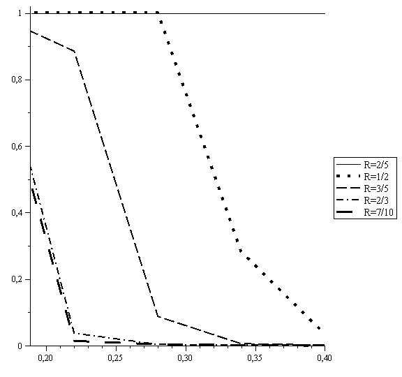
The new simulation for reverse-MDP convolutional codes shows that reverse-MDP codes only outperform MDS codes at low rates. If we compare Figures 2 and 3, one can see that only for rates equal to $R=2/5$ and $R=1/2$ the results are better using reverse-MDP convolutional codes.

However, observing the results in Figure 4, one can see how complete-MDP convolutional codes give much better performance than MDS block codes. Even though the rate decreases for convolutional codes when we increase the erasure probability, the behavior is better than in the MDS case.

For this reason we propose this kind of codes as a very good alternative to MDS block codes over this channel. Moreover, we believe that our proposed way of generating reverse-superregular matrices in Theorem 5.7, together with the construction for reverse-MDP convolutional codes given in Section 5, generates complete-MDP convolutional codes; so far we did not find any evidence of the opposite. Unfortunately, we were not able yet to prove this result; it remains an open question.

7 Comparison between MDS block codes and MDP convolutional codes

As we have already pointed out through several examples MDP convolutional codes often are capable of decoding more erasures than comparable MDS block codes. In this section we would like to give some theoretical results on the decoding capabilities of (complete) MDP convolutional codes and compare these codes with MDS block codes of the same rate.

As a first goal we will show that a rate $k/n$ convolutional code will not be able to decode erasures at a rate of more than $(n-k)/n$ . The following theorem serves this purpose.

Theorem 7.1.

Let $H(z)=\sum^{\nu}_{i=0}H_{i}z^{i}$ be the parity check matrix of an $(n,k,\delta)$ convolutional code. Assume $\text{$v$}(z)=\mathbf{v}_{0}+\mathbf{v}_{1}z+\ldots+\mathbf{v}_{l}z^{l}$ is a transmitted codeword and more than $(l+\nu+1)(n-k)$ erasures happen during transmission. Then unique decoding is not possible.

Proof:

$\text{$v$}(z)$ has to satisfy the linear system of equations as given in Equation $($ 2-B $)$ . The maximum number of erasures which uniquely can be decoded is hence given by the rank of the matrix appearing in Equation $($ 2-B $)$ . This rank is at most $(l+\nu+1)(n-k)$ . ∎

Corollary 7.2.

The maximum recovery rate of an $(n,k,\delta)$ convolutional code is at most $\frac{n-k}{n}$ .

Proof:

Theorem 7.1 shows that in a window of length $(l+1)n$ at most $(l+\nu+1)(n-k)$ erasures can be decoded. Taking the limit $l\longrightarrow\infty$ we see that not more than a ratio of $\frac{n-k}{n}$ erasures can be decoded. ∎

As a result we see that for long messages a rate $k/n$ convolutional code cannot decode at a rate larger than $(n-k)/n$ . On the other hand we have seen in Corollary 3.2 that an MDP convolutional code can decode all erasures as long as there are at most $(L+1)(n-k)$ in any sliding window of length $(L+1)n$ .

Compare this now with an $[N,K]$ linear block code $\mathcal{C}$ . The maximum number of erasures which can be decoded in any block of length $N$ is $N-K$ and this maximum is achieved by an MDS block code of rate $K/N$ . As a consequence the recovery rate of a rate $k/n$ MDP convolutional code and a rate $k/n$ block code are therefore the same ‘on average’. What matters for block codes is the block length and what matters for convolutional codes is the degree.

We conclude the section by comparing a $(2,1,\delta)$ convolutional code with an $[N,K]=[2\delta,\delta]$ block code.

Both these codes have rate $1/2$ . The $[2\delta,\delta]$ block code can decode all erasures as long as there are at most $\delta$ erasures in every slotted window (=block) of length $2\delta$ .

The performance of a $(2,1,\delta)$ (complete) MDP convolutional code is as follows:

By Corollary 3.2 unique decoding from left to right is possible as long as there are at most $(\delta+1)$ erasures in any sliding window of length $2\delta+2$ . If the $(2,1,\delta)$ code is also a complete MDP convolutional code then Theorem 6.6 states that decoding a whole window of length $6\delta+2$ can be achieved as long as there are not more than $2\delta+1$ erasures, and these erasures do not concentrate on the boundaries of the interval. In this way guard spaces can be computed and full decoding is possible via the forward, backward decoding process as we described it at length before.

The comparison shows that in order that a block code of rate $1/2$ can compete with a $(2,1,\delta)$ MDP convolutional code a block length of at least $2\delta$ is needed and even then there are many situations where full decoding is possible with the convolutional code and blocks of the linear block code cannot be decoded.

We conclude the section by comparing the decoding complexity.

An $[N,K]$ MDS block is capable of decoding $N-K$ erasures in every block. Assume $N-K$ erasures actually happen. If one works with the parity check matrix then the decoding task naturally translates into a linear system of the form $Ax=b$ , where $A$ is an $(N-K)\times(N-K)$ consisting of the columns of the parity check matrix where the erasures actually did happen. Alternatively one can work with the generator matrix of the code and again ends up with a linear system of the form $Ax=b$ , where $A$ is a $K\times K$ matrix consisting of the $K$ columns of the generator matrix where the transmission arrived correctly.

The number of field operations required to decode is hence of the order $O(r^{3})$ , where $r=\min\{K,N-K\}$ .

For an $(n,k,\delta)$ convolutional code the iterative decoding process as described in Theorem 3.1 requires again the solution of a linear system of the form $Ax=b$ , where $A$ is in the worst case of size $(L+1)(n-k)\times(L+1)(n-k)$ , in case one works with the parity check matrix $H(z)$ . If the number of erasures is relatively mild (always less than $(L+1)(n-k)$ erasures in any sliding window of length $(L+1)n$ ) then each system of equations of the form $Ax=b$ will decode one to several erasures at the time. If more erasures accumulate then Theorem 6.6 has to be invoked which requires the solution of a linear system $Ax=b$ of slightly larger size and this system possibly recovers just one erasure.

If $n(L+1)$ is comparable to the block length $N$ of the MDS block code then one sees that the computational effort is very comparable.

8 Conclusions

In this paper, we propose MDP convolutional codes as an alternative to MDS block codes when decoding over an erasure channel. MDP convolutional codes can be decoded iteratively ‘from left to right’ as long as the number of erasures in any sliding window does not surpass a certain amount (Corollary 3.2).

Reverse MDP convolutional codes are MDP convolutional codes having the extra property that erasures can also be decoded ‘from right to left’ as long as the number of erasures in any sliding window does not surpass a certain amount (Theorem 4.5).

Complete MDP convolutional codes are reverse MDP convolutional codes having the additional property that a whole interval can be decoded (independent of the past and the future) as long as the number of erasures does not surpass a certain amount (Theorem 6.6).

The maximum erasure recovery rate of a rate $k/n$ MDP convolutional code is $\frac{n-k}{n}$ . This is the same recovery rate as for a rate $k/n$ MDS block code often used in practice. In the case of an $[N,K]$ MDS block code error free decoding is possible if in every block at most $N-K$ erasures do happen. An $(n,k,\delta)$ MDP convolutional code can perform error free communication if in every sliding window of length $n(L+1)$ at most $(n-k)(L+1)$ errors do happen, where $L=\left\lfloor\frac{\delta}{k}\right\rfloor+\left\lfloor\frac{\delta}{n-k}\right\rfloor$ . When $N=nL$ then an MDS $[N,K]$ block code is comparable to an MDP convolutional code of the same rate. However simulation results show that even in this situation MDP convolutional codes perform better in case the convolutional code is a complete MDP convolutional code.

Acknowledgment

We would like to thank Martin Haenggi for explaining us the distribution of packet sizes when transmitting files over the Internet. The authors are also grateful to the anonymous referees for the many insightful comments they provided.

References

[1] M. Arai, A. Yamamoto, A. Yamaguchi, S. Fukumoto, and K. Iwasaki. Analysis of using convolutional codes to recover packet losses over burst erasure channels. In PRDC ’01: Proceedings of the 2001 Pacific Rim International Symposium on Dependable Computing, page 258, Washington, DC, USA, 2001. IEEE Computer Society.
[2] M. A. Epstein. Algebraic decoding for a binary erasure channel. Technical Report 340, Massachusetts Institute of Technology, March 1958. Reprinted from the 1958 IRE National Convention Record, Part 4.
[3] S. Fashandi, S.O. Gharan, and A.K. Khandani. Coding over an erasure channel with a large alphabet size. In Proc. of the IEEE International Symposium on Information Theory, (Toronto, Canada), pages 1053 –1057, July 2008.
[4] C. Fraleigh, S. Moon, B. Lyles, C. Cotton, M. Khan, D. Moll, R. Rockell, T. Seely, and C. Diot. Packet-level traffic measurements from the Sprint IP backbone. IEEE Network, 17:6–16, 2003.
[5] R.G. Gallager. Information Theory and Reliable Communication. John Wiley & Sons, New York, 1968.
[6] H. Gluesing-Luerssen, J. Rosenthal, and R. Smarandache. Strongly MDS convolutional codes. IEEE Trans. Inform. Theory, 52(2):584–598, 2006.
[7] H. Gluesing-Luerssen and F.-L. Tsang. A matrix ring description for cyclic convolutional codes. Adv. Math. Commun., 2(1):55–81, 2008.
[8] M. Hazewinkel. Moduli and canonical forms for linear dynamical systems III: The algebraic geometric case. In Proc. of the 76 Ames Research Center (NASA) Conference on Geometric Control Theory, pages 291–336. Math.Sci. Press, 1977.
[9] R. Hutchinson. The existence of strongly MDS convolutional codes. SIAM J. Control Optim., 47(6):2812–2826, 2008.
[10] R. Hutchinson, J. Rosenthal, and R. Smarandache. Convolutional codes with maximum distance profile. Systems & Control Letters, 54(1):53–63, 2005.
[11] R. Hutchinson, R. Smarandache, and J. Trumpf. On superregular matrices and MDP convolutional codes. Linear Algebra Appl., 428(11-12):2585–2596, 2008.
[12] R. Johannesson and K. Sh. Zigangirov. Fundamentals of Convolutional Coding. IEEE Press, New York, 1999.
[13] G. Kéri. Types of superregular matrices and the number of $n$ -arcs and complete $n$ -arcs in ${\rm PG}(r,q)$ . J. Combin. Des., 14(5):363–390, 2006.
[14] J. Lacan and J. Fimes. Systematic MDS erasure codes based on Vandermonde matrices. IEEE Communications Letters, 8(9):570–572, September 2004.
[15] S. Lee, Y. Won, and D.-J. Shin. On the multi-scale behavior of packet size distribution in internet backbone network. In 2008 IEEE Network Operations and Management Symposium, VOLS 1 AND 2, IEEE IFIP Network Operations and Management Symposium, pages 799–802, Salvador, Brazil, 2008.
[16] S. Lin and D. J. Costello Jr. Error Control Coding: Fundamentals and Applications. Prentice-Hall, Englewood Cliffs, NJ, 1983.
[17] M. Luby. LT codes. In Proceedings of the 43rd Symposium on Foundations of Computer Science, FOCS ’02, pages 271–, Washington, DC, USA, 2002. IEEE Computer Society.
[18] J. L. Massey. Reversible codes. Information and Control, 7(3):369–380, 1964.
[19] R. J. McEliece. The algebraic theory of convolutional codes. In V. Pless and W.C. Huffman, editors, Handbook of Coding Theory, volume 1, pages 1065–1138. Elsevier Science Publishers, Amsterdam, The Netherlands, 1998.
[20] M. Mushkin and I. Bar-David. Capacity and coding for the Gilbert-Elliott channels. IEEE Trans. Inform. Theory, 35(6):1277 – 1290, 1989.
[21] V. Paxson. End-to-end Internet packet dynamics. IEEE/ACM Trans. Netw., 7:277–292, June 1999.
[22] M. S. Ravi and J. Rosenthal. A smooth compactification of the space of transfer functions with fixed McMillan degree. Acta Appl. Math, 34:329–352, 1994.
[23] J. Rosenthal. Connections between linear systems and convolutional codes. In B. Marcus and J. Rosenthal, editors, Codes, Systems and Graphical Models, IMA Vol. 123, pages 39–66. Springer-Verlag, 2001.
[24] J. Rosenthal, J. M. Schumacher, and E. V. York. On behaviors and convolutional codes. IEEE Trans. Inform. Theory, 42(6, part 1):1881–1891, 1996.
[25] J. Rosenthal and R. Smarandache. Maximum distance separable convolutional codes. Appl. Algebra Engrg. Comm. Comput., 10(1):15–32, 1999.
[26] J. Rosenthal and E. V. York. BCH convolutional codes. IEEE Trans. Inform. Theory, 45(6):1833–1844, 1999.
[27] P. S. Rossi, G. Romano, F. Palmieri, and G. Iannello. Joint end-to-end loss-delay hidden Markov model for periodic UDP traffic over the Internet. IEEE Transactions on Signal Processing, 54(2):530–541, 2006.
[28] A. Shokrollahi. Raptor codes. IEEE Trans. Inform. Theory, 52(6):2551–2567, 2006.
[29] R. Sinha, C. Papadopoulos, and J. Heidemann. Internet packet size distributions: Some observations. Technical Report ISI-TR-2007-643, USC/Information Sciences Institute, May 2007.
[30] V. Tomás. Complete-MDP Convolutional Codes over the Erasure Channel. PhD thesis, Departamento de Ciencia de la Computacion e Inteligencia Artificial, Universidad de Alicante, Alicante, Spain, July 2010.
[31] V. Tomás, J. Rosenthal, and R. Smarandache. Decoding of MDP convolutional codes over the erasure channel. In Proceedings of the 2009 IEEE International Symposium on Information Theory, pages 556–560, Seoul, South Korea, 2009.
[32] V. Tomás, J. Rosenthal, and R. Smarandache. Reverse-maximum distance profile convolutional codes over the erasure channel. In Proceedings of the 19th International Symposium on Mathematical Theory of Networks and Systems – MTNS, pages 2121–2127, Budapest, Hungary, 2010.

Virtudes Tomás was born in Spain in 1983. She received her B.A. in Mathematics in 2006 from the University of Alicante with an Extraordinary Award. In 2010 she obtained the Ph.D. degree from the University of Alicante and her dissertation was supervised by Prof. Joan-Josep Climent and Prof. Joachim Rosenthal. Her thesis is in Coding Theory and its main topic is concerned with Complete-MDP convolutional codes. During her Ph.D. studies she was supported by an FPU Grant from the regional government of La Generalitat Valenciana (research grant for Ph.D. students) and enjoyed two research visits abroad, one in 2008 when she spent 12 months as a visitor at the University of Zürich (Zürich, Switzerland) and a second one in 2009 when she visited San Diego State University (San Diego, USA) for 2 months.

Joachim Rosenthal received the Diplom in Mathematics from the University of Basel in 1986 and the Ph.D. in Mathematics from Arizona State University in 1990. Since 2004 he has been Professor of Applied Mathematics at the University of Zürich where he currently also serves as Director of the Mathematics Institute. From 1990 until 2006 he has been with the University of Notre Dame, where he has last been the holder of an endowed chair in Applied Mathematics and also was Concurrent Professor in Electrical Engineering. In the academic year 1994/1995 he spent a sabbatical year at CWI the Center for Mathematics and Computer Science in Amsterdam, The Netherlands. During the academic year 1999/2000 he was a Guest Professor at the Swiss Federal Institute of Technology in Lausanne, Switzerland, affiliated with the School of Computer & Communication Sciences. His current research interests are in coding theory and cryptography. He currently serves as Associate Editor for Journal of Algebra and its Applications (JAA) and Advances in Mathematics of Communications (AMC). In the past he served also on the editorial boards of SIAM Journal on Control and Optimization (SICON), Mathematics of Control, Signals, and Systems (MCSS), Linear Algebra and its Applications (LAA) and Journal of Mathematical Systems, Estimation, and Control. In 2002 he served as the symposium chair of the International Symposium on Mathematical Theory of Networks and Systems (MTNS) and in 2010 he served together with M. Greferath as conference chair of the IEEE Information Theory Workshop in Dublin.

Roxana Smarandache is an associate professor in the Department of Mathematics and Statistics at San Diego State University. Originally from Bucharest, Romania, she has completed her undergraduate studies in mathematics at the University of Bucharest in 1996, with a B.S. thesis on Number Theory. From 1996-2001 she pursued a Ph.D. degree in Mathematics at the University of Notre Dame, which she completed in July 2001. Her thesis is in Coding Theory, with the subject of algebraic convolutional codes. After her Ph.D. she joined San Diego State University. During the academic year 1999-2000, Dr. Smarandache was for six months a visiting scholar at the Swiss Federal Institute of Technology (EPFL), Switzerland, in the Department of Communication Systems. During the academic year 2005-2006, she was on leave at the University of Notre Dame, on a visiting assistant professor position in the Department of Mathematics. During the academic year 2008-2009, she spent part of a sabbatical year at the University of Zurich (8 months) and part at the University of Notre Dame (3 months). Dr. Smarandache’s research topics are mainly related to coding theory. Her recent interests include low density parity check codes, iterative and linear programming decoding, and convolutional codes.

Decoding of Convolutional Codes over the Erasure Channel

Abstract

Index Terms:

1 Introduction

2 Preliminaries

2-A Erasure channel

2-B Convolutional codes

Lemma 2.1.

Proof:

Theorem 2.2.

Theorem 2.3.

3 Decoding over an erasure channel

Theorem 3.1.

Proof:

Corollary 3.2.

Proof:

Remark 3.3.

Remark 3.4.

Remark 3.5.

Example 3.6.

Remark 3.7.

4 The backward process and the reverse-MDP convolutional codes

Example 4.1.

Proposition 4.2.

Remark 4.3.

Definition 4.4.

Theorem 4.5.

Theorem 4.6.

Remark 4.7.

Proof:

Remark 4.8.

Example 4.9.

Remark 4.10.

5 Construction of reverse-MDP Convolutional Codes

Definition 5.1.

Remark 5.2.

Definition 5.3.

Example 5.4.

Example 5.5.

Example 5.6.

5-A Construction of reverse-superregular matrices

Theorem 5.7.

Proof:

Theorem 5.8.

Proof:

Theorem 5.9.

Proof:

Theorem 5.10.

Proof:

Example 5.11.

Theorem 5.12.

Example 5.13.

Example 5.14.

Theorem 5.15.

Example 5.16.

6 Complete-MDP convolutional codes

Definition 6.1.

Remark 6.2.

Example 6.3.

Lemma 6.4.

Proof:

Example 6.5.

Theorem 6.6.

Proof:

Example 6.7.

6-A Simulations

7 Comparison between MDS block codes and MDP convolutional codes

Theorem 7.1.

Proof:

Corollary 7.2.

Proof:

8 Conclusions

Acknowledgment

References

Decoding of Convolutional Codes
over the Erasure Channel