Beer-Sheva, 84105, Israel. dolev@cs.bgu.ac.il55footnotetext: INRIA REGAL, France.66footnotetext: Laboratoire IBISC-EA 4526, 91000 Evry, France. stephane.rovedakis@ibisc.fr
Fast Self-Stabilizing Minimum Spanning Tree Construction
Using Compact Nearest Common Ancestor Labeling Scheme
Abstract
We present a novel self-stabilizing algorithm for minimum spanning tree (MST) construction. The space complexity of our solution is bits and it converges in rounds. Thus, this algorithm improves the convergence time of all previously known self-stabilizing asynchronous MST algorithms by a multiplicative factor , to the price of increasing the best known space complexity by a factor . The main ingredient used in our algorithm is the design, for the first time in self-stabilizing settings, of a labeling scheme for computing the nearest common ancestor with only bits.
1 Introduction
Since its introduction in a centralized context [15, 14], the minimum spanning tree (or MST) problem gained a benchmark status in distributed computing thanks to the seminal work of Gallager, Humblet and Spira [9].
The emergence of large scale and dynamic systems, often subject to transient faults, revives the study of scalable and self-stabilizing algorithms. A scalable algorithm does not rely on any global parameter of the system (e.g. upper bound on the number of nodes or the diameter). Self-stabilization introduced first by Dijkstra in [6] and later publicized by several books [7, 8] deals with the ability of a system to recover from catastrophic situation (i.e., the global state may be arbitrarily far from a legal state) without external (e.g. human) intervention in finite time.
Although there already exists self-stabilizing solutions for the MST construction, none of them considered the extension of the Gallager, Humblet and Spira algorithm (GHS) to self-stabilizing settings. Interestingly, this algorithm unifies the best properties for designing large scale MSTs: it is fast and totally decentralized and it does not rely on any global parameter of the system. Our work proposes an extension of this algorithm to self-stabilizing settings. Our extension uses only logarithmic memory and preserves all the good characteristics of the original solution in terms of convergence time and scalability.
Gupta and Srimani presented in [13] the first self-stabilizing algorithm for the MST problem. The MST construction is based on the computation of all shortest paths (for a certain cost function) between all pairs of nodes. While executing the algorithm, every node stores the cost of all paths from it to all the other nodes. To implement this algorithm, the authors assume that every node knows the number of nodes in the network, and that the identifiers of the nodes are in . Every node stores the weight of the edge placed in the MST for each node . Therefore the algorithm requires bits of memory at node . Since all the weights are distinct integers, the memory requirement at each node is bits. The main drawback of this solution is its lack of scalability since each node has to know and maintain information for all the nodes in the system. Note also that the time complexity announced by the authors, stays only in the particular synchronous settings considered by the authors. In asynchronous setting the complexity is rounds. A different approach for the message-passing model, was proposed by Higham and Liang [11]. The algorithm performs roughly as follows: every edge checks whether it eventually belongs to the MST or not. To this end, every non tree-edge floods the network to find a potential cycle, and when receives its own message back along a cycle, it uses the information collected by this message (i.e., the maximum edge weight of the traversed cycle) to decide whether could potentially be in the MST or not. If the edge has not received its message back after the time-out interval, it decides to become tree edge. The memory used by each node is bits, but the information exchanged between neighboring nodes is of size bits, thus only slightly improving that of [13]. This solution also assume that each node has access to a global parameter of the system: the diameter. Its computation is expensive in large scale systems and becomes even harder in dynamic settings. The time complexity of this approach is rounds where and are the number of edges and the diameter of the network respectively, i.e., rounds in the worst case.
In [2] we proposed a self-stabilizing loop-free algorithm for the MST problem. Contrary to previous self-stabilizing MST protocols, this algorithm does not make any assumption on the network size (including upper bounds) or the unicity of the edge weights. The proposed solution improves on the memory space usage since each participant needs only bits while preserving the same time complexity as the algorithm in [11].
Clearly, in the self-stabilizing implementation of the MST algorithms there is a trade-off between
the memory complexity and their time complexity (see Table 1, where a boldface denotes the most useful (or efficient) feature for a particular criterium). The challenge we address in this paper is to design fast
and scalable self-stabilizing MST with little memory. Our approach brings together two worlds: the time efficient
MST constructions and the memory compact informative labeling schemes.
Therefore, we extend
the GHS algorithm to self-stabilizing settings and keep compact its
memory space by using a self-stabilizing extension
of the nearest common ancestor labeling scheme of [1].
Note that labeling schemes have already been used in
order to infer a broad set of information such as
vertex adjacency, distance, tree ancestry or tree routing [5],
however none of these schemes have been studied in self-stabilizing
settings (except the last one).
Our contribution is therefore twofold. We propose for the first time in self-stabilizing settings a bits scheme for computing the nearest common ancestor. Furthermore, based on this scheme, we describe a new self-stabilizing algorithm for the MST problem. Our algorithm does not make any assumption on the network size (including upper bounds) or the existence of an a priori known root. Moreover, our solution is the best space/time compromise over the existing self-stabilizing MST solutions. The convergence time is asynchronous rounds and the memory space per node is bits. Interestingly, our work is the first to prove the effectiveness of an informative labeling scheme in self-stabilizing settings and therefore opens a wide research path in this direction.
2 Model and notations
We consider an undirected weighted connected network where is the set of nodes, is the set of edges and is a positive cost function. Nodes represent processors and edges represent bidirectional communication links. Additionally, we consider that is a network in which the weight of the communication links may change value.
The processors asynchronously execute their programs consisting of a set of variables and a finite set of rules. The variables are part of the shared register which is used to communicate with the neighbors. A processor can read and write its own registers and can read the shared registers of its neighbors. Each processor executes a program consisting of a sequence of guarded rules. Each rule contains a guard (Boolean expression over the variables of a node and its neighborhood) and an action (update of the node variables only). Any rule whose guard is true is said to be enabled. A node with one or more enabled rules is said to be privileged and may make a move executing the action corresponding to the chosen enabled rule.
A local state of a node is the value of the local variables of the node and the state of its program counter. A configuration of the system is the cross product of the local states of all nodes in the system. The transition from a configuration to the next one is produced by the execution of an action at a node. A computation of the system is defined as a weakly fair, maximal sequence of configurations, , where each configuration follows from by the execution of a single action of at least one node. During an execution step, one or more processors execute an action and a processor may take at most one action. Weak fairness of the sequence means that if any action in is continuously enabled along the sequence, it is eventually chosen for execution. Maximality means that the sequence is either infinite, or it is finite and no action of is enabled in the final global state.
In the sequel we consider the system can start in any configuration. That is, the local state of a node can be corrupted. Note that we don’t make any assumption on the bound of corrupted nodes. In the worst case all the nodes in the system may start in a corrupted configuration. In order to tackle these faults we use self-stabilization techniques.
Definition 1 (self-stabilization)
Let be a non-empty legitimacy predicate11
1
A legitimacy predicate is defined over the configurations of a system and is an indicator of its correct behavior. of an algorithm with respect to a specification predicate such that every configuration satisfying satisfies . Algorithm is self-stabilizing with respect to iff the following two conditions hold:
(i) Every computation of starting from a configuration satisfying preserves (closure).
(ii) Every computation of starting from an arbitrary configuration contains a configuration that satisfies (convergence).
3 Overview of our solution
We propose to extend the Gallager, Humblet and Spira (GHS) algorithm, [9], to self-stabilizing settings via a compact informative labeling scheme. Thus, the resulting solution presents several advantages appealing for large scale systems: it is compact since it uses only logarithmic memory in the size of the network, it scales well since it does not rely on any global parameter of the system, it is fast — its time complexity is the better known in self-stabilizing settings. Additionally, it self-recovers from any transient fault.
The central notion in the GHS approach is the notion of fragment. A fragment is a partial spanning tree of the graph, i.e., a fragment is a tree which spans a subset of nodes. Note that a fragment can be limited to a single node. An outgoing edge of a fragment is an edge with a unique endpoint in . The minimum-weight outgoing edge of a fragment is denoted in the following as MEF. In the GHS construction, initially each node is a fragment. For each fragment , the GHS algorithm in [9] identifies the MEF and merges the two fragments endpoints of MEF. Note that, with this scheme, more than two fragments may be merged concurrently. The merging process is recursively repeated until a single fragment remains. The result is a MST. The above approach is often called “blue rule” for MST construction.
This approach is particularly appealing when transient faults yield to a forest of fragments (which are sub-trees of a MST). The direct application of the blue rule allows the system to reconstruct a MST and to recover from faults which have divided the existing MST. However, when more severe faults hit the system the process variables may be corrupted leading to a configuration of the network where the set of fragments are not sub-trees of some MST. That is, it may be a spanning tree but not of minimum weight, or it can contain cycles. In this case, the application of the blue rule only is not sufficient to reconstruct a MST. To overcome this difficulty, we combine the blue rule with another method, referred in the literature as the “red rule”. The red rule removes the heaviest edge from every cycle. The resulting configuration contains a MST. We use the red rule as follows: given a spanning tree of , every edge of that is not in is added to , thus creating a (unique) cycle in . This cycle is called a fundamental cycle, denoted by . If is not the edge of maximum weight in , then, according to the red rule, there exists an edge in with . The edge of maximum weight can be removed since it is not part of any MST.
Our MST construction combines both the blue and red rules. The blue rule application needs that each node identifies its own fragment. The red rule requires that nodes identify the fundamental cycle corresponding to every adjacent non-tree-edge. In both cases, we use a self-stabilizing labeling scheme, called NCA-L, which provides at each node a distinct informative label such that the nearest common ancestor of two nodes can be identified based only on the labels of these nodes (see Section 3.1). Thus, the advantage of this labeling is twofold. First the labeling helps nodes to identify their fragments. Second, given any non-tree edge , the path in the tree going from to the nearest common ancestor of and , then from there to , and finally back to by traversing , constitute the fundamental cycle .
To summarize, our algorithm will use the blue rule to construct a spanning tree, and the red rule to recover from invalid configurations. In both cases, it uses our algorithm NCA-L to identify both fragments and fundamental cycles. Note that, in [3, 4] distributed algorithms using the blue and red rules to construct a MST in a dynamic network are proposed, however these algorithms are not self-stabilizing.
Variables used by NCA-L and MST modules
For any node , we denote by the set of all neighbors of in . We use the following notations:
- •
: the parent of in the current spanning tree, an integer pointer to a neighbor;
- •
: the label of composed of a list of pairs of integers where each pair is an identifier and a distance (the size of is bounded by bits);
- •
: a pair of variables, the first one is an integer the number of nodes in the sub-tree rooted at and the second one is the identifier of the child of with the maximum number of nodes in the sub-tree rooted at ;
- •
: the minimum weighted edge composed by a pair of variables, the first one is an integer, the weight of the edge and the second one is the label of a node stored in .
3.1 Self-stabilizing Nearest Common Ancestor Labeling
Our labeling scheme, called in the following NCA-L, uses the notions of heavy and light edges introduced in [10]. In a tree, a heavy edge is an edge between a node and one of its children of maximum number of nodes in its sub-tree. The other edges between and its other children are tagged as light edges. We extend this edge designation to the nodes, a node is called heavy node if the edge between and its parent is a heavy edge, otherwise is called light node. Moreover, the root of a tree is a heavy node. The idea of the scheme is as follows. A tree is recursively divided into disjoint paths: the heavy and the light paths which contain only heavy and light edges respectively.
-
-
-
-
-
-
-
-
-
-
-
To label the nodes in a tree , the size of each subtree rooted at each node of is needed to identify heavy edges leading the heaviest subtrees at each level of . To this end, each node maintains a variable named which is a pair of integers. The first integer is the local estimation of the number of nodes in the subtree rooted at . The second integer is the identifier of a child of with maximum number of nodes. That is, it indicates the heavy edge. The computation of is processed from the leaves to the root (see Predicate in Figure 1). A leaf has no child, therefore for a leaf node (see Predicate in Figure 1 and Rule Rℓ).
Based on the heavy and light nodes in a tree indicated by variable at each node , each node of can compute its label. The label of a node stored in is a list of pair of integers. Each pair of the list contains the identifier of a node and a distance to the root of the heavy path (i.e., a path including only heavy edges). For the root of a fragment, the label is the following pair , respectively the identifier of and the distance to itself, i.e., zero (see Rule R⊙). When a node is tagged by its parent as a heavy node (i.e., ), then the node takes the label of its parent but it increases by one the distance of the last pair of the parent label. Examples of theses cases are given in Figure 2, where integers inside the nodes are node identifiers and lists of pairs of values are node labels. When a node is tagged by its parent as a light node (i.e., ), then the node becomes the root of a heavy path and it takes the label of its parent to which it adds a pair of integers composed of its identifier and a zero distance (see Figure 2).
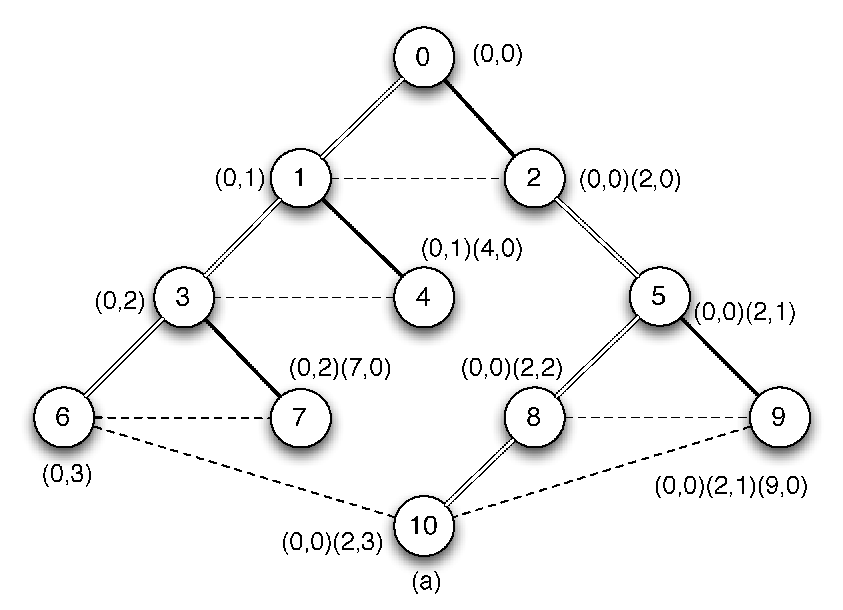
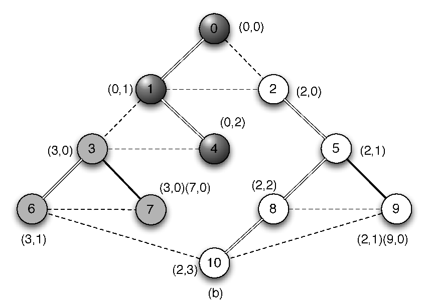

This labeling scheme is used in second part of this article in MST algorithm to find the minimum weighted edges, but it is also used to detect and destroy cycles since the initial configuration may not be a spanning tree. To this end, we define an order on the
labels of nodes.
Let and be two nodes and
and be their respective labels
such that and
with . The label of a node is lower than the label of node , noted , if (1) and , or (2) or (3) and .
A node can detect the presence of a cycle by only comparing its label with the label of its parent. That is, if its label is contained in the label of its parent, or it is inferior to the one of its parent then is part of a cycle (see Predicate in Figure 1). In this case, the node becomes the root of its fragment in order to break the cycle (see below Rule R⊙).
Algorithm NCA-L is composed of two rules. Rule R⊙ creates a root or breaks cycles while rule Rℓ produces a proper labeling. Note that the last predicates in rules R⊙ and Rℓ (the part in gray) are used only for insuring the exclusivity of rules execution when the labeling scheme works together with the MST scheme.
A node with an incoherent parent (which is not one of its neighbors)
or present in a cycle executes R⊙. Following the execution of this rule
node becomes a root node, it sets its parent to void and its label to .
Rule Rℓ helps a node to compute the number of nodes in its sub-tree (stored in variable ) and provides to a coherent label.
- R⊙: [ Root creation
-
]
If
Then ;
- Rℓ: [ Label correction
-
]
If
Then If then
Else
If
Else
3.2 Self-stabilizing MST
In this section we describe our self-stabilizing MST algorithm. The algorithm executes two phases: the MST correction and the MST fragments merging. Recall that our algorithm uses the blue rule to construct a spanning tree and the red rule to recover from invalid configurations. In both cases, it uses the nearest-common ancestor labeling scheme to identify fragments and fundamental cycles. We assume in the following that the merging operations have a higher priority than the recovering operations. That is, the system recovers from an invalid configuration if and only if no merging operation is possible. In the worst case, after a failure hit the system, a merging phase will be followed by a recovering phase and finally by a final merging phase.
3.2.1 The minimum weighted edge and MST correction
-
-
-
-
-
-
-
-
-
-
-
-
-
Note that the scope of our labeling scheme is twofold. First, it allows a node to identify the neighbors that share the same fragment and consequently to select the outgoing edges of a fragment. Second, the labeling scheme may be used to identify cycles and to repair the tree. To this end, the algorithm uses the nearest common ancestor predicate depicted in Figure 1. For two nodes and with a non tree edge (i.e., and ), if the nearest common ancestor does not exist then and are in two distinct fragments (i.e., if we have ). Otherwise and are in the same fragment and the addition of to generates a cycle. Let be the set of edges on the unique path between and in , with . The fundamental cycle is the following: . Consider the example depicted on Figure 2(b). The labels of nodes and are respectively and . In this case so the edge is an outgoing edge because the nodes and are in two distinct fragments and they have no common ancestor. If the edge is of minimum weight then can be used for a merging between the fragment rooted in and the fragment rooted in . For the case of nodes and the labels are and and . Consequently, and are in the same fragment. The fundamental cycle with goes through the node with the label , in other word the node in Figure 2(b).
Predicate (see Figure 3) computes both the minimum weight outgoing edge used in a merging phase and the internal edges used in a recovering phase. Our algorithm gives priority to the computation of minimum outgoing edges via Predicate . A recovering phase is initiated if there exists a unique tree or if a sub-tree of one fragment has no outgoing edge.
The computation of the minimum weight outgoing edge is done in a fragment if and only an adjacent fragment is detected by , i.e., if we have Predicate . In this case, using Rule RMin each node collects from the leaves to the root the outgoing edges leading to an adjacent fragment . At each level in a fragment, a node selects the outgoing edge of minimum weight among the outgoing edges selected by its children and its adjacent outgoing edges. Thus, this allows to the root of a fragment to select the minimum outgoing edge of the fragment leading to an adjacent fragment. Then, the edge can be used to perform a merging between two adjacent fragments using an edge belonging to a MST.
Let us explain Rule R↯ which allows to correct a tree (or a fragment). In this case, the information about the non-tree edges are sent to the root as follows. Among all its non-tree edges, a node sends the edge with the nearest to the root (see Figure 4(a)). The information about the edge is stored in variable . If the parent of the node has the same information and the weight of the edge then the edge is removed from the tree (see Figure 4(a-b) for the nodes 6 and 10). We use the red rule in an intensive way, because we remove all the edges with a weight upper than in fundamental cycle of . This interpretation of the red rule allows to insure that after a recovering phase the remaining edges belong to a MST.
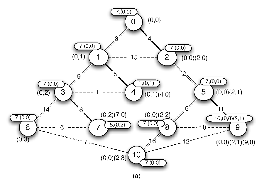
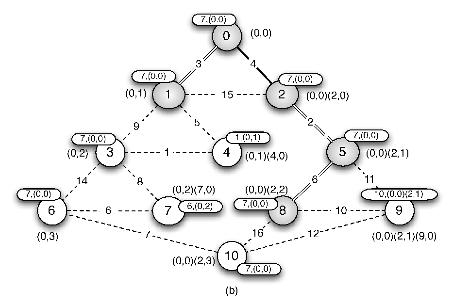
-
RMin: [ Minimum computation ]
If
Then
-
R↯: [ MST Correction ]
If
Then
To summarize, in this section we explained how to compute the outgoing-edges and the fundamental cycles (Rule RMin), and how to recover from a false tree (Rule R↯). The next section addresses the fragments merging operation (Rules R⊳⊲ and R⎔).
3.2.2 Fragments merging
In this phase two rules are executed: R⊳⊲ and R⎔. Note that Rule RMin (described in the previous section) computes from the leaves to the root the minimum outgoing edge of the fragment , with . The information about are stored in the variable mwe, i.e., the weight of the edge and a common ancestor equal to to indicate that these information concern an outgoing edge. When a root of has stabilized its variable , it starts a merging phase (Rule R⊳⊲). To this end, the nodes in the path between and are reoriented from to . During this reorientation the labels are locked. That is, each node on the path between and (including and excluding ) changes its label to: . When a node becomes the root of the fragment it can merge with the fragment . After the addition of the outgoing edge , the labeling process is re-started (see Rule R⎔). The merging phase is repeated until a single fragment is obtained.
-
R⊳⊲: [ Merging ]
If
Then
If
Then
;
If
Then ;
Else
;
-
R⎔: [ End Merging ]
If
Then ;
4 Correctness proof
Lemma 1
Let a configuration where the set of variables form at least one cycle in the network. In a finite time, Algorithm NCA-L removes all the cycles from the network.
Proof. If a node has a parent which is not in its neighborhood or if has no parent then the parent and the label variable of is modified to and respectively with Rule R⊙.
A node identifies a cycle with Predicate which uses ’s label and the label of its parent. In a legitimate configuration, ’s label is smaller than the label of its parent and is constructed using the label of its parent, i.e., the label of the parent of is included to ’s label. Thus, if the label of is included or is smaller than the label of its parent then a cycle is detected and Predicate is true. In this case, reinitiates its parent and label variable using Rule R⊙.
In order to detect a cycle the label computation process must cross a part or all the nodes of the cycle. However, since we consider a distributed scheduler then all the nodes in a cycle can be activated and we can have a rotation of the labels of the nodes in the cycle. This may lead to a new configuration in which the labels cannot be used to detect a cycle, because the label of one node is not used to compute some other labels and to detect a cycle. To break this symmetry, we use the node identifiers with Predicate . This predicate allows to activate the node iff has no neighbor such that is activated and ’s identifier is lower than . Therefore, there is at least a node in the cycle which is not activated and when the label of is used by some other nodes to compute their labels then Predicate is true and breaks the cycle using Rule R⊙.
According to Lemma 1, if the system starts from a configuration which contains at least one cycle then all the cycles are removed from the network in a finite time. Therefore, in the following we consider only configurations containing no cycle.
Definition 2 (Legitimate state of NCA-L)
Let a configuration with no cycle in the network, i.e., which contains a forest of trees . The configuration is legitimate for Algorithm NCA-L iff each node satisfies one of the following conditions:
- 1.
the label of is equal to , if the edge between and ’s parent in is a light edge or is the root of the tree;
- 2.
the label of is equal to and , if the edge between and ’s parent in is a heavy edge.
Lemma 2 (Convergence for NCA-L)
Starting from an illegitimate configuration for Algorithm NCA-L, eventually Algorithm NCA-L reaches in a finite time a legitimate configuration.
Proof. To compute correct node labels, heavy and light edges in each tree of the forest in the network must be identified. To this end, each node maintains in the variable two information: the size of its subtree in and the identifier of the child with the subtree of maximum number of nodes. Based on the first information given by its children stored in variable , each node compute the size of its subtree in and informs its child if the edge is a light or heavy edge. The edge is a heavy edge if the second information stored in is equal to the identifier of , a light edge otherwise. Therefore, each node can detect if its label is correct according to its parent label. Note that Predicate is used at node to help to break cycle if we are in the case of a configuration described in proof of Lemma 1. Moreover, since we use the labeling scheme with minimum spanning tree computation rules Predicate is used to forbid the label correction when it has been modified by Rule and R⎔.
The computation of the information stored in the variable at each node is done via bottom-up fashion in the tree . According to Predicate , if the variable is not equal to at a leaf node in then Predicate and can execute Rule Rℓ to correct its variable . Otherwise according to Predicate , for any internal node the first information of must be equal to one plus the sum of the size of the children subtrees and the second one to the identifier of its child with the maximum subtree size. Thus, if variable is not correct (i.e., Predicate ) then can execute Rule Rℓ to correct its variable . Using the same argument, one can show by induction that for any internal node we have .
The computation of the node labels in a tree is done via top-down fashion starting from the root of . For convenience, a path is called heavy (resp. light) if it contains only heavy (resp. light) edges. Moreover, a node is called heavy (resp. light) if the edge between its parent and itself is a heavy (resp. light) edge. is informed by its parent with if is a heavy (i.e., ) or light (i.e., ) node. The root node of is also the root of a heavy path and its label must be equal to . According to Predicate and , can execute Rule Rℓ to correct its label. Otherwise, we have two cases: heavy or light nodes. When the root have a correct label then all its children can compute their correct label. If a heavy (resp. light) node has a label different from and (resp. ) then we have Predicate (resp. ), and . Therefore, can execute Rule Rℓ to correct its label accordingly with its parent. Using the same argument, one can show by induction that for any internal node we have and (resp. ) for heavy (resp. light) nodes.
Lemma 3 (Closure for NCA-L)
The set of legitimate configurations for NCA-L is closed.
Proof. According to Algorithm NCA-L, the labeling procedure is done using only Rule Rℓ. In any legitimate configuration for Algorithm NCA-L, for any node Predicate and are true and Rule Rℓ cannot be executed by a node . So, starting from a legitimate configuration for Algorithm NCA-L the system remains in a legitimate configuration.
Definition 3 (Legitimate state of MST)
A configuration is legitimate for Algorithm MST iff each node satisfies the following conditions:
- 1.
a tree spanning the set of nodes in is constructed;
- 2.
is of minimum weight among all spanning trees.
Lemma 4
Let a tree (or fragment). Eventually for each node the variable contains a pair of values: the weight of the minimum outgoing edge of the fragment and , if a merging is possible between two fragments and , .
Proof. We assume that and , are two distinct coherent trees (i.e., different root and correct labels, otherwise Rule R⊙ and Rℓ are used to correct the trees) in the network and that a merging is possible between and . The computation of the minimum outgoing edge of (resp. ) is done in a bottom-up fashion. We consider the tree but the computation in is done in a same way. A leaf node can compute and store in its variable its local adjacent minimum outgoing edge leading to another tree. Macro returns the local minimum outgoing edge if Macro . To this end, if there is an adjacent outgoing edge leading to another tree (i.e., and ) and we have then can execute Rule RMin to compute its local outgoing edge stored in the variable . A internal node must use the local outgoing edges computed by its children and selects the edge of minimum weight among these edges, then it compares this value with the weight of its adjacent local outgoing edge and again it holds the edge of minimum weight. The selection of its children minimum outgoing edge is done by Macro and the computation of its local outgoing edge is done by Macro as for a leaf node. Thus, if there is an outgoing edge which can be used to make a merging with another tree (i.e., ) and we have for a internal node , then can execute Rule RMin to compute in the variable its local minimum outgoing edge. Using the same argument, one can show by induction that for any internal node we have . Therefore, the local outgoing edge computed by the root node is the minimum outgoing edge of .
Lemma 5
Let a tree (or fragment). Eventually for each node the variable contains a pair of values: the weight of an edge and the label of the nearest common ancestor of and . Moreover, eventually all local internal edges of are computed.
Proof. We assume that is a coherent tree, otherwise Rule R⊙ and Rℓ are used to break the cycles and to correct the labels. Each node starts to compute local internal edges (i.e., edges such that and or or is in the subtree of ) when it has no local outgoing edge (adjacent outgoing edge or outgoing edge given by a child) leading to another tree. In this case, a node informs its parent of its local internal edges using its variable . Macro returns the local internal edge of which has the common ancestor nearest from the root among the internal edges that were not taken into account by its parent using the node labels. Each node which is in a recover phase sends all its local internal edges. To this end, compute its next local internal edge when its parent has taken into account ’s current local internal edge (i.e., ). Thus, the information of internal edges are put back up in the tree until reaching the nearest common ancestor and do not wait an acknowledgement from the nearest common ancestor to send its next internal edge. Moreover, Macro compute the next internal edge adjacent to such that the label of the nearest common ancestor associated to with is greater (according to operator ) than which is used to define an order on the internal edges. Otherwise, if then according to Macro the node reset the computation of its adjacent internal edge to assure that every internal edge is taken into account. The recover phase is started at node if has no local outgoing edge (i.e., ) and ’s parent has taken into account the information associated to its current internal edge and stored in variable (i.e., ). In this case, the guard of Rule RMin is satisfied and can execute Rule RMin to update its variable with the information of its next local internal edge. The information given by a child are stopped at the nearest common ancestor of the corresponding internal edge since Macro selects only from a child such that .
Lemma 6
Let a tree and any edge . Eventually, if is not part of a minimum spanning tree of the network then is removed from .
Proof. We assume that is a coherent tree, otherwise Rule R⊙ and Rℓ are used to break the cycles and to correct node labels. Let an edge (w.l.o.g. ) which is not part of a minimum spanning tree. As the network has a finite size then there is a time after which there exists no merging between two trees in the network. Thus according to Lemma 5 each internal edge of is put back up in until reaching the nearest common ancestor associated to . Since is not in a minimum spanning tree, there is an edge such that and is on the path between and or between and . So, there is a time such that and according to Lemma 5. Then Predicate returns true because we have and . Therefore, can execute Rule R↯ to create a new tree rooted at and as a consequence the edge is removed from .
Lemma 7
Let two distinct trees and with . Let an edge such that is part of a minimum spanning tree and and . Eventually is used to merge the trees and .
Proof. We assume that and are coherent trees, otherwise Rule R⊙ and Rℓ are used to break the cycles and to correct node labels. According to Lemma 4, the merging edge is computed by the root and it starts the merging phase since only the root can choose the edge of minimum weight leading to another tree to use in order to make a merging. In the remainder, we focus on tree but the same arguments are also true for .
When the root has finished to compute its minimum outgoing edge from its fragment (i.e., we have ) then can execute Rule R⊳⊲ because Predicate is satisfied since has a coherent label. Note that we permit the creation of cycles of length two only if at least one node has a label equal to . Indeed, during the merging phase the orientation is reversed on the path between the root of and the node adjacent to the edge used for the merging, that is why a cycle is detected in Rule R⊙ if Predicate is not satisfied. Thus, can change its variables and as following. If there is an edge adjacent to such that and then selects as its new parent (only if ) and changes its label to to informs its subtree that the merging is done. Otherwise, selects its child such that as its new parent and changes its label to to inform that a merging is started.
Any other node on the path between the root and the node adjacent to the merging edge take part in the merging phase when its parent has selected as its new parent (i.e., ) and ’s parent label is equal to . Thus, Predicate is satisfied and can execute Rule R⊳⊲ since (otherwise Rule RMin is executed to update its variable ). So, changes its variables and as described above for the root. Since the merging phase is done on a path, using the same argument one can show by induction that for any internal node on the path between the root and the node adjacent to the merging edge (except for ) we have and and for the node we have and .
Lemma 8
Eventually all the nodes have a correct label in the new fragment resulting from a merging phase.
Proof. According to Lemma 7, a merging phase is done using the minimum outgoing edge between two distinct trees and if it is possible. Moreover, when the edge is added by the extremity of minimum identifier, w.l.o.g. let , then ’s label is equal to and the end of the merging phase is propagated in the resulting fragment . In the reminder we focus on tree but the same arguments are true for tree .
Let the node such that and (i.e., is the child of on the path between and the old root of ). Predicate is false because is not a root node and the label of its parent is not equal to . Moreover, Predicate is true since ’s label is equal to and ’s label to . Thus, can execute Rule R⎔ to modify its label to . Using the same argument, one can show by induction that every node on the path between and the old root of can execute Rule R⎔, thus there is a time such that we have .
Now we show that the other nodes in can execute Rule R⎔. Consider the node such that is the old root of and . Let a node such that . Predicate is false because is not a root node and the label of its parent is not equal to . Moreover, Predicate is true because and ’s label is not equal to since is not on the path between and the old root of , and ’s label is different from . Note that since the start of the merging phase, Predicate is true because Predicate or is true. So, Rule Rℓ cannot be executed by and ’s label has not changed. Thus, can execute Rule R⎔ to modify its label to . Using the same argument, one can show by induction that every node on the path between and a leaf node can execute Rule R⎔, thus there is a time such that we have .
Every node in the resulting fragment can execute Rule Rℓ when the edge is added in and ’s label has been modified from to its new label based on ’s label. Indeed, in this case for every node , with and , Predicate is false and can execute Rule Rℓ. Therefore, there is a time such that every node in has a correct label.
Lemma 9 (Convergence for MST)
Starting from an illegitimate configuration for Algorithm MST, eventually Algorithm MST reaches in a finite time a legitimate configuration.
Proof. We assume that there is a forest of trees , in the network, otherwise according to Lemma 1 Rule R⊙ is executed to remove the cycle from the network. Moreover, we assume also that the node’s label are correct in tree , otherwise according to Lemma 2 and 3 there is a time such that the node’s label are corrected.
According to Lemma 5 and 6, if an edge and is part of no minimum spanning tree of the network then is removed from tree . Thus, there is a time such that the existing fragments in the network are part of a minimum spanning tree. According to Lemmas 4 and 7, eventually if there are at least two distinct fragments then a merging phase is started. Moreover, node labels are corrected after a merging phase according to Lemma 8. Since the size of the network is finite there is a finite number of merging. Therefore, in a finite time a spanning tree of minimum weight is computed by Algorithm MST.
Lemma 10 (Closure for MST)
The set of legitimate configurations for MST is closed.
Proof. Let a legitimate configuration such is a minimum spanning tree of the network and an edge . To be illegitimate, the configuration must contain an edge such that it exists an edge with and and are included in the same fundamental cycle . Thus, this imply that the edge is not used to verify if it is possible to replace an edge of with which contradicts Lemmas 5 and 6. Moreover, since is a spanning tree then no merging is done in the network. Therefore, starting from a legitimate configuration for Algorithm MST a legitimate configuration is preserved.
5 Complexity proofs
In the following we discuss the complexity issues of our solution.
Lemma 11
Algorithms NCA-L and MST have a space complexity of bits.
Proof. Algorithm NCA-L uses three variables : . The first and the last one are respectively a pointer to a neighbor node and a pair of integers, each one needs bits. However, the variable is a list of pairs of integers. A new pair of integers is added to the list when a light edge is created in the tree. As noticed in [1], there are at most light edges on the path from a leaf to the root, i.e., at most pairs of integers. Thus, the variable uses bits.
Algorithm MST uses an additional variable which is a pair composed of an integer and the label of a node. The label of a node is stored in variable which uses bits. Thus, the variable needs bits.
Therefore, Algorithms NCA-L and MST use bits of memory at each node.
Lemma 12
Starting from any configuration, all cycles are removed from the network in at most rounds, with the number of nodes in the network.
Proof. As explained in the proof of Lemma 1, to break a cycle a part of the nodes in must compute their new labels, that is a label computation must be initiated from one node and then this process must cross . Thus, the worst case is a configuration in which all the nodes in have to compute their new labels using Rule Rℓ to detect the presence of cycle . Therefore, at most rounds are needed to compute the new label of the nodes in based on the label of one node in . According to Lemma 1, when this computation is done the cycle is detected and removed by the node . At most additional rounds are needed to break the cycle .
Since there is at most cycles in a network, at most rounds are needed to remove all the cycles from the network.
Lemma 13
Starting from a configuration which contains a tree , using Algorithm NCA-L any node has a correct label in at most rounds.
Proof. As described in proof of Lemma 2, the correction of node labels is done using a bottom-up computation followed by a top-down computation in the tree .
The bottom-up computation is started by the leaves of , when leaf nodes have corrected their variable to then internal nodes can start to correct their variable . An internal node computes a correct value in its variable using Rule Rℓ when all its children have a correct value in their variable . Since the computation is done in a tree sub-graph then in at most rounds each node has corrected its variable .
The top-down computation is started by the root of the tree . When the root has a correct value in variable then the computation of correct labels can start. Thus, if the parent of a node has a correct value in its variable and then can compute its correct label in using Rule Rℓ. As for the bottom-up computation, the top-down computation is done in at most rounds since it is performed in a tree sub-graph.
Therefore, in at most rounds each node in the tree has a correct label stored in variable .
Lemma 14
Starting from any configuration, Algorithm NCA-L reaches a legitimate configuration in at most rounds.
Proof. The initial configuration could contain one or more cycles, so according to Lemma 12 in at most rounds the system reaches a new configuration which contains no cycle. Moreover according to Lemma 13, the nodes in each tree in the configuration have a correct label in at most rounds. Therefore, starting from an arbitrary configuration each node computes its correct label in at most rounds.
Lemma 15
Starting from any configuration, Algorithm MST reaches a legitimate configuration in at most rounds.
Proof. According to Lemma 12, starting from any configuration after at most rounds all the cycles are removed from the network, i.e., it remains a forest of trees after at most rounds. Moreover, according to Lemma 13 in at most additional rounds each node has a correct label since each node belongs to a unique tree.
According to the description of Algorithm MST, Macro and Lemma 5, when it is possible to make a merging between two distinct trees in the forest a merging phase is started. This merging phase is done in three steps: (1) information corresponding to the minimum outgoing edge is propagated in a bottom-up fashion in each tree, (2) the orientation is reversed from the root of a tree until reaching the node in the tree adjacent to the minimum outgoing edge, and (3) the node labels are changed to inform of the end of the merging phase, followed by a propagation of the new correct node labels in the new tree resulting from the merging phase.
The first step is a propagation of information in a bottom-up fashion in a tree which is done in at most rounds. The second step reverses and propagates new node labels on a part of the tree (between the root and the node adjacent to the minimum outgoing edge) which is done in at most rounds too. Step 3 modifies the label of the nodes which have changed their parent pointer in step 2, so this last step takes also at most rounds and the relabeling of the nodes in the new tree is done in at most rounds according to Lemma 13. Thus, a merging phase is accomplished in at most rounds and as there are in the worst case trees then in at most rounds a spanning tree is constructed.
When there is no possible merging for a given fragment (or tree) in the forest then the correction phase concerning is started. In a tree , the internal edges (i.e., whose two endpoints are in ) are sent upward in in order to detect incorrect tree edges. The internal edges are sent following an order on the distance between the common ancestor and the root of , by sending first the edge with the nearest common ancestor from the root. Let be the height of tree and be the distance from to the root of . Thus, an internal (resp. leaf) node has at most (resp. ) adjacent internal edges. Since a leaf node could have a lower priority (compared to its ancestors) to send all its adjacent internal edges, then the worst case to correct a tree is the case of a chain. Indeed, if the last internal edge of a leaf node must be used to detect an incorrect tree edge then may have to wait that all its ancestors in the chain have sent their internal edges of higher priority. Thus, starting from any configuration after at most rounds contains no incorrect edges. Note that this is the worst case time to detect the farthest incorrect tree edge from the root of , otherwise the correction phase is stopped earlier for nearest incorrect tree edges because the merging phase has a higher priority than the correction phase. Moreover, after rounds all the new edges used by for a merging are correct tree edges for . So, does not remove another tree edge in a new correction phase. Hence starting from any configuration, a correction phase deletes all the incorrect tree edges of a spanning tree after at most rounds and no new tree edges are removed by a correction phase.
Therefore, starting from an arbitrary configuration Algorithm MST constructs a minimum spanning tree in at most rounds.
6 Conclusion
We extended the Gallager, Humblet and Spira (GHS) algorithm, [9], to self-stabilizing settings via a compact informative labeling scheme. Thus, the resulting solution presents several advantages appealing for large scale systems: it is compact since it uses only logarithmic memory in the size of the network, it scales well since it does not rely on any global parameter of the system, it is fast — its time complexity is the better known in self-stabilizing settings. Additionally, it self-recovers from any transient fault. The time complexity is rounds and the space complexity is .
References
- [1] Alstrup Stephen and Gavoille Cyril and Kaplan Haim and Rauhe Theis. Nearest common ancestors: a survey and a new algorithm for a distributed environment. Theory of Computing Systems, 37(3):441–456, 2004.
- [2] Lélia Blin, Maria Potop-Butucaru, Stephane Rovedakis, Sébastien Tixeuil. A New Self-stabilizing Minimum Spanning Tree Construction with Loop-Free Property. DISC, volume 5805 of Lecture Notes in Computer Science, pages 407–422. Springer 2009.
- [3] Jungho Park, Toshimitsu Masuzawa, Kenichi Hagihara, Nobuki Tokura. Distributed Algorithms for Reconstructing MST after Topology Change. 4th International Workshop on Distributed Algorithms (WDAG), pages 122–132, 1990.
- [4] Jungho Park, Toshimitsu Masuzawa, Ken’ichi Hagihara, Nobuki Tokura. Efficient distributed algorithm to solve updating minimum spanning tree problem. Systems and Computers in Japan, 23(3):1–12, 1992.
- [5] Doina Bein, Ajoy Kumar Datta, Vincent Villain. Self-Stablizing Pivot Interval Routing in General Networks. ISPAN, pages 282–287, 2005.
- [6] Edsger W. Dijkstra. Self-stabilizing systems in spite of distributed control. Commun. ACM, 17(11):643–644, 1974.
- [7] Shlomi Dolev. Self-Stabilization. MIT Press, 2000.
- [8] Gerard Tel. Introduction to distributed algorithm. Cambridge University Press, Second edition, 2000.
- [9] Robert G. Gallager, Pierre A. Humblet, and Philip M. Spira. A distributed algorithm for minimum-weight spanning trees. ACM Trans. Program. Lang. Syst., 5(1):66–77, 1983.
- [10] D. Harel and R. E. Tarjan. Fast algorithms for finding nearest common ancestors. SIAM Journal Computing, 13(2):338-355, 1984.
- [11] Lisa Higham and Zhiying Liang. Self-stabilizing minimum spanning tree construction on message-passing networks. In DISC, pages 194–208, 2001.
- [12] S Katz and KJ Perry. Self-stabilizing extensions for message-passing systems. Distributed Computing, 7:17–26, 1993.
- [13] Sandeep K. S. Gupta and Pradip K. Srimani. Self-stabilizing multicast protocols for ad hoc networks. J. Parallel Distrib. Comput., 63(1):87–96, 2003.
- [14] Joseph B. Kruskal. On the shortest spanning subtree of a graph and the travelling salesman problem. Proc. Amer. Math. Soc., 7:48–50, 1956.
- [15] R.C. Prim. Shortest connection networks and some generalizations. Bell System Tech. J., pages 1389–1401, 1957.