Dynamics of false vacuum bubbles
in Brans-Dicke theory

To describe a space-time with two qualitatively different domains and the transition region is relatively thinner than domains, one may describe such system by two distinct strategies. The intuitive approach is this: first calculate a continuous field combination between two domains, and second approximate the transition region as a physical object, e.g., a thin shell. However, the technically simple approach is this: consider two discontinuous domains and input a domain wall as an independent object. The first approach is physically correct, but it is equivalent with the second approach when the transition region is sufficiently thinner than each domains so that the transition region behaves as a physical object. In this limit, we can consider domain walls or thin shells by a Nambu-Goto type action and this method was already applied by previous authors [15].

In this paper, we consider a space-time that is separated by a thin shell into two distinct four-dimensional regions, ${\mathcal{M}}^{+}$ (outside) and ${\mathcal{M}}^{-}$ (inside), with boundaries, $\Sigma^{+}$ and $\Sigma^{-}$, respectively. To obtain a single glued space-time $\mathcal{M}={\mathcal{M}}^{+}\cup{\mathcal{M}}^{-}$, we demand that the boundaries be identified as follows: $\Sigma^{+}=\Sigma^{-}=\Sigma$. This system can be obtained after the nucleation of a false vacuum bubble in the Brans-Dicke theory of gravity. Actually, the Brans-Dicke field and the scalar field are continuous from inside to outside through the wall or shell. In the shell, the fields vary continuously between the true and false vacuum states [26]. After the nucleation of a vacuum bubble we may employ the thin shell approximation [10]. In the approximation, the shell can be considered as a singular surface in the sense that a non-vanishing surface energy density exists. In this paper, we will consider the system employed the thin shell approximation after the nucleation of a false vacuum bubble.

Let us consider the following action of Brans-Dicke theory with a potential term and a matter field:

	$\displaystyle S$	$\displaystyle=$	$\displaystyle\int_{\mathcal{M}}\sqrt{-g}d^{4}x\left[\frac{1}{16\pi}\left(\Phi R-\omega g^{\alpha\beta}\frac{\nabla_{\alpha}\Phi\nabla_{\beta}\Phi}{\Phi}-V_{1}(\Phi)\right)-\frac{1}{2}{\nabla^{\alpha}}\phi{\nabla_{\alpha}}\phi-V_{2}(\phi)\right]$		(2)
		$\displaystyle+$	$\displaystyle\oint_{\Sigma}\sqrt{-h}d^{3}x\left[\frac{\Phi(K-K_{o})}{8\pi}-{\hat{U}}_{1}(\Phi)-{\hat{U}}_{2}(\phi)\right],$

where $g\equiv\mathrm{det}g_{\mu\nu}$, $\Phi$ is the Brans-Dicke field, $R$ is the Ricci curvature scalar, $\omega$ is the dimensionless Brans-Dicke coupling constant, $K$ and $K_{o}$ are traces of the extrinsic curvatures of $\Sigma$ in the metric $g_{\mu\nu}$ and $\eta_{\mu\nu}$, respectively, $V_{1,2}$ are potentials that couple to the Brans-Dicke field and the matter field, and the second term on the right-hand side has the boundary term [27] of Brans-Dicke theory and a Nambu-Goto type action on the shell. Here, we use coordinates $(x^{0},x^{1},x^{2},\eta)$ where $\Sigma$ is the surface with the parameter $\eta=\bar{\eta}$ and $h_{\mu\nu}$ is the three-metric which is defined on $\Sigma$. ${\hat{U}}_{1}(\Phi)$ and ${\hat{U}}_{2}(\phi)$ are functions of $\Phi$ and $\phi$ on the wall, respectively. They are continuously connected with the field in each bulk space-time. Note that the cases of Einstein gravity with minimal coupling [9, 10, 11, 12, 13, 14, 15] and non-minimal coupling [18, 19, 20] have been studied.

We vary the action to obtain metric junction conditions. The variation of the first term in the Brans-Dicke action for the bulk side ${\mathcal{M}}_{\pm}$ gives

	$\displaystyle\int_{\mathcal{M}}d^{4}x\delta\left[\sqrt{-g}\Phi R\right]$	$\displaystyle=$	$\displaystyle\int_{\mathcal{M}}\sqrt{-g}d^{4}x\left[R\delta\Phi+\Phi\left(R_{\mu\nu}-\frac{1}{2}g_{\mu\nu}R\right)\delta g^{\mu\nu}-(\nabla_{\mu}\nabla_{\nu}\Phi-g_{\mu\nu}\nabla^{\alpha}\nabla_{\alpha}\Phi)\delta g^{\mu\nu}\right]$		(3)
		$\displaystyle+$	$\displaystyle\oint_{\Sigma}\sqrt{-h}d^{3}x\left[(\nabla_{\mu}\delta g_{\alpha\nu}-\nabla_{\alpha}\delta g_{\mu\nu})+(\delta g_{\mu\nu}\nabla_{\alpha}\Phi-\delta g_{\alpha\nu}\nabla_{\mu}\Phi)\right]\Phi n^{\alpha}h^{\mu\nu},$

and the variation of the second term gives

	$\displaystyle\int_{\mathcal{M}}d^{4}x\delta\left[\sqrt{-g}\frac{\omega}{\Phi}\nabla^{\alpha}\Phi\nabla_{\alpha}\Phi\right]$	$\displaystyle=$	$\displaystyle\int_{\mathcal{M}}\sqrt{-g}d^{4}x\left[\frac{\omega}{2\Phi}g_{\mu\nu}\nabla^{\alpha}\Phi\nabla_{\alpha}\Phi-\frac{\omega}{\Phi}\nabla_{\mu}\Phi\nabla_{\nu}\Phi\right]\delta g^{\mu\nu}$		(4)
		$\displaystyle+$	$\displaystyle\int_{\mathcal{M}}\sqrt{-g}d^{4}x\left[\frac{2\omega}{\Phi}\nabla^{\alpha}\nabla_{\alpha}\Phi-\frac{\omega}{\Phi^{2}}\nabla^{\alpha}\nabla_{\alpha}\Phi\right]\delta\Phi$
		$\displaystyle-$	$\displaystyle 2\oint_{\Sigma}\sqrt{-h}d^{3}x\left[\frac{1}{\Phi}\nabla_{\alpha}\Phi\right]\omega n^{\alpha}\delta\Phi,$

where a unit normal vector $n^{\alpha}$ points in the direction of increasing $\eta$ if $\Sigma$ is time-like and $n^{\alpha}$ is future-directed if $\Sigma$ is space-like. The variation of the boundary term in the Brans-Dicke theory gives

	$\displaystyle\oint_{\Sigma}d^{3}x\delta[\sqrt{-h}\Phi K]$	$\displaystyle=$	$\displaystyle\oint_{\Sigma}\sqrt{-h}d^{3}x\left[K\delta\Phi+\Phi(\frac{1}{2}Kh^{\mu\nu}\delta g_{\mu\nu}-K^{\mu\nu}\delta g_{\mu\nu}-h^{\mu\nu}n^{\alpha}\nabla_{\mu}\delta g_{\alpha\nu}\right.$		(5)
		$\displaystyle+$	$\displaystyle\left.\frac{h^{\mu\nu}}{2}n^{\alpha}\nabla_{\alpha}\delta g_{\mu\nu}+\frac{1}{2}Kn^{\mu}n^{\nu}\delta g_{\mu\nu})\right],$

and the variation of the wall action gives

$$\oint_{\Sigma}d^{3}x\delta[\sqrt{-h}(\hat{U_{1}}(\Phi)+\hat{U_{2}}(\phi))]=\oint_{\Sigma}\sqrt{-h}d^{3}x\left[\frac{h^{\mu\nu}}{2}(\hat{U_{1}}+\hat{U_{2}})\delta g_{\mu\nu}+\left(\frac{d\hat{U_{1}}}{d\Phi}\delta\Phi+\frac{d\hat{U_{2}}}{d\phi}\delta\phi\right)\right].$$

(6)

Here, the normal vector can be defined as follows:

$\displaystyle n^{\alpha}n_{\alpha}\equiv\epsilon=\left\{\begin{array}[]{ll}-1&\textrm{if $\Sigma$ is space-like},\\ +1&\textrm{if $\Sigma$ is time-like}.\end{array}\right.$

The relation with the metric is $g_{\mu\nu}=h_{\mu\nu}+\epsilon n_{\mu}n_{\nu}$.

Now we summarize all equations and junction conditions of the Brans-Dicke theory.

1. 1.

   The bulk Einstein equations are

   $$R_{\mu\nu}-\frac{1}{2}g_{\mu\nu}R=\frac{8\pi}{\Phi}\left(T^{\mathrm{BD}}_{\mu\nu}+T^{\mathrm{M}}_{\mu\nu}\right),$$

   (10)

   where $T^{\mathrm{BD}}_{\mu\nu}$ is the energy-momentum tensor of the Brans-Dicke field

   $$T^{\mathrm{BD}}_{\mu\nu}=\frac{1}{8\pi}\left[\frac{\omega}{\Phi}\left(\nabla_{\mu}\Phi\nabla_{\nu}\Phi-\frac{1}{2}g_{\mu\nu}\nabla^{\alpha}\Phi\nabla_{\alpha}\Phi\right)+\left(\nabla_{\mu}\nabla_{\nu}\Phi-g_{\mu\nu}\nabla^{\alpha}\nabla_{\alpha}\Phi\right)\right]-g_{\mu\nu}\frac{V_{1}(\Phi)}{16\pi},$$

   (11)

   and $T^{\mathrm{M}}_{\mu\nu}$ is the matter energy-momentum tensor,

   $$T^{\mathrm{M}}_{\mu\nu}=\nabla_{\mu}\phi\nabla_{\nu}\phi-\frac{1}{2}g_{\mu\nu}\nabla^{\alpha}\phi\nabla_{\alpha}\phi-g_{\mu\nu}V_{2}(\phi).$$

   (12)

2. 2.

   The field equation of the Brans-Dicke field on the bulk is

   $$\nabla^{\alpha}\nabla_{\alpha}\Phi=\frac{8\pi}{2\omega+3}T^{\mathrm{M}}+\frac{1}{2\omega+3}\left(\Phi\frac{dV_{1}(\Phi)}{d\Phi}-2V_{1}(\Phi)\right),$$

   (13)

   where $T^{\mathrm{M}}=T^{\mathrm{M}\alpha}_{~~~~\alpha}$.

3. 3.

   The field equation of the scalar field on the bulk is

   $$\frac{1}{\sqrt{-g}}\partial_{\mu}[\sqrt{-g}g^{\mu\nu}\partial_{\nu}\phi]=\frac{dV_{2}(\phi)}{d\phi}.$$

   (14)

4. 4.

   The boundary condition of the Brans-Dicke field at the thin shell is

   $$\lim_{\epsilon\rightarrow 0}\left[\frac{2\omega}{\Phi}n^{\alpha}\nabla_{\alpha}\Phi-2K\right]_{\eta=\bar{\eta}+\epsilon}-\lim_{\epsilon\rightarrow 0}\left[\frac{2\omega}{\Phi}n^{\alpha}\nabla_{\alpha}\Phi-2K\right]_{\eta=\bar{\eta}-\epsilon}=-16\pi\frac{d\hat{U}_{1}}{d\Phi}.$$

   (15)

5. 5.

   The boundary condition of the scalar field at the thin shell is

   $$\lim_{\epsilon\rightarrow 0}\left[n^{\alpha}\nabla_{\alpha}\phi\right]_{\eta=\bar{\eta}+\epsilon}-\lim_{\epsilon\rightarrow 0}\left[n^{\alpha}\nabla_{\alpha}\phi\right]_{\eta=\bar{\eta}-\epsilon}=-\frac{d\hat{U}_{2}}{d\phi}.$$

   (16)

6. 6.

   The modified Lanczos equation, i.e., the junction condition of the shell, is given by

   	$\displaystyle\lim_{\epsilon\rightarrow 0}\left[\Phi(K_{\mu\nu}-Kh_{\mu\nu})+2\Phi n^{\alpha}\nabla_{\alpha}\Phi h_{\mu\nu}\right]_{\eta=\bar{\eta}+\epsilon}$	$\displaystyle-$	$\displaystyle\lim_{\epsilon\rightarrow 0}\left[\Phi(K_{\mu\nu}-Kh_{\mu\nu})+2\Phi n^{\alpha}\nabla_{\alpha}\Phi h_{\mu\nu}\right]_{\eta=\bar{\eta}-\epsilon}$		(17)
   		$\displaystyle=$	$\displaystyle 8\pi(\hat{U}_{1}+\hat{U}_{2})h_{\mu\nu}.$

Here we adopt the notations and sign conventions that were used in [28]. The sign arises because we have chosen the convention that $n^{\alpha}$ points towards the region of increasing $\eta$. The $\bar{\eta}$ is the location of the hypersurface. The signs ($+$) and ($-$) represent exterior and interior space-time, respectively.

After plugging Equation (15) into Equation (17), the junction condition becomes

$$\Phi_{+}K^{+}_{\mu\nu}-\Phi_{-}K^{-}_{\mu\nu}=-4\pi(\hat{U}_{1}+\hat{U}_{2})h_{\mu\nu}-\left(\Phi_{+}\frac{d\Phi_{+}}{d\eta}-\Phi_{-}\frac{d\Phi_{-}}{d\eta}\right)h_{\mu\nu}.$$

(18)

This condition connects the difference of embedding of $\Sigma$ between two space-times through the energy-momentum tensor of $\Sigma$. We will give the equation of motion of the shell in the next section.

We take ${\hat{U}}_{1}$ as a constant $\sigma_{1}$ which may be a function of $\omega$ [16]; ${\hat{U}}_{2}$ is also a constant $\sigma_{2}$, which may be a function of $\omega$ and $\Phi$, and $\sigma_{1}+\sigma_{2}=\sigma$. Actually, $\sigma$ is from the contribution of the shell as surface energy density in a bounce solution. In the shell, the field varies continuously between the true and the false vacuum states. If the thickness of the shell is small compared to the radius of the shell and the other length scales (e.g., the horizon size of the inside de Sitter space $l$ or the mass size of the outside Schwarzschild space $M$), we can use the thin shell approximation [10]. In the framework of junction conditions, we can consider the shell as a singular surface in the sense that a non-vanishing positive surface energy density or surface tension $\sigma$ exists. Thus, it becomes a kind of surface layer. In this paper, we take the energy-momentum tensor as the form

$$\frac{1}{\Phi}\left(T^{\mathrm{BD}}_{\mu\nu}+T^{\mathrm{M}}_{\mu\nu}\right)=(\mathrm{regular\;terms})+\frac{1}{\Phi_{\Sigma}}S_{\mu\nu}\delta(\eta-\bar{\eta}),$$

(19)

where $\Phi_{\Sigma}$ is the value of $\Phi$ on the shell and $S_{\mu\nu}=-\sigma h_{\mu\nu}(x^{i},\eta=\bar{\eta})$. The energy-momentum tensor of the hypersurface can be defined as the integral over the surface $\Sigma$ in the limit as the thickness $\epsilon$ goes to zero:

$$\frac{1}{\Phi_{\Sigma}}S_{\mu\nu}=\lim_{\epsilon\rightarrow 0}\int^{\bar{\eta}+\epsilon}_{\bar{\eta}-\epsilon}\frac{1}{\Phi}\left(T^{\mathrm{BD}}_{\mu\nu}+T^{\mathrm{M}}_{\mu\nu}\right)d\eta.$$

(20)

The constant of proportionally in the shell action becomes $\sigma(={\hat{U}}_{1}+{\hat{U}}_{2})$ because the internal structure of the shell is neglected in the thin shell limit and $S_{\eta\eta}=S_{\eta i}=0$ in the present work. Note that the energy-momentum tensor around the shell is approximately $(\Delta\Phi/\epsilon)^{2}$, where $\Delta\Phi$ is the difference of the Brans-Dicke field between the inside and the outside. Then, as long as we can fine-tune the potential, without changing vacuum energy, we can freely choose the tension of the shell $\sigma$, which is approximately $\Delta\Phi^{2}/\epsilon$. However, in this paper, we will fix the size of $\Delta\Phi$, and, hence, the choice of the tension of the shell may have a certain limitation to hold the thin shell condition.

We assume the following field configurations for the inside and the outside of the shell, where $R$ and $T$ are coordinates of the radius and the time with spherical symmetry, $\tau$ is the proper time measured by an observer at rest with respect to the shell and $r(\tau)$ is the proper circumferential radius of $\Sigma$:

1. 1.

   The potential of the Brans-Dicke field $V_{1}(\Phi)$:

   $\displaystyle V_{1}(\Phi)=\left\{\begin{array}[]{ll}0&\Phi=1,\\ \Lambda_{1}&\Phi=\Phi_{-}.\end{array}\right.$

2. 2.

   The potential of the scalar field $V_{2}(\phi)$:

   $\displaystyle V_{2}(\phi)=\left\{\begin{array}[]{ll}0&\phi=0,\\ \Lambda_{2}&\phi=\phi_{0}.\end{array}\right.$

   We choose these shapes of potentials to make the outside a true vacuum with $\Phi=1$, while the inside is a false vacuum with $\Phi=\Phi_{-}$. See Figure 1.

3. 3.

   The Brans-Dicke field:

   $\displaystyle\Phi(R,T)=\left\{\begin{array}[]{ll}1&R>r(\tau),\\ \Phi_{-}&R<r(\tau).\end{array}\right.$

4. 4.

   The scalar field:

   $\displaystyle\phi(R,T)=\left\{\begin{array}[]{ll}0&R>r(\tau),\\ \phi_{0}&R<r(\tau).\end{array}\right.$

   Using these configurations, we induce a false vacuum region inside the shell. Due to the Brans-Dicke field, the strength of gravity is different between the inside and the outside of the shell.

These constant field configurations can be shown to be a solution of field equations (Equations (13) and (14)), if the following condition is satisfied:

$$V^{\prime}_{1}(\Phi_{-})=\frac{32\pi\Lambda_{\mathrm{eff}}}{\Phi_{-}},$$

(33)

where

$$\Lambda_{\mathrm{eff}}=\frac{\Lambda_{1}}{16\pi}+\Lambda_{2}\equiv\frac{3}{8\pi l^{2}}.$$

(34)

We can check that the following are solutions of Einstein equations in the inside and the outside of the shell:

$$ds^{2}=-f_{\pm}(R)dT^{2}+\frac{dR^{2}}{f_{\pm}(R)}+R^{2}d\Omega^{2},$$

(35)

where

$$f_{+}=1-\frac{2M}{R},$$

(36)

and

$$f_{-}=1-\frac{R^{2}}{l^{2}\Phi_{-}}.$$

(37)

Here, the induced metric on the shell can be written as

$$dS^{2}_{\Sigma}=-d\tau^{2}+r^{2}(\tau)d\Omega^{2}.$$

(38)

Since the induced metric must be the same on both sides of the shell, the following relation should be satisfied: $1=f_{\pm}{\dot{T}}^{2}-f_{\pm}^{-1}{\dot{R}}^{2}$, where the dot is a derivation with respect to $\tau$.

With the ansatz, the second term on the right hand side of Equation (18) vanishes because $\frac{d\Phi_{+}}{d\eta}$ and $\frac{d\Phi_{-}}{d\eta}$ vanish in the exterior and interior space-time of the shell, respectively in this paper. The junction condition Equation (18) simplifies to

$$K^{+i}_{\;\;\;j}-\Phi_{-}K^{-i}_{\;\;\;j}=-4\pi\sigma\delta^{i}_{j}.$$

(39)

Because of spherical symmetry, the extrinsic curvature has only two components, $K^{\theta}_{\theta}\equiv K^{\phi}_{\phi}$ and $K^{\tau}_{\tau}$. The junction equation is related to $K^{\theta}_{\theta}$ and the covariant acceleration in the normal direction is related to $K^{\tau}_{\tau}$.

The equation of motion for the shell, Equation (39), becomes

$$\epsilon_{-}\Phi_{-}\sqrt{\dot{r}^{2}+f_{-}}-\epsilon_{+}\sqrt{\dot{r}^{2}+f_{+}}=4\pi r\sigma,$$

(40)

or, equivalently,

$$\epsilon_{-}\sqrt{\dot{r}^{2}+f_{-}}-\epsilon_{+}\sqrt{\dot{r}^{2}+f_{+}}=4\pi r(\sigma+\bar{\sigma}),$$

(41)

where

$$\bar{\sigma}=\epsilon_{-}\frac{1-\Phi_{-}}{4\pi r}\sqrt{\dot{r}^{2}+f_{-}}$$

(42)

represents the effect on the surface tension due to non-minimal coupling of the Brans-Dicke field. $\epsilon_{\pm}$ are $+1$ if the normal vector on the shell is pointing towards increasing $r$ and $-1$ if towards decreasing $r$ [12].

After squaring twice, we can get the equation as follows:

$$\frac{1}{2}{\dot{r}}^{2}+V_{\mathrm{eff}}(r)=0,$$

(43)

where the effective potential is

$$V_{\mathrm{eff}}^{(1,2)}(r)=\frac{B\pm\sqrt{B^{2}-AC}}{2A},$$

(44)

with

	$\displaystyle A$	$\displaystyle=$	$\displaystyle(\Phi_{-}^{2}-1)^{2},$		(45)
	$\displaystyle B$	$\displaystyle=$	$\displaystyle(\Phi_{-}^{2}+1)(\Phi^{2}_{-}f_{-}+f_{+}-16\pi^{2}\sigma^{2}r^{2})-2\Phi^{2}_{-}(f_{+}+f_{-}),$		(46)
	$\displaystyle C$	$\displaystyle=$	$\displaystyle(\Phi^{2}_{-}f_{-}+f_{+}-16\pi^{2}\sigma^{2}r^{2})^{2}-4\Phi^{2}_{-}f_{+}f_{-}.$		(47)

Since $B<0$, in the Einstein limit ($\Phi_{-}=1$), $V_{\mathrm{eff}}^{(1)}$ will converge to the Einstein limit

$$V_{\mathrm{eff}}^{\mathrm{E}}(r)=\frac{C}{4B},$$

(48)

while $V_{\mathrm{eff}}^{(2)}$ diverges to $-\infty$.

First, we test the $\Phi_{-}>1$ case. We used $l=2$, $M=0.5$, $\sigma=0.01$, and $\Delta\Phi=0.001$ (i.e., $\Phi_{-}=1.001$) so that

$$\epsilon\sim\frac{(\Delta\Phi)^{2}}{\sigma}\sim 10^{-4}\ll 1\sim l,M.$$

(49)

Hence, the thin shell approximation holds for these parameters.

We observe effective potentials $V_{\mathrm{eff}}^{(1)}$, $V_{\mathrm{eff}}^{(2)}$, and $V_{\mathrm{eff}}^{\mathrm{E}}$ (Figure 2). $V_{\mathrm{eff}}^{(1)}$ and $V_{\mathrm{eff}}^{\mathrm{E}}$ are similar around $V(r)\sim 0$. If we observe more overall structures (lower right in Figure 2), we can see a difference between $V_{\mathrm{eff}}^{(1)}$ and $V_{\mathrm{eff}}^{\mathrm{E}}$. $V_{\mathrm{eff}}^{(1)}$ will end at a non-zero radius, since $B^{2}-AC$ becomes negative around there. Around that point, $V_{\mathrm{eff}}^{(2)}$ begins to decrease and decreases to negative infinity.

Also, we test $l=2$, $M=0.5$, $\sigma=0.1$, and $\Delta\Phi=0.001$ (i.e., $\Phi_{-}=1.001$) so that

$$\epsilon\sim\frac{(\Delta\Phi)^{2}}{\sigma}\sim 10^{-5}\ll 1\sim l,M.$$

(50)

Here, we observed $V_{\mathrm{eff}}^{(1)}$ and $V_{\mathrm{eff}}^{(2)}$ again (Figure 3). The effective potential $V_{\mathrm{eff}}^{(1)}$ is a convex function, while $V_{\mathrm{eff}}^{(2)}$ is a monotone function (Figure 4).

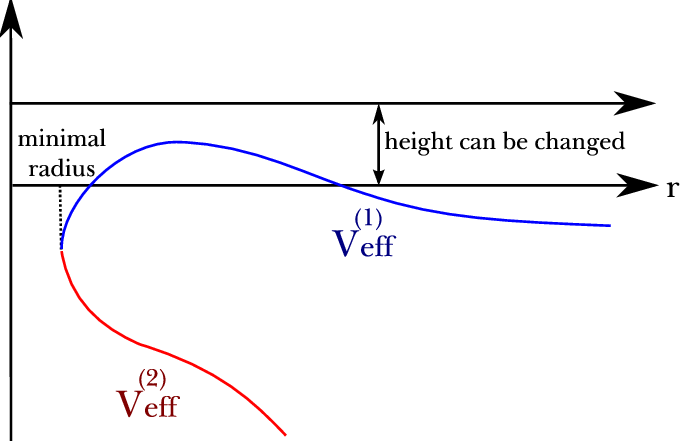
Second, we test the $\Phi_{-}<1$ case. We used $l=2$, $M=0.5$, $\sigma=0.01$, and $\Delta\Phi=0.001$ (i.e., $\Phi_{-}=0.999$). We observe effective potentials $V_{\mathrm{eff}}^{(1)}$ and $V_{\mathrm{eff}}^{(2)}$, as shown in Figure 5. Also, we test $l=2$, $M=0.5$, $\sigma=0.1$, and $\Delta\Phi=0.001$ (i.e., $\Phi_{-}=0.999$), as shown in Figure 6. The effective potentials $V_{\mathrm{eff}}^{(1,2)}$ are convex functions (lower right of Figure 5).

These effective potentials allow a collapsing solution or an expanding solution. Then, there are basically five possibilities: (a) from expanding to collapsing, (b) from collapsing to expanding, (c) from collapsing to collapsing, (d) from expanding to expanding, and (e) a static solution in an unstable equilibrium. (a) and (b) are symmetric solutions, whereas (c) and (d) are asymmetric solutions. For simplicity, we omit the unstable equilibrium case (e). Note that $V_{\mathrm{eff}}^{(2)}$ is only for asymmetric solutions.

Using the information for effective potentials, we know information for $\dot{r}^{2}$. Now we have to know further about the sign of $\epsilon_{\pm}$ to determine causal structures. Especially, the sign of $\epsilon_{-}$ is not entirely clear since it is combined with $\bar{\sigma}$. As in Einstein gravity, we define the effective extrinsic curvatures by the following form [12, 13, 25]:

$\displaystyle\beta^{(i)}_{-}=\frac{f_{-}-f_{+}+16\pi^{2}{\sigma^{(i)}_{\mathrm{eff}}}^{2}r^{2}}{8\pi r\sigma^{(i)}_{\mathrm{eff}}}=\pm\sqrt{-2V^{(i)}_{\mathrm{eff}}+f_{-}}$

(51)

and

$\displaystyle\beta^{(i)}_{+}=\frac{f_{-}-f_{+}-16\pi^{2}{\sigma^{(i)}_{\mathrm{eff}}}^{2}r^{2}}{8\pi r\sigma^{(i)}_{\mathrm{eff}}}=\pm\sqrt{-2V^{(i)}_{\mathrm{eff}}+f_{+}},$

(52)

where we define the effective tension

$\displaystyle\sigma^{(i)}_{\mathrm{eff}}=\sigma+\bar{\sigma}^{(i)},$

(53)

and $i=1,2$ denotes the index of the effective potential $V^{(1)}_{\mathrm{eff}}$ or $V^{(2)}_{\mathrm{eff}}$. The effective extrinsic curvatures do not give direct results for the sign of each root because $\sigma_{\mathrm{eff}}$ already contains $\epsilon_{-}$. However, if we know $\epsilon_{-}$, then we can easily determine $\epsilon_{+}$ from the sign of $\beta_{+}$.

First, we summarize the sign of each root for the inside and the outside of the effective potentials when the effective tensions are always positive.

• •

  $r\sim 0$ limit

  • –

    $\beta_{-}$ is always positive.

  • –

    $\beta_{+}$ is always positive.

• •

  $r\rightarrow\infty$ limit

  • –

    $\beta_{-}$ can be positive or negative for a choice of parameters.

  • –

    $\beta_{+}$ is always negative.

Now we briefly summarize how to determine the sign of $\epsilon_{-}$.

1. 1.

   For the $V^{(1)}_{\mathrm{eff}}$ case, the sign $\epsilon_{\pm}$ will follow the Einstein limit.

   Then, for $\sigma=0.01$, as mentioned in the previous paragraph, the symmetric collapsing solution is $\epsilon_{-}=1$ and the symmetric repulsing solution is $\epsilon_{-}=-1$. For $\sigma=0.1$, $\sqrt{\dot{r}^{2}+f_{-}}$ always has non-zero values, as shown in Figures 8 and 10, and then asymmetric solutions are $\epsilon_{-}=1$ since $\beta^{(1)}_{-}$ cannot change its sign.

   If the effective tension $\sigma^{(1)}_{\mathrm{eff}}$ under previous choices is always positive, our conclusion is self-consistent. We can check from the effective tensions in Figures 11, 12, 13, and 14.

2. 2.

   For the $V^{(2)}_{\mathrm{eff}}$ case, it is entirely unclear whether it will follow the Einstein limit or not. To figure out $\epsilon_{\pm}$, we must first observe whether $\sqrt{\dot{r}^{2}+f_{\pm}}$ become $0$ or not. If they do not become $0$, they will maintain their signs.

   This can be confirmed by looking at the lower left and right of Figures 7, 8, 9, and 10.

3. 3.

   Then, first choose $\epsilon_{-}$, and insert it into $\sigma^{(2)}_{\mathrm{eff}}$. Then, observe $\beta^{(2)}_{\pm}$; if they change their signs, the original choice of $\epsilon_{-}$ was inconsistent. Using this method, we can find a consistent $\epsilon_{-}$.

   If we choose $\epsilon_{-}=+1$ for the $\Phi>1$ case and $\epsilon_{-}=-1$ for the $\Phi<1$ case, we can see that $\beta^{(2)}_{-}$ has consistent signs (Figures 11, 12, 13, and 14). However, if we choose opposite signs for each case, $\beta^{(2)}_{-}$ will change their signs and this situation is inconsistent (Figure 15).

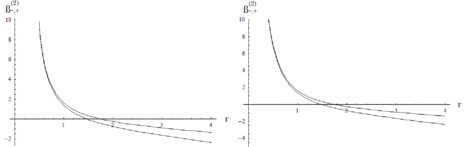
Note that, for $V_{\mathrm{eff}}^{(2)}$, some cases allow a negative tension, as can be seen in the lower right of Figure 11, the lower right of Figure 12, the lower right of Figure 13, and the lower right of Figure 14. These situations correspond to the violation of the null energy condition. Then, the violation of the null energy condition will give new causal structures that were disallowed in pure Einstein theory.

If $\Phi_{-}>1$, for small $r$, there is a radius bound inside of the Schwarzschild radius where the thin shell bubble is not allowed. One may interpret this by saying that if the radius of the shell becomes smaller than the region, the shell should collapse to a singularity, although the thin shell approximation is no more than a good approximation for the region and hence the inside bubble may become an unstable one.

Using the information on the signs of $\epsilon_{\pm}$, we finally classify the causal structures. The following are general rules to determine causal structures [12, 13, 25]:

• •

  $r\sim 0$ limit

  • –

    If $\beta^{(i)}_{-}$ is positive, the outward-pointed normal has to point toward larger $r$; when the shell touches $r\sim 0$ in the de Sitter space, the shell has to touch the left boundary. If $\beta^{(i)}_{-}$ is negative, the shell has to touch the right boundary.

  • –

    If $\beta^{(i)}_{+}$ is positive, when the shell touches $r\sim 0$ in the Schwarzschild space, the shell starting towards the right from the past singularity or moving towards the left before hitting the future singularity is allowed. If $\beta^{(i)}_{+}$ is negative, the opposite behavior will be obtained.

• •

  $r\rightarrow\infty$ limit

  • –

    If $\beta^{(i)}_{-}$ is negative, the shell starts from the past infinity towards the right and ends at the future infinity veering left. If $\beta^{(i)}_{-}$ is positive, the opposite behavior will be obtained.

  • –

    If $\beta^{(i)}_{+}$ is negative, when the shell expands, the shell has to touch the left boundary. If $\beta^{(i)}_{+}$ is positive, when the shell expands, the shell has to touch the right boundary.

First, let us classify the symmetric solutions. The left diagram of Figure 16 is for the de Sitter space, and the right diagram is for the Schwarzschild space. For a collapsing case, $\mathrm{dS}_{\mathrm{A}}$ or $\mathrm{dS}_{\mathrm{D}}$ are possible; and $\mathrm{Sch}_{\mathrm{B}}$, $\mathrm{Sch}_{\mathrm{C}}$, or $\mathrm{Sch}_{\mathrm{D}}$ are possible. Also, for an expanding case, $\mathrm{dS}_{\mathrm{B}}$ or $\mathrm{dS}_{\mathrm{C}}$ are possible; and $\mathrm{Sch}_{\mathrm{A}}$ or $\mathrm{Sch}_{\mathrm{E}}$ are possible. However, according to the behavior of the extrinsic curvatures in $r\rightarrow 0$ or $r\rightarrow\infty$ limit, we can remove the solutions of $\mathrm{dS}_{\mathrm{D}}$, $\mathrm{Sch}_{\mathrm{C}}$, and $\mathrm{Sch}_{\mathrm{E}}$. Also, $\mathrm{dS}_{\mathrm{B}}$ requires $\beta_{-}>0$ in the $r\rightarrow\infty$ limit; however, it requires a sufficiently large tension, and then a symmetric solution will not be allowed. Therefore, there are three possible solutions: $\mathrm{dS}_{\mathrm{A}}-\mathrm{Sch}_{\mathrm{B}}$, $\mathrm{dS}_{\mathrm{A}}-\mathrm{Sch}_{\mathrm{D}}$, and $\mathrm{dS}_{\mathrm{C}}-\mathrm{Sch}_{\mathrm{A}}$. However, these solutions are allowed in pure Einstein gravity.

Second, let us classify the asymmetric solutions (Figure 17). The most interesting case is that of the creation of a bubble universe. In this case, we need to consider the example from an expanding to an expanding solution. Here, $\mathrm{dS}_{\mathrm{E}}$, $\mathrm{dS}_{\mathrm{F}}$ are allowed and, at that time, $\mathrm{Sch}_{\mathrm{F}}$ is allowed for positive tensions. $\mathrm{Sch}_{\mathrm{G}}$ is allowed from $V_{\mathrm{eff}}^{(2)}$ of the $\Phi_{-}>1$ case, but in this case, $\beta^{(2)}_{-}$ is always positive, and, hence, $\mathrm{dS}_{\mathrm{F}}$ corresponds. Also, $\mathrm{dS}_{\mathrm{G}}$ is allowed by $V_{\mathrm{eff}}^{(2)}$ of the $\Phi_{-}<1$ case with negative $\beta^{(2)}_{-}$ and, at that time, $\mathrm{Sch}_{\mathrm{H}}$ is allowed. Thus we have four possible solutions: $\mathrm{dS}_{\mathrm{E}}-\mathrm{Sch}_{\mathrm{F}}$, $\mathrm{dS}_{\mathrm{F}}-\mathrm{Sch}_{\mathrm{F}}$, $\mathrm{dS}_{\mathrm{F}}-\mathrm{Sch}_{\mathrm{G}}$, and $\mathrm{dS}_{\mathrm{G}}-\mathrm{Sch}_{\mathrm{H}}$.

Solutions $\mathrm{dS}_{\mathrm{E}}-\mathrm{Sch}_{\mathrm{G}}$ from $V_{\mathrm{eff}}^{(2)}$ of the $\Phi_{-}>1$ case as well as $\mathrm{dS}_{\mathrm{G}}-\mathrm{Sch}_{\mathrm{H}}$ from $V_{\mathrm{eff}}^{(2)}$ of the $\Phi_{-}<1$ case are new solutions that were disallowed in Einstein gravity. Especially, the former will be useful to discuss the information loss problem. If the bubble becomes larger than the cosmological horizon of the inside de Sitter space, it begins to inflate. Then, there should be a neck of a wormhole on the shell. Although the thin shell approximation cannot describe the throat, it has been demonstrated by numerical simulations by previous authors [29]. We note the causal structures in Figure 18.

As a limiting case, we observe the $\Phi_{-}>1$ and $M=0$ case. We used $l=2$, $M=0$, $\sigma=0.01$, and $\Delta\Phi=0.01$ (i.e., $\Phi_{-}=1.01$) so that

$$\epsilon\sim\frac{(\Delta\Phi)^{2}}{\sigma}\sim 10^{-2}\ll 1\sim l.$$

(54)

Hence, the thin shell approximation holds for these parameters.

We observed effective potentials $V_{\mathrm{eff}}^{(1)}$ and $V_{\mathrm{eff}}^{(2)}$, and the effective tensions $\sigma_{\mathrm{eff}}^{(1)}$ and $\sigma_{\mathrm{eff}}^{(2)}$ (Figure 19). All effective potentials monotonely decrease, so that symmetric bounce solutions are allowed.

We can think that the signs of $\epsilon_{-}$ will follow those of the results of previous sections, $\epsilon^{(1)}_{-}=-1$ and $\epsilon^{(2)}_{-}=+1$. Also, it is not difficult to check by using small and non-zero $M$ and using the previous procedures to determine the sign.

For the potential $V_{\mathrm{eff}}^{(1)}$, the effective tension $\sigma^{(1)}_{\mathrm{eff}}$ converges to a positive value. Then, in the flat background, it cannot touch the right boundary. This implies that such a bubble cannot be described by the thin shell approximation, and that the bubble is unstable [29]. For the potential $V_{\mathrm{eff}}^{(2)}$, the effective tension $\sigma^{(2)}_{\mathrm{eff}}$ converges to a negative value. Then, in the flat background, it can touch the right boundary. Then, we obtain one interesting solution (Figure 20). We obtain $\mathrm{dS}_{\mathrm{B}}-\mathrm{Flat}_{\mathrm{A}}$ since $\beta^{(2)}_{-}$ is always positive; this was disallowed in pure Einstein gravity with the null energy condition.

Note that if we choose $\Phi_{-}<1$, again, only symmetric expanding solutions will be allowed. However, in this case, $\beta_{+}$ should be negative, and, hence, stable solutions are not allowed.

References

- [1] S. Weinberg, “Gravitation and Cosmology,” New York, Wiley (1972).
- [2] C. Brans and C. H. Dicke, Phys. Rev. 124, 925 (1961).
- [3] M. Gasperini, “Elements of string cosmology,” Cambridge, Cambridge University Press (2007).
- [4] L. Randall and R. Sundrum, Phys. Rev. Lett. 83, 3370 (1999) [arXiv:hep-ph/9905221].
- [5] J. Garriga and T. Tanaka, Phys. Rev. Lett. 84, 2778 (2000) [arXiv:hep-th/9911055].
- [6] Y. Fujii and K. Maeda, “The scalar-tensor theory of gravitation,” Cambridge, Cambridge University Press (2003).
- [7]
A. G. Agnese and M. La Camera,
Phys. Rev. D 51, 2011 (1995);
F. He and S.-W. Kim, Phys. Rev. D 65, 084022 (2002);
R. Izmailov, A. Bhattacharya and K. K. Nandi, arXiv:1006.4819 [gr-qc]. - [8]
H. Kim, H. W. Lee, Y. S. Myung, Phys. Lett. B 628, 11-17 (2005) [arXiv:gr-qc/0507010];
M. R. Setare, Phys. Lett. B 644, 99 (2007) [arXiv:hep-th/0610190]. - [9]
W. Israel, Nuovo Cimento 44B, 1, (1966); ibid. 48B, 463(E) (1967);
K. G. Suffern, J. Phys. A 15, 1599 (1982);
V. A. Berezin, V. A. Kuzmin and I. I. Tkachev, Phys. Rev. D 36, 2919 (1987);
P. S. Letelier and A. Wang, Phys. Rev. D 48, 631 (1993). - [10]
M. B. Voloshin, I. Yu. Kobzarev, and L. B. Okun, Yad. Fiz. 20, 1229 (1974) [Sov. J. Nucl. Phys. 20, 644 (1975)];
S. R. Coleman, Phys. Rev. D 15, 2929 (1977) [Erratum-ibid. Phys. Rev. D 16, 1248 (1977)];
C. G. Callan and S. R. Coleman, Phys. Rev. D 16, 1762 (1977);
S. R. Coleman and F. De Luccia, Phys. Rev. D 21, 3305 (1980);
K. M. Lee and E. J. Weinberg, Phys. Rev. D 36, 1088 (1987);
B.-H. Lee and W. Lee, Class. Quant. Grav. 26, 225002 (2009) [arXiv:0809.4907]. - [11]
K. Sato, M. Sasaki, H. Kodama and K. i. Maeda, Prog. Theor. Phys. 65, 1443 (1981);
H. Kodama, M. Sasaki, K. Sato and K. i. Maeda, Prog. Theor. Phys. 66, 2052 (1981);
K. i. Maeda, K. Sato, M. Sasaki and H. Kodama, Phys. Lett. B 108, 98 (1982);
K. Sato, H. Kodama, M. Sasaki and K. i. Maeda, Phys. Lett. B 108, 103 (1982). - [12] S. K. Blau, E. I. Guendelman and A. H. Guth, Phys. Rev. D 35, 1747 (1987).
- [13]
A. Aguirre and M. C. Johnson, Phys. Rev. D 72, 103525 (2005) [arXiv:gr-qc/0508093];
A. Aguirre and M. C. Johnson, Phys. Rev. D 73, 123529 (2006) [arXiv:gr-qc/0512034];
V.I. Dokuchaev, S.V. Chernov, Class. Quant. Grav. 25, 015004 (2008) [arXiv:0709.0616 [gr-qc]];
F.-L. Lin, C.-H. Wang, C.-P. Yeh, [arXiv:1003.4402]. - [14]
G. L. Alberghi, D. A. Lowe and M. Trodden, JHEP 9907, 020 (1999) [arXiv:gr-qc/9906047];
G. Arreaga, I. Cho, J. Guven, Phys. Rev. D 62, 043520 (2000) [arXiv:gr-qc/0001078];
B.-H. Lee, W. Lee, S. Nam, and C. Park, Phys. Rev. D 75, 103506 (2007) [arXiv:hep-th/0701210];
V.I. Dokuchaev, S.V. Chernov, J. Exp. Theor. Phys. 110, 7 (2010) [arXiv:1002.4602]. - [15] H. A. Chamblin and H. S. Reall, Nucl. Phys. B 562, 133 (1999).
- [16]
D. S. Goldwirth and H. W. Zaglauer, Phys. Rev. Lett. 67, 3639 (1991);
N. Sakai and K.-i. Maeda, Phys. Rev. D 48, 5570 (1993). - [17] D. Hwang and D. Yeom, Class. Quant. Grav. 27, 205002 (2010) [arXiv:1002.4246].
- [18] W. Lee, B. H. Lee, C. H. Lee and C. Park, Phys. Rev. D 74, 123520 (2006) [arXiv:hep-th/0604064].
- [19] B. H. Lee, C. H. Lee, W. Lee, S. Nam and C. Park, Phys. Rev. D 77, 063502 (2008) [arXiv:0710.4599 [hep-th]].
- [20] B. H. Lee, C. H. Lee, W. Lee, S. Nam and C. Park, J. Korean Phys. Soc. 53, 1101 (2008), (The figure 2 has need to be replaced with 5, 3 with 6, and 4 with 7, without replacing figure captions in the paper.)
- [21] E. I. Guendelman and N. Sakai, Phys. Rev. D 77, 125002 (2008).
- [22] H. Kim, Phys. Rev. D 60, 024001 (1999).
- [23] E. Farhi and A. H. Guth, Phys. Lett. B 183, 149 (1987).
- [24]
E. Farhi, A. H. Guth and J. Guven, Nucl. Phys. B 339, 417 (1990);
W. Fischler, D. Morgan and J. Polchinski, Phys. Rev. D 41, 2638 (1990);
W. Fischler, D. Morgan and J. Polchinski, Phys. Rev. D 42, 4042 (1990). - [25] B. Freivogel, V. E. Hubeny, A. Maloney, R. C. Myers, M. Rangamani and S. Shenker, JHEP 0603, 007 (2006) [arXiv:hep-th/0510046].
- [26] H. Kim, B. H. Lee, W. Lee, Y. J. Lee and D. Yeom, arXiv:1011.5981 [hep-th].
- [27]
J. W. York, Phys. Rev. Lett. 28, 1082 (1972);
G. W. Gibbons and S. W. Hawking, Phys. Rev. D 15, 2752 (1977). - [28] C. W. Misner, K. S. Thorne and J. A. Wheeler, “Gravitation,” San Francisco, Freeman (1973).
- [29] J. Hansen, D. Hwang and D. Yeom, JHEP 0911, 016 (2009) [arXiv:0908.0283 [gr-qc]].
- [30] B. Bertotti, L. Iess and P. Tortora, Nature 425, 374 (2003).
- [31] J. Khoury and A. Weltman, Phys. Rev. Lett. 93, 171104 (2004) [arXiv:astro-ph/0309300].
- [32] D. Yeom, arXiv:0912.0068 [gr-qc].
- [33]
J. M. Maldacena, Adv. Theor. Math. Phys. 2, 231 (1998) [Int. J. Theor. Phys. 38, 1113 (1999)] [arXiv:hep-th/9711200];
E. Witten, Adv. Theor. Math. Phys. 2, 253 (1998) [arXiv:hep-th/9802150];
S. S. Gubser, I. R. Klebanov and A. M. Polyakov, Phys. Lett. B 428, 105 (1998) [arXiv:hep-th/9802109];
A. Strominger, JHEP 0110, 034 (2001) [arXiv:hep-th/0106113]. - [34] S. W. Hawking, Phys. Rev. D 14, 2460 (1976).