A drift homotopy Monte Carlo approach to particle filtering for multi-target tracking

Vasileios Maroulas Affiliation: Department of Mathematics Affiliation: University of Tennessee Affiliation: Knoxville, TN 37996 Affiliation: and Affiliation: Panos Stinis Affiliation: Department of Mathematics Affiliation: University of Minnesota Affiliation: Minneapolis, MN 55455

Abstract

We present a novel approach for improving particle filters for multi-target tracking. The suggested approach is based on drift homotopy for stochastic differential equations. Drift homotopy is used to design a Markov Chain Monte Carlo step which is appended to the particle filter and aims to bring the particle filter samples closer to the observations. Also, we present a simple Metropolis Monte Carlo algorithm for tackling the target-observation association problem. We have used the proposed approach on the problem of multi-target tracking for both linear and nonlinear observation models. The numerical results show that the suggested approach can improve significantly the performance of a particle filter.

Introduction

Multi-target tracking is a central and difficult problem arising in many scientific and engineering applications including radar and signal processing, air traffic control and GPS navigation [11]. The tracking problem consists of computing the best estimate of the targets’ trajectories based on noisy measurements (observations).

Several strategies have been developed for addressing the multi-target tracking problem, see e.g. [1, 6, 5, 14, 8, 10, 11, 12, 13, 19]. In this paper we focus on particle filter techniques [5, 14]. The popularity of the particle filter method has increased due to its flexibility to handle cases where the dynamic and observation models are non-linear and/or non-Gaussian. The particle filter approach is an importance sampling method which approximates the target distribution by a discrete set of weighted samples (particles). The weights of the samples are updated when observations become available in order to incorporate information from the observations.

Despite the particle filter’s flexibility, it is often found in practice that most samples will have a negligible weight with respect to the observation, in other words their corresponding contribution to the target distribution will be negligible. Therefore, one may resample the weights to create more copies of the samples with significant weights [8]. However, even with the resampling step, the particle filter might still need a lot of samples in order to approximate accurately the target distribution. Typically, a few samples dominate the weight distribution, while the rest of the samples are in statistically insignificant regions. Thus, some authors (see e.g. [7, 20]) have suggested the use of an extra step, after the resampling step, which can help move more samples in statistically significant regions.

The extra step for the particle filter is a problem of conditional path sampling for stochastic differential equations (SDEs). In [16], a new approach to conditional path sampling was presented. In that paper, it was also shown how the algorithm can be used to perform the extra step of a particle filter. In the current work, we have applied the conditional path sampling algorithm from [16] to perform the extra step of a particle filter for the problem of multi-target tracking.

The suggested approach is based on drift homotopy for the SDE system which describes the dynamics of the targets. The dynamics of an SDE are governed by a deterministic term, called the drift, and a stochastic term, called the noise. While unconditional path sampling is straightforward for SDEs, albeit expensive for high dimensional systems, conditional path sampling can be difficult even for low dimensional systems. On the other hand, it can be easier to find conditional paths for an SDE with a modified drift which is usually simpler than the drift of the original equation. Of course, these simplified paths may have a very low probability of being paths of the original SDE. Drift homotopy proceeds by considering a sequence of SDEs with drifts which interpolate between the original and modified drifts. Then one samples (through MCMC sampling) paths from each SDE in the sequence using the best sample from the previous SDE in the sequence as the initial condition for the MCMC sampling. This allows one to gradually morph a path of the modified SDE (which maybe easier to satisfy the conditions) to a conditional path of the original SDE.

In addition to the extra step for the particle filter, we have designed and implemented a simple Metropolis Monte Carlo algorithm for the target-observation association problem. This algorithm effects a probabilistic search of the space of possible associations to find the best target-observation association. Of course, one can use more sophisticated association algorithms (see [14] and references therein) but the Monte Carlo algorithm performed very well in the numerical experiments.

This paper is organized as follows. Sections 1.1 and 1.2 provide a brief presentation of particle filters for single and multiple targets (more details can be found in [8, 5, 9, 14]), which will serve to highlight the versatility and drawbacks of this popular filtering method. Sections 1.3 and 1.4 demonstrate how one can use an extra step to improve the performance of particle filters for single and multiple targets. In particular, we discuss how drift homotopy can be used to effect the extra step. Section 2 describes the Monte Carlo sampling algorithm for computing the best association between observations and targets for the case of multiple targets. Section 3 presents numerical results for multi-target tracking for the cases of linear and nonlinear observation models. Finally, Section 4 contains a discussion of the results as well as directions for future work.

1 Particle filtering

Particle filters are a special case of sequential importance sampling methods. In Sections 1.1 and 1.2 we discuss the generic particle filter for a single and multiple targets respectively. In Sections 1.3 and 1.4 we discuss the addition of an extra step to the generic particle filter for the cases of a single and multiple targets respectively.

1.1 Generic particle filter for a single target

Suppose that we are given an SDE system and that we also have access to noisy observations $Z_{T_{1}},\ldots,Z_{T_{K}}$ of the state of the system at specified instants $T_{1},\ldots,T_{K}.$ The observations are functions of the state of the system, say given by $Z_{T_{k}}=G(X_{T_{k}},\xi_{k}),$ where $\xi_{k},k=1,\ldots,K$ are mutually independent random variables. For simplicity, let us assume that the distribution of the observations admits a density $g(X_{T_{k}},Z_{T_{k}}),$ i.e., $p(Z_{T_{k}}|X_{T_{k}})\propto g(X_{T_{k}},Z_{T_{k}}).$

The filtering problem consists of computing estimates of the conditional expectation $E[f(X_{T_{k}})|\{Z_{T_{j}}\}^{k}_{j=1}],$ i.e., the conditional expectation of the state of the system given the (noisy) observations. Equivalently, we are looking to compute the conditional density of the state of the system given the observations $p(X_{T_{k}}|\{Z_{T_{j}}\}^{k}_{j=1}).$ There are several ways to compute this conditional density and the associated conditional expectation but for practical applications they are rather expensive.

Particle filters fall in the category of importance sampling methods. Because computing averages with respect to the conditional density involves the sampling of the conditional density which can be difficult, importance sampling methods proceed by sampling a reference density $q(X_{T_{k}}|\{Z_{T_{j}}\}^{k}_{j=1})$ which can be easily sampled and then compute the weighted sample mean

E[f(X_{T_{k}})|\{Z_{T_{j}}\}^{k}_{j=1}]\approx\frac{1}{N}\sum_{n=1}^{N}f(X^{n}_{T_{k}})\frac{p(X^{n}_{T_{k}}|\{Z_{T_{j}}\}^{k}_{j=1})}{q(X^{n}_{T_{k}}|\{Z_{T_{j}}\}^{k}_{j=1})}

or the related estimate

E[f(X_{T_{k}})|\{Z_{T_{j}}\}^{k}_{j=1}]\approx\frac{\sum_{n=1}^{N}f(X^{n}_{T_{k}})\frac{p(X^{n}_{T_{k}}|\{Z_{T_{j}}\}^{k}_{j=1})}{q(X^{n}_{T_{k}}|\{Z_{T_{j}}\}^{k}_{j=1})}}{\sum_{n=1}^{N}\frac{p(X^{n}_{T_{k}}|\{Z_{T_{j}}\}^{k}_{j=1})}{q(X^{n}_{T_{k}}|\{Z_{T_{j}}\}^{k}_{j=1})}},

(1)

where $N$ has been replaced by the approximation

N\approx\sum_{n=1}^{N}\frac{p(X^{n}_{T_{k}}|\{Z_{T_{j}}\}^{k}_{j=1})}{q(X^{n}_{T_{k}}|\{Z_{T_{j}}\}^{k}_{j=1})}.

Particle filtering is a recursive implementation of the importance sampling approach. It is based on the recursion

	$\displaystyle p(X_{T_{k}}\|\{Z_{T_{j}}\}^{k}_{j=1})$	$\displaystyle\propto g(X_{T_{k}},Z_{T_{k}})p(X_{T_{k}}\|\{Z_{T_{j}}\}^{k-1}_{j=1}),$		(2)
	$\displaystyle\text{where}\;\;p(X_{T_{k}}\|\{Z_{T_{j}}\}^{k-1}_{j=1})$	$\displaystyle=\int p(X_{T_{k}}\|X_{T_{k-1}})p(X_{T_{k-1}}\|\{Z_{T_{j}}\}^{k-1}_{j=1})dX_{T_{k-1}}.$		(3)

If we set

q(X_{T_{k}}|\{Z_{T_{j}}\}^{k}_{j=1})=p(X_{T_{k}}|\{Z_{T_{j}}\}^{k-1}_{j=1}),

then from (2) we get

\frac{p(X_{T_{k}}|\{Z_{T_{j}}\}^{k}_{j=1})}{q(X_{T_{k}}|\{Z_{T_{j}}\}^{k}_{j=1})}\propto g(X_{T_{k}},Z_{T_{k}}).

The approximation in expression (1) becomes

E[f(X_{T_{i}})|\{Z_{T_{j}}\}^{k}_{j=1}]\approx\frac{\sum_{n=1}^{N}f(X^{n}_{T_{k}})g(X^{n}_{T_{k}},Z_{T_{k}})}{\sum_{n=1}^{N}g(X^{n}_{T_{k}},Z_{T_{k}})}

(4)

From (4) we see that if we can construct samples from the predictive distribution $p(X_{T_{k}}|\{Z_{T_{j}}\}^{k-1}_{j=1})$ then we can define the (normalized) weights $W^{n}_{T_{k}}=\frac{g(X^{n}_{T_{k}},Z_{T_{k}})}{\sum_{n=1}^{N}g(X^{n}_{T_{k}},Z_{T_{k}})},$ use them to weigh the samples and the weighted samples will be distributed according to the posterior distribution $p(X_{T_{k}}|\{Z_{T_{j}}\}^{k}_{j=1}).$

In many applications, most samples will have a negligible weight with respect to the observation, so carrying them along does not contribute significantly to the conditional expectation estimate (this is the problem of degeneracy [9]). To create larger diversity one can resample the weights to create more copies of the samples with significant weights. The particle filter with resampling is summarized in the following algorithm due to Gordon et al. [8].

Particle filter for a single target

1.

Begin with $N$ unweighted samples $X^{n}_{T_{k-1}}$ from $p(X_{T_{k-1}}|\{Z_{T_{j}}\}^{k-1}_{j=1}).$
2.

Prediction: Generate $N$ samples $X^{\prime n}_{T_{k}}$ from $p(X_{T_{k}}|X_{T_{k-1}}).$
3.

Update: Evaluate the weights

$W^{n}_{T_{k}}=\frac{g(X^{\prime n}_{T_{k}},Z_{T_{k}})}{\sum_{n=1}^{N}g(X^{\prime n}_{T_{k}},Z_{T_{k}})}.$
4.

Resampling: Generate $N$ independent uniform random variables $\{\theta^{n}\}_{n=1}^{N}$ in $(0,1).$ For $n=1,\ldots,N$ let $X^{n}_{T_{k}}=X^{\prime j}_{T_{k}}$ where

$\sum_{l=1}^{j-1}W^{l}_{T_{k}}\leq\theta^{j}<\sum_{l=1}^{j}W^{l}_{T_{k}}$

where $j$ can range from $1$ to $N.$
5.

Set $k=k+1$ and proceed to Step 1.

The particle filter algorithm is easy to implement and adapt for different problems since the only part of the algorithm that depends on the specific dynamics of the problem is the prediction step. This has led to the particle filter algorithm’s increased popularity [5]. However, even with the resampling step, the particle filter can still need a lot of samples in order to describe accurately the conditional density $p(X_{T_{k}}|\{Z_{T_{j}}\}^{k}_{j=1}).$ Snyder et al. [15] have shown how the particle filter can fail in simple high dimensional problems because one sample dominates the weight distribution. The rest of the samples are not in statistically significant regions. Even worse, as we will show in the numerical results section, there are simple examples where not even one sample is in a statistically significant region. In the next subsection we present how drift homotopy can be used to push samples closer to statistically significant regions.

1.2 Generic particle filter for multiple targets

Suppose that we have $\lambda=1,\ldots,\Lambda$ targets. Also, for notational simplicity, assume that the $\lambda$ th target comes from the $\lambda$ th observation. Even when this is not the case, we can relabel the observations to satisfy this assumption. We will discuss in Section 2 how targets can be associated to observations. The targets are assumed to evolve independently so that the observation weight of a sample of the vector of targets is the product of the individual observation weights of the targets [14]. The same is true for the transition density of the vector of targets between observations. We denote the vector of targets at observation $T_{k}$ by

X_{T_{k}}=(X_{1,T_{k}},\ldots,X_{\Lambda,T_{k}})

and the observation vector at $T_{k}$ by

Z_{T_{k}}=(Z_{1,T_{k}},\ldots,Z_{\Lambda,T_{k}}).

Also, we can have different observation weight densities $g_{\lambda},\;\lambda=1,\ldots,\Lambda$ for different targets. However, in the numerical examples we have chosen the same observation weight density for all targets.

Following [14] we can write the particle filter for the case of multiple targets as

Particle filter for multiple targets

1.

Begin with $N$ unweighted samples $X^{n}_{T_{k-1}}$ from $p(X_{T_{k-1}}|\{Z_{T_{j}}\}^{k-1}_{j=1})=\prod_{\lambda=1}^{\Lambda}p(X_{\lambda,T_{k-1}}|\{Z_{\lambda,T_{j}}\}^{k-1}_{j=1}).$
2.

Prediction: Generate $N$ samples $X^{\prime n}_{T_{k}}$ from

$p(X_{T_{k}}|X_{T_{k-1}})=\prod_{\lambda=1}^{\Lambda}p(X_{\lambda,T_{k}}|X_{\lambda,T_{k-1}}).$

Update: Evaluate the weights

W^{n}_{T_{k}}=\frac{\prod_{\lambda=1}^{\Lambda}g_{\lambda}({X^{\prime}}^{n}_{\lambda,T_{k}},Z_{\lambda,T_{k}})}{\sum_{n=1}^{N}\prod_{\lambda=1}^{\Lambda}g_{\lambda}({X^{\prime}}^{n}_{\lambda,T_{k}},Z_{\lambda,T_{k}})}.

4.

Resampling: Generate $N$ independent uniform random variables $\{\theta^{n}\}_{n=1}^{N}$ in $(0,1).$ For $n=1,\ldots,N$ let $X^{n}_{T_{k}}=X^{\prime j}_{T_{k}}$ where

$\sum_{l=1}^{j-1}W^{l}_{T_{k}}\leq\theta^{j}<\sum_{l=1}^{j}W^{l}_{T_{k}}$

where $j$ can range from $1$ to $N.$
5.

Set $k=k+1$ and proceed to Step 1.

1.3 Particle filter with MCMC step for a single target

Several authors (see e.g. [7, 20]) have suggested the use of a MCMC step after the resampling step (Step 4) in order to move samples away from statistically insignificant regions. There are many possible ways to append an MCMC step after the resampling step in order to achieve that objective. The important point is that the MCMC step must preserve the conditional density $p(X_{T_{k}}|\{Z_{T_{j}}\}^{k}_{j=1}).$ In the current section we show that the MCMC step constitutes a case of conditional path sampling.

We begin by noting that one can use the resampling step (Step 4) in the particle filter algorithm to create more copies not only of the good samples according to the observation, but also of the values (initial conditions) of the samples at the previous observation. These values are the ones who have evolved into good samples for the current observation (see more details in [20]). The motivation behind producing more copies of the pairs of initial and final conditions is to use the good initial conditions as starting points to produce statistically more significant samples according to the current observation. This process can be accomplished in two steps. First, Step 4 of the particle filter algorithm is replaced by

Resampling: Generate $N$ independent uniform random variables $\{\theta^{n}\}_{n=1}^{N}$ in $(0,1).$ For $n=1,\ldots,N$ let $(X^{n}_{T_{k-1}},X^{n}_{T_{k}})=(X^{\prime j}_{T_{k-1}},X^{\prime j}_{T_{k}})$ where

\sum_{l=1}^{j-1}W^{l}_{T_{k}}\leq\theta^{j}<\sum_{l=1}^{j}W^{l}_{T_{k}}

Also, through Bayes’ rule [20] one can show that the posterior density $p(X_{T_{k}}|\{Z_{T_{j}}\}^{k}_{j=1})$ is preserved if one samples from the density

g(X_{T_{k}},Z_{T_{k}})p(X_{T_{k}}|X_{T_{k-1}})

where $X_{T_{k-1}}$ are given by the modified resampling step. This is a problem of conditional path sampling for (continuous-time or discrete) stochastic systems. The important issue is to perform the necessary sampling efficiently [4, 20].

We propose to do that here using drift homotopy. In particular, suppose that we are given a system of stochastic differential equations (SDEs)

dX_{t}=a(X_{t})dt+\sigma(X_{t})dB_{t},

(5)

Also consider an SDE system with modified drift

dY_{t}=b(Y_{t})dt+\sigma(Y_{t})dB_{t},

(6)

where $b(Y_{t})$ is suitably chosen to facilitate the conditional path sampling problem.

Consider a collection of $L+1$ modified SDE systems

dY^{l}_{t}=(1-\epsilon_{l})b(Y^{l}_{t})dt+\epsilon_{l}a(Y^{l}_{t})dt+\sigma(Y^{l}_{t})dB_{t},

where $\epsilon_{l}\in[0,1],\;l=0,\ldots,L,$ with $\epsilon_{l}<\epsilon_{l+1},$ $\epsilon_{0}=0$ and $\epsilon_{L}=1.$ Instead of sampling directly from the density $g(X_{T_{k}},Z_{T_{k}})p(X_{T_{k}}|X_{T_{k-1}}),$ one can sample from the density $g(Y^{0}_{T_{k}},Z_{T_{k}})p(Y^{0}_{T_{k}}|X_{T_{k-1}})$ and gradually morph the sample into a sample of $g(X_{T_{k}},Z_{T_{k}})p(X_{T_{k}}|X_{T_{k-1}})$ .

Drift homotopy algorithm:

•

( $l=0$ ) Begin with a sample from the modified SDE (6).
•

Sample through MCMC the density $g(Y^{0}_{T_{k}},Z_{T_{k}})p(Y^{0}_{T_{k}}|X_{T_{k-1}}).$
•

For $l=1,...,L$ take the last sample from the ( $l-1$ )st SDE and use it as in initial condition for MCMC sampling of the density

$g(Y^{l}_{T_{k}},Z_{T_{k}})p(Y^{l}_{T_{k}}|X_{T_{k-1}})$

at the $l$ th level.
•

Keep the last sample at the $L$ th level.

The drift homotopy algorithm is similar to Simulated Annealing (SA) used in equilibrium statistical mechanics [9]. However, instead of modifying a temperature as in SA, here we modify the drift of the system.

We are now in a position to present the particle filter with MCMC step algorithm

Particle filter with MCMC step for a single target

1.

Begin with $N$ unweighted samples $X^{n}_{T_{k-1}}$ from $p(X_{T_{k-1}}|\{Z_{T_{j}}\}^{k-1}_{j=1}).$
2.

Prediction: Generate $N$ samples $X^{\prime n}_{T_{k}}$ from $p(X_{T_{k}}|X_{T_{k-1}}).$
3.

Update: Evaluate the weights

$W^{n}_{T_{k}}=\frac{g(X^{\prime n}_{T_{k}},Z_{T_{k}})}{\sum_{n=1}^{N}g(X^{\prime n}_{T_{k}},Z_{T_{k}})}.$
4.

Resampling: Generate $N$ independent uniform random variables $\{\theta^{n}\}_{n=1}^{N}$ in $(0,1).$ For $n=1,\ldots,N$ let $(X^{n}_{T_{k-1}},X^{n}_{T_{k}})=(X^{\prime j}_{T_{k-1}},X^{\prime j}_{T_{k}})$ where

$\sum_{l=1}^{j-1}W^{l}_{T_{k}}\leq\theta^{j}<\sum_{l=1}^{j}W^{l}_{T_{k}}$

where $j$ can range from $1$ to $N.$
5.

MCMC step: For $n=1,\ldots,N$ choose a modified drift (possibly different for each $n$ ). Construct a path for the SDE with the modified drift starting from $X^{n}_{T_{k-1}}.$ Construct through drift homotopy a Markov chain for $Y^{n}_{T_{k}}$ with stationary distribution

$g(Y^{n}_{T_{k}},Z_{T_{k}})p(Y^{n}_{T_{k}}|X^{n}_{T_{k-1}})$
6.

Set $X^{n}_{T_{k}}=Y^{n}_{T_{k}}.$
7.

Set $k=k+1$ and proceed to Step 1.

Since the samples $X^{n}_{T_{k}}=Y^{n}_{T_{k}}$ are constructed by starting from different sample paths, they are independent. Also, note that the samples $X^{n}_{T_{k}}$ are unweighted. However, we can still measure how well these samples approximate the posterior density by comparing the effective sample sizes of the particle filter with and without the MCMC step. For a collection of $N$ samples the effective sample size $ess(T_{k})$ is defined by

ess(T_{k})=\frac{N}{1+C_{k}^{2}}

where

C_{k}=\frac{1}{W_{k}}\sqrt{\frac{1}{N}\sum_{n=1}^{N}(g(X^{n}_{T_{k}},Z_{T_{k}})-W_{k})^{2}}\;\;\text{and}\;\;W_{k}=\frac{1}{N}\sum_{n=1}^{N}g(X^{n}_{T_{k}},Z_{T_{k}}).

The effective sample size can be interpreted as that the $N$ weighted samples are worth of $ess(T_{k})=\frac{N}{1+C_{k}^{2}}$ i.i.d. samples drawn from the target density, which in our case is the posterior density. By definition, $ess(T_{k})\leq N.$ If the samples have uniform weights, then $ess(T_{k})=N.$ On the other hand, if all samples but one have zero weights, then $ess(T_{k})=1.$

1.4 Particle filter with MCMC step for multiple targets

We discuss now the case of multiple, say $\Lambda,$ targets. Instead of the observations for a single target now we have a collection of observations for all the targets $\{Z_{T_{j}}\}^{k}_{j=1}=\{(Z^{1}_{T_{j}},\ldots,Z^{\lambda}_{T_{j}})\}^{k}_{j=1}.$

The particle filter with MCMC step for the case of multiple targets is

Particle filter with MCMC step for multiple targets

1.

Begin with $N$ unweighted samples $X^{n}_{T_{k-1}}$ from $p(X_{T_{k-1}}|\{Z_{T_{j}}\}^{k-1}_{j=1})=\prod_{\lambda=1}^{\Lambda}p(X_{\lambda,T_{k-1}}|\{Z_{\lambda,T_{j}}\}^{k-1}_{j=1}).$
2.

Prediction: Generate $N$ samples $X^{\prime n}_{T_{k}}$ from

$p(X_{T_{k}}|X_{T_{k-1}})=\prod_{\lambda=1}^{\Lambda}p(X_{\lambda,T_{k}}|X_{\lambda,T_{k-1}}).$

Update: Evaluate the weights

W^{n}_{T_{k}}=\frac{\prod_{\lambda=1}^{\Lambda}g_{\lambda}({X^{\prime}}^{n}_{\lambda,T_{k}},Z_{\lambda,T_{k}})}{\sum_{n=1}^{N}\prod_{\lambda=1}^{\Lambda}g_{\lambda}({X^{\prime}}^{n}_{\lambda,T_{k}},Z_{\lambda,T_{k}})}.

4.

Resampling: Generate $N$ independent uniform random variables $\{\theta^{n}\}_{n=1}^{N}$ in $(0,1).$ For $n=1,\ldots,N$ let $(X^{n}_{T_{k-1}},X^{n}_{T_{k}})=(X^{\prime j}_{T_{k-1}},X^{\prime j}_{T_{k}})$ where

$\sum_{l=1}^{j-1}W^{l}_{T_{k}}\leq\theta^{j}<\sum_{l=1}^{j}W^{l}_{T_{k}}$

where $j$ can range from $1$ to $N.$
5.

MCMC step: For $n=1,\ldots,N$ and $\lambda=1,\ldots,\Lambda$ choose a modified drift (possibly different for each $n$ and each $\lambda$ ). Construct a path for the SDE with the modified drift starting from $X^{n}_{\lambda,T_{k-1}}.$ Construct through drift homotopy a Markov chain for $Y^{n}_{T_{k}}$ with stationary distribution

$\prod_{\lambda=1}^{\Lambda}g_{\lambda}(Y^{n}_{\lambda},Z_{\lambda,T_{k}})p_{\lambda}(Y^{n}_{\lambda}|X^{n}_{{\lambda},T_{k-1}}).$
6.

Set $X^{n}_{T_{k}}=Y^{n}_{T_{k}}.$
7.

Set $k=k+1$ and proceed to Step 1.

For a collection of $N$ samples the effective sample size $ess_{\Lambda}(T_{k})$ for $\Lambda$ targets is

ess_{\Lambda}(T_{k})=\frac{N}{1+C_{\Lambda,k}^{2}}

where

C_{\Lambda,k}=\frac{1}{W_{\Lambda,k}}\sqrt{\frac{1}{N}\sum_{n=1}^{N}(\prod_{\lambda=1}^{\Lambda}g_{\lambda}(X^{n}_{\lambda,T_{k}},Z_{\lambda,T_{k}})-W_{\Lambda,k})^{2}}\\ \text{and}\;\;W_{\Lambda,k}=\frac{1}{N}\sum_{n=1}^{N}\prod_{\lambda=1}^{\Lambda}g_{\lambda}(X^{n}_{\lambda,T_{k}},Z_{\lambda,T_{k}}).

2 Monte Carlo target-observation association algorithm

As in any other sequential Monte Carlo algorithm for multi-target tracking (see e.g. [14] and references therein) we need to associate, for each sample, the evolving targets to the observations. The association problem is sensitive to the tracking accuracy of the algorithm. If we cannot follow accurately each target and two or more targets are close, then the association algorithm can assign the wrong observations to the targets. After a few observation steps this can lead to the inability to follow a target’s true track anymore. There are different ways to perform the target-observation association. The ones that we are aware of are based on various types of assignment algorithms first developed in the context of computer science [3, 2]. Here we have decided on using a different algorithm to perform the target-observation association. In particular, we have designed a simple Metropolis Monte Carlo algorithm which effects a probabilistic search of the space of possible associations to find the best target-observation association.

Suppose that at observation time $t$ we have $\Lambda_{t}$ observations which include surviving and possible newborn targets. Also, suppose that for each target we have at each step $J$ observation values for different quantities depending on the target’s state. For simplicity, we assume that we observe the same quantities for all targets. Usually, one observes position related quantities, like the $x,y$ position or the bearing and range of the target. The observation model is given by

Z_{\lambda,j,t}=g_{j}({\bf{x}}_{\lambda,t})+\xi_{\lambda,j},\;\;\text{for}\;\;\lambda=1,\ldots,\Lambda_{t}\;\;\text{and}\;\ j=1,\ldots,J,

(7)

where $\text{for}\;\;\lambda=1,\ldots,\Lambda_{t}\;\;\text{and}\;\ j=1,\ldots,J,\xi_{\lambda,j},$ are i.i.d. random variables. For simplicity let us assume that the $\xi_{\lambda,j}$ are $\sim N(0,\sigma^{2}_{j}).$ Note that the observation model (7) assumes that we know that the $\lambda$ th observation comes from the $\lambda$ th target. However, in reality, we do not have such information and we need to make an association between observations and targets. Define an association map $A$ given by $A(\lambda)=m_{\lambda}$ where $\lambda,m_{\lambda}=1,\ldots,\Lambda_{t}.$ The association map assigns to the $\lambda$ th observation the $m_{\lambda}$ th target. For $\Lambda_{t}$ observations there are $\Lambda_{t}!$ different observation-target association maps. For a specific association of each observation to some target, the likelihood function for the collection of observations for the $n$ th sample is given by

\rho({\bf{x}}^{n}_{1,t},\ldots,{\bf{x}}^{n}_{\Lambda_{t},t},Z_{1,1,t},\ldots,Z_{1,J,t},\ldots,Z_{\Lambda_{t},J,t})\\ \propto\prod_{\lambda=1}^{\Lambda_{t}}\prod_{j=1}^{J}\exp\biggl[-\frac{(Z_{\lambda,j,t}-h_{j}({\bf{x}}_{A(\lambda),t}^{n}))^{2}}{2*\sigma^{2}_{j}}\biggl]

(8)

where the proportionality is up to an (immaterial for our purposes) normalization constant. If we define

H^{A}_{obs}({\bf{x}}^{n}_{1,t},\ldots,{\bf{x}}^{n}_{\Lambda_{t},t},Z_{1,1,t},\ldots,Z_{1,J,t},\ldots,Z_{\Lambda_{t},J,t})\\ =\sum_{\lambda=1}^{\Lambda_{t}}\sum_{j=1}^{J}\frac{(Z_{\lambda,j,t}-h_{j}({\bf{x}}_{A(\lambda),t}^{n}))^{2}}{2*\sigma^{2}_{j}}

we can rewrite $\rho$ (omitting all the arguments of $\rho$ and $H^{A}_{obs}$ for simplicity) as

\rho\propto\exp[-H^{A}_{obs}]

(9)

The superscript $A$ is to denote the dependence of the value of $H^{A}_{obs}$ on the specific association map $A.$ The best association map is the one which maximizes $\rho.$ By definition, $H^{A}_{obs}\geq 0$ and thus the best association is the one which minimizes $H^{A}_{obs}.$ We can find the best association map by standard Metropolis Monte Carlo sampling on the space of association maps, using the density $\rho$ (see e.g. [9] about Metropolis Monte Carlo sampling).

As in every Metropolis Monte Carlo sampling algorithm there is arbitrariness in the new configuration (association map in our case) proposal. We have tried two different proposal schemes which performed equally well, at least for cases up to 4 targets that we examined in our numerical experiments. The first proposal scheme constructs a new observation-target association map from scratch. This means that for each observation in the observation vector we choose a new target to associate it with. Note that if there is only one target there is no need for sampling since there is only one possible observation-target association. The second proposal scheme starts with an initial association map. Then it chooses randomly a pair of observations and their associated targets and exchanges the associated targets. This allows one to build a good association map incrementally. We expect that the second proposal scheme will be advantageous in the case when the number of observations $\Lambda_{t}$ at the observation instant $t$ is large. Recall that the number of possible association maps grows as $\Lambda_{t}!,$ and it becomes prohibitively large for an exhaustive search even for moderate values of $\Lambda_{t}.$

The numerical results we present here are for the first proposal scheme. The Metropolis sampling algorithm was run with 10000 Metropolis accept/reject steps and we kept the last accepted association map.

3 Numerical results

We present numerical results for multi-target tracking using the particle filter with an MCMC step performed by drift homotopy and hybrid Monte Carlo. We have synthesized tracks of targets moving on the $xy$ plane using a $2D$ near constant velocity model [1]. At each time $t$ we have a total of $\Lambda_{t}$ targets and the evolution of the $\lambda$ th target ( $\lambda=1,\ldots,\Lambda_{t}$ ) is given by

	$\displaystyle{\bf{x}}_{\lambda,t}$	$\displaystyle={\bf{A}}{\bf{x}}_{\lambda,t-1}+{\bf{B}}{\bf{v}}_{\lambda,t}$		(10)
		$\displaystyle=[x_{\lambda,t},\dot{x}_{\lambda,t},y_{\lambda,t},\dot{y}_{\lambda,t}]^{T},$

where $(x_{\lambda,t},\dot{x}_{\lambda,t})$ and $(y_{\lambda,t},\dot{y}_{\lambda,t})$ are the $xy$ position and velocity of the $\lambda$ th target at time $t.$ The matrices ${\bf{A}}$ and ${\bf{B}}$ are given by

{\bf{A}}=\left[\begin{array}[]{cccc}1&T&0&0\\ 0&1&0&0\\ 0&0&1&T\\ 0&0&0&1\end{array}\right]\;\;\text{and}\;\;{\bf{B}}=\left[\begin{array}[]{cc}T^{2}/2&0\\ T&0\\ 0&T^{2}/2\\ 0&T\end{array}\right],

(11)

where $T$ is the time between observations. For the experiments we have set $T=1,$ i.e., noisy observations of the model are obtained at every step of the model (10). The model noise ${\bf{v}}_{\lambda,t}$ is a collection of independent Gaussian random variables with covariance matrix ${\bf{\Sigma}}_{v}$ defined as

{\bf{\Sigma}}_{v}=\left[\begin{array}[]{cc}\sigma_{x}^{2}&0\\ 0&\sigma_{y}^{2}\\ \end{array}\right].

(12)

In the experiments we have $\sigma_{x}^{2}=\sigma_{y}^{2}=1.$ Also, we have considered two possible cases for the observation model, one linear and one nonlinear. Due to the different possible combinations of targets to observations we use a different index $m$ to denote the obsevations. Since we do not assume any clutter we have $m=1,\ldots,\Lambda_{t}.$ If the $m$ th observation ${\bf{z}}_{m,t}$ at time $t$ comes from the $\lambda$ th target we have

{\bf{z}}_{m,t}=\left[\begin{array}[]{c}x_{\lambda,t}\\ y_{\lambda,t}\\ \end{array}\right]+{\bf{w}}_{m,t}

(13)

for the linear observation model and

{\bf{z}}_{m,t}=\left[\begin{array}[]{c}\arctan(\frac{y_{\lambda,t}}{x_{\lambda,t}})\\ (x_{\lambda,t}^{2}+y_{\lambda,t}^{2})^{1/2}\\ \end{array}\right]+{\bf{w}}_{m,t}

(14)

for the nonlinear observation model. As is usual in the literature, the nonlinear observation model consists of the bearing $\theta$ and range $r$ of a target. The observation noise ${\bf{w}}_{m,t}$ is white and Gaussian with covariance matrix

{\bf{\Sigma}}_{w}=\left[\begin{array}[]{cc}\sigma_{obs,x}^{2}&0\\ 0&\sigma_{obs,y}^{2}\\ \end{array}\right]

(15)

for the linear observation model and

{\bf{\Sigma}}_{w}=\left[\begin{array}[]{cc}\sigma_{\theta}^{2}&0\\ 0&\sigma_{r}^{2}\\ \end{array}\right]

(16)

for the nonlinear observation model. For the numerical experiments with the linear observation model we chose $\sigma_{obs,x}^{2}=\sigma_{obs,y}^{2}=1.$ For the numerical experiments with the nonlinear observation model we chose $\sigma_{\theta}^{2}=10^{-4}$ and $\sigma_{r}^{2}=1.$ These values make our example comparable in difficulty to examples appearing in the literature (see e.g. [14, 18, 19]).

The synthesized target tracks were created by specifying a certain scenario, to be detailed below, of surviving, newborn and disappearing targets. According to this scenario we evolved the appropriate number of targets according to (10) and recorded the state of each target at each step. For the surviving targets we created an observation by using the state of the target in the observation model. Thus, for the linear observation model, the observations were created directly in $xy$ space by perturbing the $xy$ position of the target by (13). For the nonlinear observation model, the observations were created in bearing and range space $\theta,r$ by using (14). The perturbed bearing and range were transformed to $xy$ space by the transformation $x=r\cos\theta,\;y=r\sin\theta$ to create a position for the target in $xy$ space.

The newborn targets for the linear model were created in $xy$ space directly by sampling uniformly in $[-100,100].$ Afterwards, the observations of the newborn targets were constructed by perturbing the $x,y$ positions using (13). The newborn targets for the nonlinear model were created in $xy$ space by sampling uniformly in $[-100,100].$ Afterwards, we transformed the $x,y$ positions to the bearing and range space $\theta,r$ and perturbed the bearing and range according to (14). The perturbed bearing and range were again transformed back to $xy$ space to create the position of the newborn target. Note that both observation models do not involve the velocities. The newborn target velocities were sampled uniformly in $[-1,1].$

The number of targets at each observation instant is: $\Lambda_{0}=2,$ $\Lambda_{1}=2$ , $\Lambda_{2}=1,$ $\Lambda_{3}=2,$ $\Lambda_{4}=3,$ $\Lambda_{5}=\Lambda_{6}=\ldots=\Lambda_{200}=4.$ So, for the majority of the steps we have $4$ targets which makes the problem of tracking rather difficult.

3.1 Drift homotopy

The dynamics of the targets for the modified drift systems are given by

{\bf{z}}^{l}_{\lambda,t}={\bf{A}}{\bf{z}}^{l}_{\lambda,t-1}+{\bf{c}}^{l}+{\bf{B}}{\bf{v}}_{\lambda,t},

where $z_{1,\lambda,t},z_{3,\lambda,t}$ and $z_{2,\lambda,t},z_{4,\lambda,t}$ are the $xy$ positions and velocities respectively for the $\lambda$ th target at time $t.$

The matrix ${\bf{c}}^{l}$ is given by

{\bf{c}}^{l}=(1-\epsilon_{l})\left[\begin{array}[]{c}\mu_{x}\frac{T^{2}}{2}\\ \mu_{x}T\\ \mu_{y}\frac{T^{2}}{2}\\ \mu_{y}T\end{array}\right]

where $\epsilon_{l}\in[0,1],\;l=0,\ldots,L,$ with $\epsilon_{l}<\epsilon_{l+1},$ $\epsilon_{0}=0$ and $\epsilon_{L}=1.$

For the $n$ th sample, the density we have to sample for the linear model is

\prod_{\lambda=1}^{\Lambda_{t_{k}}}g_{x}(z^{n}_{1,\lambda,k},Z_{1,\lambda,k})g_{y}(z^{n}_{3,\lambda,k},Z_{3,\lambda,k})p(z^{n}_{\lambda,k}|z^{n}_{\lambda,k-1})\\ \propto\prod_{\lambda=1}^{\Lambda_{t_{k}}}\exp\biggl(-\biggl\{\frac{(Z_{1,\lambda,k}-z^{n}_{1,\lambda,k-1}-z^{n}_{2,\lambda,k-1}T-(1-\epsilon_{l})\mu^{n}_{x,\lambda}\frac{T^{2}}{2}-\frac{T^{2}}{2}v^{n}_{x,\lambda,k})^{2}}{2\sigma^{2}_{obs,x}}\\ +\frac{(Z_{3,\lambda,k}-z^{n}_{3,\lambda,k-1}-z^{n}_{4,\lambda,k-1}T-(1-\epsilon_{l})\mu^{n}_{y,\lambda}\frac{T^{2}}{2}-\frac{T^{2}}{2}v^{n}_{y,\lambda,k})^{2}}{2\sigma^{2}_{obs,y}}\\ +\frac{(v^{n}_{x,\lambda,k})^{2}}{2\sigma^{2}_{x}}+\frac{(v^{n}_{y,\lambda,k})^{2}}{2\sigma^{2}_{y}}\biggr\}\biggr),

where

\mu^{n}_{x,\lambda}=\frac{\frac{1}{N}\sum_{n^{\prime}=1}^{N}(z^{n^{\prime}}_{1,\lambda,k-1}+z^{n^{\prime}}_{2,\lambda,k-1}T)-z^{n}_{1,\lambda,k-1}}{T^{2}/2}-\frac{2z^{n}_{2,\lambda,k-1}}{T}

and

\mu^{n}_{y,\lambda}=\frac{\frac{1}{N}\sum_{n^{\prime}=1}^{N}(z^{n^{\prime}}_{3,\lambda,k-1}+z^{n^{\prime}}_{4,\lambda,k-1}T)-z^{n}_{3,\lambda,k-1}}{T^{2}/2}-\frac{2z^{n}_{4,\lambda,k-1}}{T}.

3.1.1 Hybrid Monte Carlo

We chose to use Hybrid Monte Carlo to perform the sampling (any other MCMC method can be used) [9]. We present briefly the hybrid Monte Carlo (HMC) formulation that we have used to sample the conditional density for each target. We will formulate HMC for the $l$ th level of the drift homotopy process.

Define the potential $V_{\epsilon_{l}}(v^{n}_{x,k},v^{n}_{y,k})$ by

V_{\epsilon_{l}}(v^{n}_{x,1,k},v^{n}_{y,1,k},\ldots,v^{n}_{x,\Lambda_{t_{k}},k},v^{n}_{y,\Lambda_{t_{k}},k})=\\ \sum_{\lambda=1}^{\Lambda_{t_{k}}}\biggl\{\frac{(Z_{1,\lambda,k}-z^{n}_{1,\lambda,k-1}-z^{n}_{2,\lambda,k-1}T-(1-\epsilon_{l})\mu^{n}_{x,\lambda}\frac{T^{2}}{2}-\frac{T^{2}}{2}v^{n}_{x,\lambda,k})^{2}}{2\sigma^{2}_{obs,x}}\\ +\frac{(Z_{3,\lambda,k}-z^{n}_{3,\lambda,k-1}-z^{n}_{4,\lambda,k-1}T-(1-\epsilon_{l})\mu^{n}_{y,\lambda}\frac{T^{2}}{2}-\frac{T^{2}}{2}v^{n}_{y,\lambda,k})^{2}}{2\sigma^{2}_{obs,y}}\\ +\frac{(v^{n}_{x,\lambda,k})^{2}}{2\sigma^{2}_{x}}+\frac{(v^{n}_{y,\lambda,k})^{2}}{2\sigma^{2}_{y}}\biggl\}

(17)

Define the vectors $v^{n}_{x,k}=[v^{n}_{x,1,k},\ldots,v^{n}_{x,\Lambda_{t_{k}},k}]^{T}$ and $v^{n}_{y,k}=[v^{n}_{y,1,k},\ldots,v^{n}_{y,\Lambda_{t_{k}},k}]^{T},$ where $T$ is the transpose (not to be confuse with the interval between observations $T$ used before). Consider $v^{n}_{x,k},v^{n}_{y,k}$ as the position variables of a Hamiltonian system. We define the $2\Lambda_{t_{k}}$ -dimensional position vector $q=[q_{1},q_{2}]^{T}$ with $q_{1}=v^{n}_{x,k}$ and $q_{2}=v^{n}_{y,k}.$ To each of the position variables we associate a momentum variable and we write the Hamiltonian

H_{\epsilon_{l}}(q,p)=V_{\epsilon_{l}}(q)+\frac{p^{T}p}{2},

where $p=[p_{1},p_{2}]^{T}$ is the momentum vector. Thus, the momenta variables are Gaussian distributed random variables with mean zero and variance 1. The equations of motion for this Hamiltonian system are given by Hamilton’s equations

\frac{dq_{i}}{d\tau}=\frac{\partial H_{\epsilon_{l}}}{\partial p_{i}}\;\;\text{and}\;\;\frac{dp_{i}}{d\tau}=-\frac{\partial H_{\epsilon_{l}}}{\partial q_{i}}\;\;\text{for}\;\;i=1,2.

HMC proceeds by assigning initial conditions to the momenta variables (through sampling from $\exp(-\frac{p^{T}p}{2})$ ), evolving the Hamiltonian system in fictitious time $\tau$ for a given number of steps of size $\delta\tau$ and then using the solution of the system to perform a Metropolis accept/reject step (more details in [9]). After the Metropolis step, the momenta values are discarded. The most popular method for solving the Hamiltonian system, which is the one we also used, is the Verlet leapfrog scheme. In our numerical implementation, we did not attempt to optimize the performance of the HMC algorithm. For the sampling at each level of the drift homotopy process we used $10$ Metropolis accept/reject steps and $1$ HMC step of size $\delta\tau=10^{-1}$ to construct a trial path. A detailed study of the drift homotopy/HMC algorithm for conditional path sampling problems outside of the context of particle filtering will be presented in a future publication.

For the nonlinear observation model we can use the same procedure as in the linear observation model to define a Hamiltonian system and its associated equations. We omit the details.

3.2 Linear observations

Refer to caption — Figure 1: Linear observation model. The solid lines denote the true target tracks, the crosses denote the observations and the dots the conditional expectation estimates from the MCMC particle filter. We have plotted the conditional expectation estimates every 5 observations to avoid cluttering in the figure.

We start the presentation of our numerical experiments with results for the linear observation model (13). Figures 1 and 2 show the evolution in the $xy$ space of the true targets, the observations as well as the estimates of the MCMC particle filter. It is obvious from the figures that the MCMC particle filter follows accurately the targets and there is no ambiguity in the identification of the target tracks.

The performance of the MCMC particle filter with 100 samples is compared to the performance of the generic particle filter with 120 samples in Figure 3 by monitoring the evolution in time of the RMS error per target. The RMS error per target (RMSE) is defined with reference to the true target tracks by the formula

RMSE(t)=\sqrt{\frac{1}{K_{t}}\sum_{k=1}^{K_{t}}\|{\bf{x}}_{k,t}-E[{\bf{x}}_{k,t}|Z_{1},\ldots,Z_{t}]\|^{2}}

(18)

where $\|\cdot\|$ is the norm of the position and velocity vector. Note that the state vector norm involves both positions and velocities even though the observations use information only from the positions of a target. ${\bf{x}}_{k,t}$ is the true state vector for target $k.$ $E[{\bf{x}}_{k,t}|Z_{1},\ldots,Z_{t}]$ is the conditional expectation estimate calculated with the MCMC or generic particle filter depending on whose filter’s performance we want to calculate.

The MCMC particle filter has a computational overhead of the order of a few percent compared to the generic particle filter. We have thus used the generic particle filter with more samples than the MCMC particle filter. This additional number of samples more than accounts for the computational overhead of the MCMC particle filter. As can be seen in Figure 3 the generic particle filter’s accuracy deteriorates quickly. On the other hand, the MCMC particle filter maintains an $O(1)$ RMS error per target for the entire tracking interval. The average value of the RMS error over the entire time interval of tracking is about 2.5 with standard deviation of about 0.5. For the generic particle filter, the average of the RMS error over the time interval of tracking is about 800 with standard deviation of about 760.

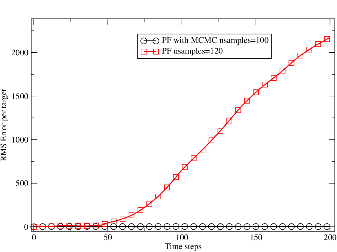
Figure 4 compares the effective sample size for the generic particle filter and the MCMC particle filter. Because the number of samples is different for the two filters we have plotted the effective sample size as a percentage of the number of samples. We have to note that, after about 50 steps, the generic particle filter started producing observation weights (before the normalization) which were numerically zero. This makes the normalization impossible. In order to allow the generic particle filter to continue we chose at random one of the samples, since all of them are equally bad, and assigned all the weight to this sample. We did that for all the steps for which the observation weights were zero before the normalization. As a result, the effective sample size for the generic particle filter drops down to 1 sample after about 50 steps. Once the generic particle filter deviates from the true target tracks there is no mechanism to correct it. Also, we tried assigning equal weights to all the samples when the observation weights dropped to zero. This did not improve the generic particle’s performance either. On the other hand, the MCMC particle filter maintains an effective sample size which is about $25\%$ of the number of samples.

3.3 Nonlinear observations

We continue with results for the nonlinear observation model (14). Figures 5 and 6 show the evolution in the $xy$ space of the true targets, the observations as well as the estimates of the MCMC particle filter. Again, as in the case of the linear observation model, the MCMC particle filter follows accurately the targets and there is no ambiguity in the identification of the target tracks.

The case of the nonlinear observation model is much more difficult than the case of the linear observation model. The reason is that for the nonlinear observation model, the observation errors, though constant in bearing and range space, they become position dependent in $xy$ space. In particular, when $x$ and/or $y$ are large, the observation errors can become rather large. This is easy to see by Taylor expanding the nonlinear transformation from bearing and range space to $xy$ space around the true target values. Suppose that the true target bearing and range are $\theta_{0},r_{0}$ and its $xy$ space position is $x_{0}=r_{0}\cos\theta_{0},y_{0}=r_{0}\sin\theta_{0}.$ Also, assume that the observation error in bearing and range space is, respectively, $\delta\theta$ and $\delta r.$ The $xy$ position of a target that is perturbed by $\delta\theta$ and $\delta r$ in bearing and range space is (to first order)

	$\displaystyle x$	$\displaystyle=x_{0}-y_{0}\delta\theta-\delta r\cos\theta_{0}$
	$\displaystyle y$	$\displaystyle=y_{0}+x_{0}\delta\theta-\delta r\sin\theta_{0}.$

Thus, the perturbation in $xy$ space can be significant even if $\delta\theta$ and $\delta r$ are small. In our example we have $\sigma_{\theta}=10^{-2}.$ So, when the true target $x$ and $y$ values become of the order of $10^{3}$ as happens for some of the targets, the observation value in bearing and range space can be quite misleading as far as the $xy$ space position of the target is concerned. As a result, even if one does a good job in following the observation in bearing and range space, the conditional expectation estimate of the $xy$ space position can be inaccurate.

With this in mind, we have used 200 samples for the MCMC particle filter and 220 samples for the generic particle filter. Again, the extra samples used for the generic particle filter more than account for the computational overhead of the MCMC particle filter. The performance of the MCMC particle filter is compared to the performance of the generic particle filter in Figure 7 by monitoring the evolution in time of the RMS error per target. The generic particle filter’s accuracy again deteriorates rather quickly. The error for the MCMC particle filter is larger than in the linear observation model but never exceeds about 80 even after 200 steps when the targets have reached large values of $x$ and/or $y.$ The average value of the RMS error over the entire time interval of tracking is about 22 with standard deviation of about 21. For the generic particle filter, the average of the RMS error over the time interval of tracking is about 760 with standard deviation of about 770.

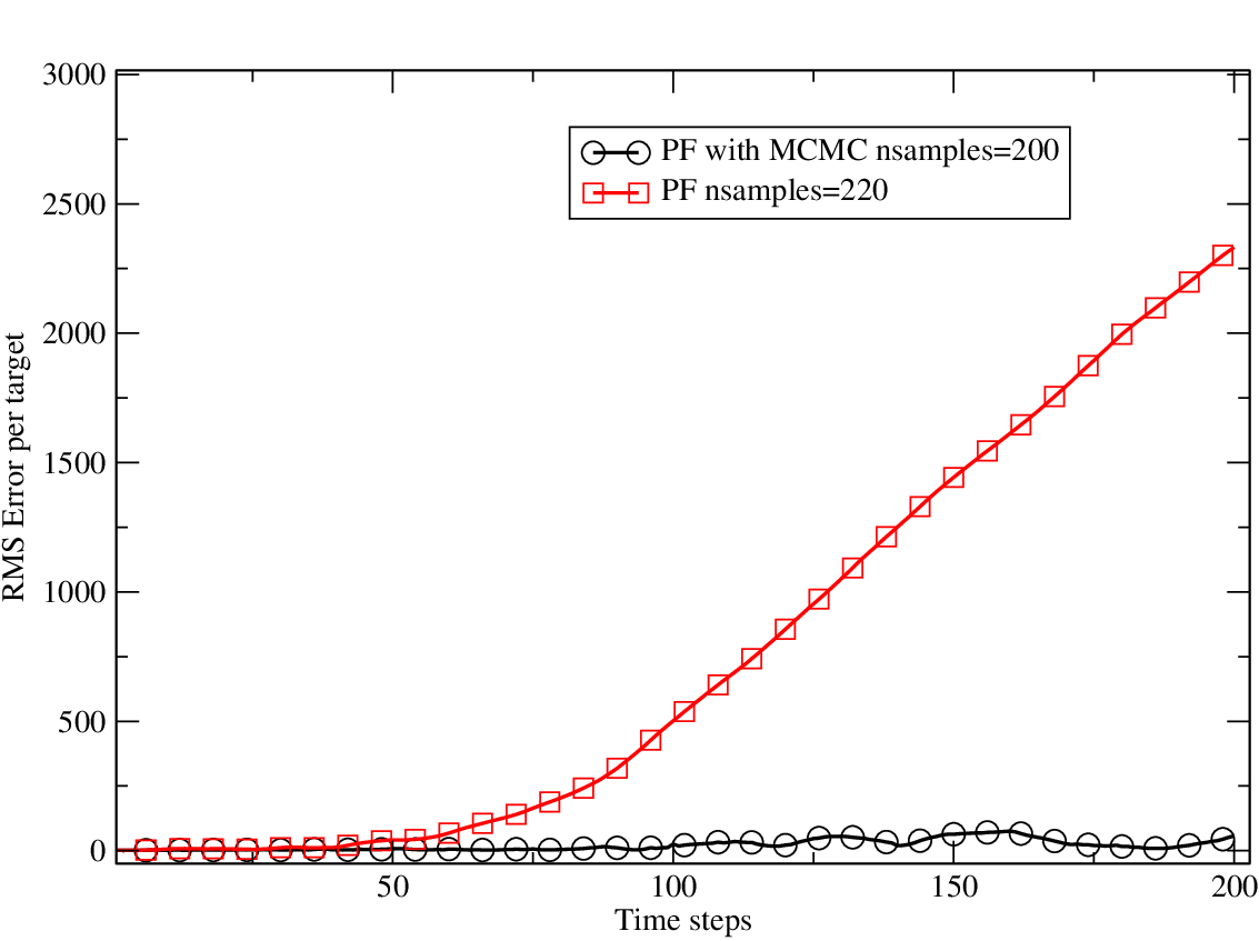
Figure 8 compares the effective sample size for the generic particle filter and the MCMC particle filter. After about 60 steps, the generic particle filter, started producing observation weights (before the normalization) which were numerically zero. This makes the normalization impossible. In order to allow the generic particle filter to continue we chose at random one of the samples, since all of them are equally bad, and assigned all the weight to this sample. We did that for all the steps for which the observation weights were zero before the normalization. As a result, the effective sample size for the generic particle filter drops down to 1 sample after about 60 steps. Once the generic particle filter deviates from the true target tracks there is no mechanism to correct it. Also, we tried assigning equal weights to all the samples when the observation weights dropped to zero. This did not improve the generic particle’s performance either. On the other hand, the MCMC particle filter maintains an effective sample size which is about $25\%$ of the number of samples.

4 Discussion

We have presented an algorithm for multi-target tracking which is based on drift homotopy for stochastic differential equations. The algorithm builds on the existing particle filter methodology for multi-target tracking by appending an MCMC step after the particle filter resampling step. The purpose of the addition of the MCMC step is to bring the samples closer to the observation. Even though the addition of an MCMC step for a particle filter has been proposed and used before [7], to the best of our knowledge, the use of drift homotopy to effect the MCMC step is novel (see also [16]).

We have tested the performance of the algorithm on the problem of tracking multiple targets evolving under the near constant velocity model [1]. We have examined two cases of observation models: i) a linear observations model involving the positions of the targets and ii) a nonlinear observation model involving the bearing and range of the targets. For both cases the proposed MCMC particle filter exhibited a significantly better performance than the generic particle filter. Since the MCMC particle filter requires more computations than the generic particle filter it is bound to be more expensive. However, the computational overhead of the MCMC particle filter is rather small, of the order of a few extra samples worth for the generic particle filter.

We plan to perform a detailed study of the proposed algorithm in more realistic cases involving clutter, spawning and merging of targets. Also, we want to study the behavior of the algorithm for cases with random birth and death events as well as for larger number of targets. Finally, the algorithm can be coupled to any target detection algorithm (see e.g. [14]) to perform joint detection and tracking.

Acknowledgements

We are grateful to Prof. J. Weare for many discussions and moral support. Also, we would like to thank the Institute for Mathematics and its Applications in the University of Minnesota for its support.

References

[1] Bar-Shalom Y. and Fortmann T.E., Tracking and Data Association, Academic Press, 1988.
[2] Bar-Shalom Y. and Blair W.D., Eds. Multitarget-Multisensor Tracking: Applications and Advances, vol. III, Norwood, MA, Artech House, 2000.
[3] Blackman S. and Popoli R., Design and Analysis of Modern Tracking Systems, Norwood, MA, Artech House, 1999.
[4] Chorin, A.J. and Tu X., Implicit sampling for particle filters, Proc. Nat. Acad. Sc. USA 106 (2009) pp. 17249-17254.
[5] Doucet A., de Freitas N. and Gordon N. (eds.) , Sequential Monte Carlo Methods in Practice, Springer NY, 2001.
[6] Fortmann T. E., Bar-Shalom Y. and Scheffe M., Sonar tracking of multiple targets using joint probabilistic data association, IEEE J. Ocea. Eng., vol.8 (1983) pp.173-184.
[7] Gilks W. and Berzuini C., Following a moving target. Monte Carlo inference for dynamic Bayesian models, J. Royal Stat. Soc. B 63 (1) (1999) pp. 2124-2137.
[8] Gordon N.J., Salmond D.J. and Smith A.F.M., Novel approach to nonlinear/non-Gaussian Bayesian state estimation, Proc. Inst. Elect. Eng. F 140(2) (1993) pp. 107-113.
[9] Liu J.S., Monte Carlo Strategies in Scientific Computing, Springer NY, 2001.
[10] Liu J.S. and Chen R. Sequential Monte Carlo Methods for Dynamic Systems. Journal of the American Statistical Association, vol.93 no. 443 (1993) pp. 1032-1044.
[11] Mahler R. P., Statistical Multisource-Multitarget Information Fusion, Artech House Publishers MA, 2007.
[12] Mahler R. P. S., Multitarget Bayes filtering via first-order multitarget moments, IEEE Trans. Aero. Elect. Sys., Vol. 39 no. 4 (2003) pp. 1152-1178.
[13] Mahler R.P.S. and Maroulas V. Tracking Spawning Objects, (2010) submitted.
[14] Ng W., Li J.F., Godsill S.J. and Vermaak J., A hybrid approach for online joint detection and tracking for multiple targets, Proc. IEEE Aerospace Conference (2005) pp. 2126-2141.
[15] Snyder C., Bengtsson T., Bickel P. and Anderson J., Obstacles to High-dimensional Particle Filtering, Mon. Wea. Rev., Vol. 136 (2008) pp. 4629-4640.
[16] Stinis P., Conditional path sampling for stochastic differential equations by drift homotopy, (2010), arXiv:1006.2492v1.
[17] Stoer J, and Bulirsch R., Introduction to Numerical Analysis, Third Edition, Springer 2002.
[18] Vermaak J., Godsill S. and Perez P., Monte Carlo filtering for multi-target tracking and data association, IEEE Trans. Aero. Elect. Sys., 41(1) (2005) pp. 309-332.
[19] Vo B-N., Singh S. and Doucet A., Sequential Monte Carlo Methods for Multi-Target Filtering with Random Finite Sets, IEEE Trans. Aero. Elect. Sys., 41(4) (2005) pp. 1224-1245.
[20] Weare J., Particle filtering with path sampling and an application to a bimodal ocean current model, J. Comp. Phys. 228 (2009) pp. 4312-4331.

	$\displaystyle p(X_{T_{k}}\|\{Z_{T_{j}}\}^{k}_{j=1})$	$\displaystyle\propto g(X_{T_{k}},Z_{T_{k}})p(X_{T_{k}}\|\{Z_{T_{j}}\}^{k-1}_{j=1}),$		(2)
	$\displaystyle\text{where}\;\;p(X_{T_{k}}\|\{Z_{T_{j}}\}^{k-1}_{j=1})$	$\displaystyle=\int p(X_{T_{k}}\|X_{T_{k-1}})p(X_{T_{k-1}}\|\{Z_{T_{j}}\}^{k-1}_{j=1})dX_{T_{k-1}}.$		(3)