Grid diagrams of Lorenz links

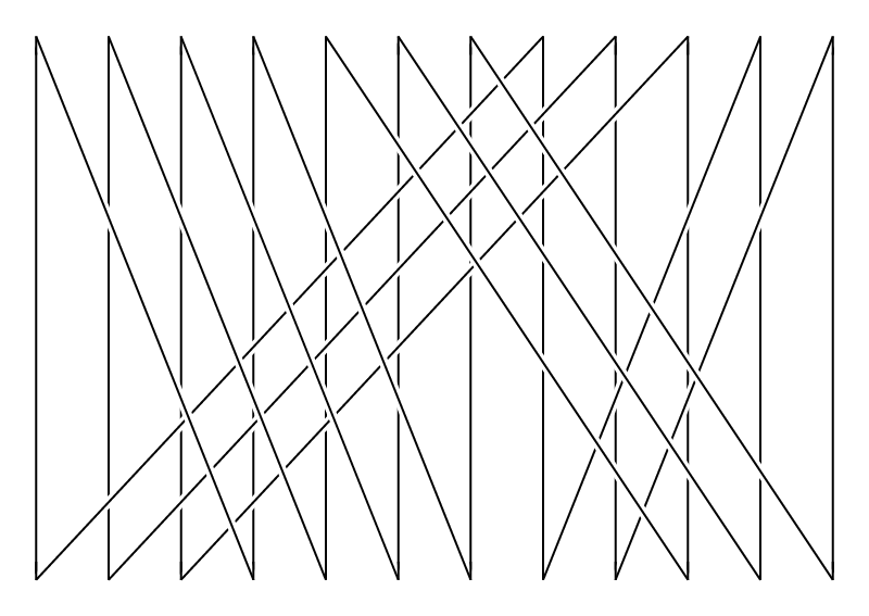
Lorenz links are periodic orbits of the Lorenz ”strange attractor”, which arises in physics. See [3] for details. Twisted links are a generalization of torus links: it is allowed to twist not the whole set of strings but also some of its subsets. We will introduce a class of oriented links by putting restrictions on their grid diagrams and then we will show that it coincides with the class of Lorenz links and with that of twisted links.

Definition 1. A permutation $\sigma\in S_{n}$ is called a shuffle if there exists k such that:

Let $\sigma$ be a shuffle such that $\sigma(i)\neq i$ for all $i=1,...,n$. Then the closure of the permutation braid associated to the shuffle $\sigma$ is called a Lorenz link. Lorenz links inherit their orientation from the corresponding braids. We will associate the following vector to $\sigma$

and call it the Lorenz vector of $\sigma$.

We will denote the Lorenz link corresponding to $\sigma$ by the associated Lorenz vector. We will also use the following short notation for this vector:

Example 1. In Fig.1 the Lorenz link with Lorenz vector $\langle 3^{4},5^{3}\rangle$ is shown.

Definition 2. Twisted links (T-links) are the closures of braids on n strings of the following form:

The T-link, associated to this braid is denoted by T(($p_{1},q_{1}$),…,($p_{s},q_{s}$)) (see Fig.2). The class of T-links is a generalization of the class of torus links, which corresponds to $s=1$. T-links also inherit their orientations from the braids.

Example 2. In Fig.2 the T-link T((3,4),(5,3)) is shown.

Definition 3. Let $\sigma\in S_{n}$ be a shuffle and $v$ is its Lorenz vector. We will denote by diag($v$) (or by diag($\sigma$)) the following link given by the coordinates of the vertices of its grid presentation (see [2] for the definition of grid (rectangular) presentations):

If $\sigma(i)>i$ a vertical edge with x-coordinate i is oriented upwards; otherwise it is oriented downwards. Horizontal edges are oriented appropriately. We will call such links diagonal.

Example 3. In Fig.3 the diagonal link diag($\langle 3,3,3,3,5,5,5\rangle$) is shown.

Theorem 1. The class of diagonal links coincides with the class of Lorenz links. More precisely, the diagonal link diag($\langle{p_{1}}^{q_{1}},{p_{2}}^{q_{2}},...,{p_{s}}^{q_{s}}\rangle$) is isotopic to the Lorenz link $\langle{p_{1}}^{q_{1}},{p_{2}}^{q_{2}},...,{p_{s}}^{q_{s}}\rangle$.

Proof. Let’s denote the diagonal $x=y$ of diag($\langle{p_{1}}^{q_{1}},{p_{2}}^{q_{2}},...,{p_{s}}^{q_{s}}\rangle$) by $l$. Let’s denote the set of vertical edges with x-coordinate less or equal to $q_{1}+q_{2}+...+q_{s}$ by $L$. The remaining vertical edges will form the set $R$.

Now we introduce the isotopy. First we rotate our grid diagram by $45^{0}$ clockwise. Next we rotate each edge from $L$ by $45^{0}$ counterclockwise around its lower end and stretch them as necessary so as to have all their upper ends on a straight line parallel to $l$. Then we will apply the same procedure to $R$, rotating the edges around their upper ends. The other edges, which were horizontal before the rotation are adjusted appropriately. Refer to Fig.4 for an example.

Next we fold our link along the horizontal line $l$ and put the lower part over the upper one. Now there are only two rows of vertices of our piecewise-linear planar diagram. There are three layers of edges: the middle layer consists of $q_{1}+q_{2}+...+q_{s}+p_{s}$ vertical edges, the top layer consists of $p_{s}$ edges crossing the edges from the middle layer negatively, the bottom layer consists of $q_{1}+q_{2}+...+q_{s}$ edges crossing the edges from the middle layer negatively. Consider the edges of the bottom layer. They don’t cross each other, so there will be no obstruction to pull them aside and place in the top layer. Refer to Fig.1 for an example. This is a closed permutation braid associated to $\sigma$, which is a shuffle. Thus it is the Lorenz link $\langle{p_{1}}^{q_{1}},...,{p_{s}}^{q_{s}}\rangle$.

Theorem 2. The class of diagonal links coincides to the class of twisted links. Precisely, the diagonal link diag($\langle{p_{1}}^{q_{1}},{p_{2}}^{q_{2}},...,{p_{s}}^{q_{s}}\rangle$) is isotopic to the twisted link $T((p_{1},q_{1}),...,(p_{s},q_{s}))$.

Proof. Let’s cut open the horizontal edges of diag($\langle{p_{1}}^{q_{1}},{p_{2}}^{q_{2}},...,{p_{s}}^{q_{s}}\rangle$) with y-coordinate $\sigma(i)$ $(i>q_{1}+q_{2}+...+q_{s})$ and connect them ”through the infinity”. Refer to Fig.5 for an example.

This is a diagram of a braid on $p_{s}$ strings, oriented rightwards. The strings are numbered bottom-to-up. All crossings are placed over the former diagonal of the diagonal link. They are induced by the vertical edges of the diagonal link with x-coordinate $i\leq q_{1}+q_{2}+...+q_{s}$. Each such edge contributes $\sigma_{1}\sigma_{2}...\sigma_{\sigma(i)-1}$ to the braid word since the left string crosses over the next $\sigma(i)-1$ strings. Finally we get the following braid word:

Thus we got T(($p_{1},q_{1}$),…,($p_{s},q_{s}$)).

Corollary([1]).The class of Lorenz links coincides to the class of twisted links. Precisely, the Lorenz link $\langle{p_{1}}^{q_{1}},{p_{2}}^{q_{2}},...,{p_{s}}^{q_{s}}\rangle$ is isotopic to the twisted link T(($p_{1},q_{1}$),…,($p_{s},q_{s}$)).

References

- [1] Joan Birman, Ilya Kofman. A new twist on Lorenz links. Journal of Topology 2(2009), 227-248.
- [2] Ivan Dynnikov. Arc-presentations of links. Monotonic simplification. Fund. Math. 190 (2006), 29-76.
- [3] J.Birman, R.Williams: Knotted periodic orbits in dynamical systems. I. Lorenz’s equations. Topology 22(1983), no.1, 47–82.