Thrust at N3LL with Power Corrections and a Precision Global Fit for
Abstract
We give a factorization formula for the thrust distribution with based on soft-collinear effective theory. The result is applicable for all , i.e. in the peak, tail, and far-tail regions. The formula includes fixed-order QCD results, resummation of singular partonic terms with N3LL accuracy, hadronization effects from fitting a universal nonperturbative soft function defined in field theory, bottom quark mass effects, QED corrections, and the dominant top mass dependent terms from the axial anomaly. We do not rely on Monte Carlo generators to determine nonperturbative effects since they are not compatible with higher order perturbative analyses. Instead our treatment is based on fitting nonperturbative matrix elements in field theory, which are moments of a nonperturbative soft function. We present a global analysis of all available thrust data measured at center-of-mass energies to GeV in the tail region, where a two parameter fit to and the first moment suffices. We use a short distance scheme to define , called the R-gap scheme, thus ensuring that the perturbative does not suffer from an renormalon ambiguity. We find , with , where the displayed -sigma errors are the total experimental error, the hadronization uncertainty, and the perturbative theory uncertainty, respectively. The hadronization uncertainty in is significantly decreased compared to earlier analyses by our two parameter fit, which determines with 16% uncertainty.
I Introduction
A traditional method for testing the theory of strong interactions (QCD) at high-precision is the analysis of jet cross sections at colliders. Event shape distributions play a special role as they have been extensively measured with small experimental uncertainties at LEP and earlier colliders, and are theoretically clean and accessible to high-order perturbative computations. They have been frequently used to make precise determinations of the strong coupling , see e.g. Ref. [1] for a review. One of the most frequently studied event shape variables is thrust [2],
| (1) |
where the sum is over all final-state hadrons with momenta . The unit vector that maximizes the right-hand side (RHS) of Eq. (1) defines the thrust axis. We will use the more convenient variable . For the production of a pair of massless quarks at tree level , so the measured distribution for involves gluon radiation and is sensitive to the value of . The thrust value of an event measures how much it resembles two jets. For values close to zero the event has two narrow, pencil-like, back-to-back jets, carrying about half the center-of-mass (c.m.) energy into each of the two hemispheres defined by the plane orthogonal to . For close to the multijet endpoint , the event has an isotropic multi-particle final state containing a large number of low-energy jets.
On the theoretical side, for the dynamics is governed by three different scales. The hard scale is set by the c.m. energy . The jet scale, is the typical momentum transverse to of the particles within each of the two hemispheres, or the jet invariant mass scale if all energetic particles in a hemisphere are grouped into a jet. There is also uniform soft radiation with energy , called the soft scale. The physical description of the thrust distribution can be divided into three regions,
| peak region: | ||||||
| tail region: | (2) | |||||
| far-tail region: |
In the peak region the hard, jet, and soft scales are , , and , and the distribution shows a strongly peaked maximum. Theoretically, since one needs to sum large (double) logarithms, , and account for the fact that , so is affected at leading order by a nonperturbative distribution. We call this distribution the nonperturbative soft function. The tail region is populated predominantly by broader dijets and 3-jet events. Here the three scales are still well separated and one still needs to sum logarithms, but now , so soft radiation can be described by perturbation theory and a series of power correction parameters . Finally, the far-tail region is populated by multijet events. Here the distinction of the three scales becomes meaningless, and accurate predictions can be made with fixed-order perturbation theory supplemented with power corrections. The transition to this region must be handled carefully since including a summation of terms in this region spoils the cancellations that take place at fixed order multijet thresholds, and hence would induce uncertainties that are significantly larger than those of the fixed-order results.
Recently two very important achievements were made improving the theoretical description of event shape distributions in annihilation. First, in the work of Gehrmann et al. in Refs. [3, 4] and Weinzierl in Refs. [5, 6] the full set of contributions to the 2-, 3- and 4-jet final states were determined. These results were made available in the program package EERAD3 [3]. Second, soft-collinear effective theory (SCET) [7, 8, 9, 10, 11] provides a systematic framework to treat nonperturbative corrections [12, 13] and to factorize and compute hard, collinear and soft contributions for jet production to all orders in [14, 15, 16], building on earlier all orders QCD factorization results [17, 18, 19]. The SCET framework allows for the summation of large logarithms at higher orders, as demonstrated by the analytic calculation of the thrust distribution at N3LL order by Becher and Schwartz in Ref. [20].11 1 The calculation of Ref. [20] also revealed a numerical problem at small in the initial fixed-order results of Refs. [3, 4]. In contrast, the classic exponentiation techniques of Ref. [21] for event shapes have so far only been carried out to NLL order. Also, the anomalous dimensions in SCET relevant for thrust are valid over perturbative momentum scales, and there are no Landau pole ambiguities in the resummation at any order. In addition, as we will discuss in the body of our paper, SCET provides a rigorous framework for including perturbative and nonperturbative contributions, which can be used to connect power corrections in factorization theorems to those in an operator expansion for thrust moments. Moreover it provides a simple method to simultaneously treat the peak, tail, and far-tail regions.
Several determinations of in the tail region have been carried out incorporating the fixed-order results, which we have collected in Tab. 1.
| sum logs | power corrections | ||
|---|---|---|---|
| Ref. [22] | no | Monte Carlo (MC) | |
| Ref. [20] | N3LL | uncertainty from MC | |
| Ref. [23] | NLL | effective coupling | |
| model | |||
| Ref. [24] | NLL | Monte Carlo | |
| Ref. [25] | NLL | Monte Carlo |
They differ on which event shape data has been used for the fits, on the accuracy of the partonic resummation of logarithms in the theory formula, the approach for nonperturbative hadronization effects, and how the theory errors are estimated. It is instructive to compare the analyses by Dissertori et al. [22, 25] and by Becher and Schwartz [20], which both used the error band method [26] to determine theoretical uncertainties. The improved convergence and reduced theoretical uncertainty for obtained by Becher and Schwartz indicates that the summation of logarithms beyond NLL order level is important. Both the analyses by Dissertori et al. and Becher and Schwartz are limited by the fact that they used Monte Carlo (MC) generators to estimate the size of nonperturbative corrections.
The use of MC generators to estimate power corrections is problematic since the partonic contributions are based on LL parton showers with at most one-loop matrix elements, complemented by hadronization models below the shower cutoff that are not derived from QCD. The parameters of these models have been tuned to LEP data, and thus unavoidably encode both nonperturbative effects as well as higher order perturbative corrections. Hence, one must worry about double counting, and this makes MC generators unreliable for estimating nonperturbative corrections in higher order LEP analyses. Moreover, purely perturbative results for event shapes in the scheme such as those in Refs. [22, 20, 25, 6] suffer from infrared effects known as infrared renormalons (see Ref. [27] for a review of the early literature). These infrared effects arise because fluctuations from large angle soft radiation down to arbitrarily small momenta are included in the perturbative series and can cause unphysical large corrections already in low-order perturbative QCD results. On the other hand, the hard shower cutoff protects the parton level MC from infrared renormalons. Hence one cannot rigorously combine MC hadronization effects with strict perturbative results. From the two points raised above, we conclude that the results obtained in Refs. [22, 20, 25] contain a systematic theoretical error from nonperturbative effects that can be quite sizeable. We emphasize that this criticism also applies in part to the numerous earlier event shape analyses which estimated nonperturbative corrections using MC generators, see Ref. [1] for a review.
The presence of power corrections in have been discussed in earlier literature [28, 29, 30, 31, 32, 33, 34], where it has been argued that the leading effect is a shift in the thrust distribution, with . The analyses with the results, that discuss nonperturbative effects in the thrust tail region without relying on MC generators are: Ref. [20] which examined a power correction in a simple soft function model, but due to the large induced uncertainty on does not use it for their final error analysis, and Ref. [23] which uses the effective coupling model.
For the most accurate data at the change to the extracted from including the leading power correction can be quite significant, at the 10% level. We can derive this estimate by a simple calculation. We first write the cross section with a shift due to the power correction, . Assuming is proportional to , and expanding for , one can easily derive that the change in the value extracted from data due to the existence of the power correction is
| (3) |
The expression in Eq. (3) gives a scaling estimate for the fractional change in from an analysis with the power correction compared to one without, using data at . To the extent that the assumptions stated above are realized, the slope factor should be constant. In Fig. 1 we show the slope factor computed from experimental data at . The figure shows that the slope factor is indeed only weakly depending on in the tail region and we get . The remaining visible variation in is related to subleading nonperturbative and higher power effects that are not accounted for in our simple scaling estimate. For a QCD power correction of natural size, , Eq. (3) gives for . The magnitude of this effect makes it important to treat power corrections as accurately as possible in a fit to thrust data. We will show in later sections of this work that the relative downward shift in the fitted due to nonperturbative effects is indeed at the level of the scaling estimate of .

In the NLL/ analysis by Davison and Webber [23] the nonperturbative effects are incorporated through a power correction which is fit together with to the experimental data. The power correction is formulated from the low-scale effective coupling model of Ref. [35], which modifies below GeV, and defines as the average value of the coupling between and . It is important that the effective coupling model correctly predicts the dependence of the leading nonperturbative power correction in factorization [35, 18]. This model also induces a subtraction of perturbative contributions below the momentum cutoff (based on the running coupling approximation) and thus removes infrared renormalon ambiguities.22 2 Another thrust analysis where infrared renormalon contributions have been removed from the partonic contributions is by Gardi and Rathsman in Refs. [36, 37], which used a principal value prescription for the inverse Borel transformation of the thrust distribution. Their analysis was prior to the new fixed-order computations, and hence was not included in Table 1. However the model is not based on factorization, and hence this treatment of nonperturbative corrections is not systematically improvable. It is therefore not easy to judge the corresponding uncertainty. Another problem of the effective coupling model is that its subtractions involve large logs, , which are not resummed. This effects the dependence in the interplay between perturbative and nonperturbative effects.
In this paper we extend the event shape formalism to resolve the theoretical difficulties mentioned above. Our results are formulated in the SCET framework, and hence are rigorous predictions of QCD. The formula we derive has a N3LL order summation of logarithms for the partonic singular terms, and fixed-order contributions for the partonic nonsingular terms. Our theoretical improvements beyond earlier work include:
- •
A factorization formula that can be simultaneously applied to data in the peak and the tail regions of the thrust distribution and for multiple c.m. energies , as well as being consistent with the multijet thresholds in the far-tail region.
- •
In the factorization formula a nonperturbative soft function defined from field theory is implemented using the method of Ref. [16] to incorporate hadronization effects. To achieve independence of a particular analytic ansatz in the peak region, the nonperturbative part of the soft function uses a linear combination of orthogonal basis functions that converge quickly for confined functions [38].
- •
In the tail region the leading power correction to is determined by a nonperturbative parameter that appears through a factorization theorem for the singular distribution. is a field theory matrix element of an operator, and is also related to the first moment of the nonperturbative soft function. In the tail region the effects of hadronization corrections are included for the nonsingular corrections that are kinematically subleading in the dijet limit, based on theoretical consistency with the far-tail region.
- •
Defining the matrix element in , the perturbative cross section suffer from an renormalon. In our analysis this renormalon is removed by using an R-gap scheme for the definition of [16]. This scheme choice induces subtractions on the leading power cross section which simultaneously remove the renormalon there. Large logarithms in the subtractions are summed to all orders in using R-evolution equations given in Refs. [39, 40].
- •
- •
QED corrections at NNLL order are incorporated, counting . This includes QED Sudakov effects, final state radiation, and QED/QCD renormalization group interference.
- •
The 3-loop finite term of the quark form factor in is extracted using the results of Ref. [42], and is included in our analysis.
- •
The most important corrections from the axial anomaly are included. The anomaly modifies the axial-vector current contributions at by terms involving the top quark mass.
Electroweak effects from virtual and loops mostly effect the normalization of the cross section and so their dominant contribution drops out of [43, 44]. These corrections are not included in our analysis.
For the numerical analyses carried out in this work we have created within our collaboration two completely independent codes. One code within Mathematica [45] implements the theoretical expressions exactly as given in this paper, and one code is based on theoretical formulae in Fourier space and realized as a fast Fortran code suitable for parallelized runs on computer clusters. These two codes agree for the thrust distribution at the level of .
While the resulting theoretical code can be used for all values of , in this paper we focus our numerical analysis on a global fit of thrust data in the tail region, for c.m. energies between and GeV, to determine .33 3 Throughout this paper we use the scheme for with five light flavors. Our global fit exhibits consistency across all available data sets, and reduces the overall experimental uncertainty. For a single we find a strong correlation between the effect of and on the cross section. This degeneracy is broken by fitting data at multiple s. The hadronization uncertainty is significantly decreased by our simultaneous global fit to and . To estimate the perturbative uncertainty in the fit we use a random scan in a 12-dimensional theory parameter space. This space includes 6 parameters for -variation, 3 parameters for theory uncertainties related to the finite statistics of the numerical fixed-order results, one parameter for the unknown 4-loop cusp anomalous dimension, and two parameters for unknown constants in the perturbative 3-loop jet and 3-loop soft functions. The scan yields a more conservative theory error than the error band method [26]. Despite this we are able to achieve smaller perturbative uncertainties than earlier analyses due to our removal of the renormalon and the inclusion of . We also analyze in detail the dependence of the fit results on the range in used in the fit.
The outline of the paper is as follows. In Sec. II we introduce the theoretical framework and discuss the various theoretical ingredients in our final formula. In Sec. III we present the profile functions which allow us to simultaneously treat multiple regions, and discuss the 6 parameters used for -variation in the analysis of the perturbative uncertainty. In Sec. IV we review the parametrization of the nonperturbative function. In Sec. V we discuss the normalization of our distributions and compare results at different orders in perturbation theory for: fixed-order results, adding the log resummation, adding the nonperturbative corrections, and adding the renormalon subtractions. In Sec. VI we discuss the experimental data and the fit procedure. Our results for and the soft function moment from the global fit are presented in Sec. VII, including a discussion of the theory errors. In Sec. VIII we use our tail fit results to make predictions in the far-tail and peak regions, and compare with data. Cross checks on our code are discussed in Sec. IX, including using it to reproduce the earlier lower precision fits of Dissertori et al. [22] and Becher and Schwartz [20]. Section X contains our conclusions and outlook, including prospects for future improvements based on the universality of the parameter . The analytic theoretical expressions that went into our analysis for massless quarks and QCD effects are presented in condensed form in Appendix A. In Appendix B we use the operator product expansion for the soft function in the tail region, discussing uniqueness and deriving an all order relation for the Wilson coefficient of . In Appendix C we use an OPE for the first moment of the thrust distribution to show that it involves the same at lowest order. Readers most interested in our numerical results can skip directly to Sections VI and VII.
II Formalism
II.1 Overview
The factorization formula we use for the fits to the experimental thrust data is
| (4) |
Here contains the singular partonic QCD corrections and with the standard plus-functions as defined in Eq. (95). It also contains the singular partonic QED corrections depending on which are discussed in Sec. II.8. This term accounts for matrix element corrections and the resummation of terms within the SCET formalism up to N3LL order, which we discuss in Sec. II.3. Our definition of N3LL, N3LL′, and other orders is discussed in detail in Sec. II.2 (see also Tab. 2).
The term , which we call the nonsingular partonic distribution, contains the thrust distribution in strict fixed-order expansion with the singular terms subtracted to avoid double counting. The most singular terms in scale as for .44 4 For the resummation of terms is currently unknown. These terms could be determined with subleading factorization theorems in SCET. Our implementation of nonsingular terms is discussed in detail in Sec. II.5.
Finally, contains corrections to the singular and nonsingular cross sections due to the finite mass of the bottom quark. The -mass corrections are implemented as a difference of the massive and massless cross sections computed at NNLL order as discussed in Sec. II.7.
The function that is convoluted with these partonic cross sections in Eq. (4) describes the nonperturbative effects from soft gluons including large angle soft radiation [18, 46]. The definition of also depends on the hemisphere prescription inherent to the thrust variable. This is a hadronic function that enters in a universal way for both massless and massive cross sections, and is independent of the value of . The universality of in Eq. (4) follows from the leading power thrust factorization theorem [18, 14, 15], and the thrust factorization theorem for massive quarks in Refs. [14, 41]. Our treatment of the convolution of with yields a consistent treatment of multijet thresholds and the leading power correction to the operator expansion for the first moment of thrust. Details of our implementation of power corrections and nonperturbative corrections are discussed in Sec. II.4 and Sec IV. The function is normalized to unity and can be determined from experimental data. Its form depends on a gap parameter and additional moment parameters which are discussed below.
The factorization formula given in Eq. (4) can be applied simultaneously in the peak, tail, and the far-tail regions of Eq. (2), i.e. for all values. In the peak region is significantly smaller than , and the full analytic form of the soft nonperturbative function is relevant to determine the -distribution since . Because , the summation of logarithms of is also crucial to achieve an accurate theoretical description.
For much of the tail region the summation of terms remains important, although this is no longer the case when we reach . Likewise, the dominance of the singular partonic contributions remains as long as , but the nonsingular terms become more important for increasing (see Fig. 7 below). Near the nonsingular terms become equal in size to the singular terms with opposite sign. Since in the tail region the effects of can be parameterized in terms of the moments
| (5) |
where since is normalized. Their importance is determined by as discussed in Sec. II.4, so the first moment parameterizes the dominant power correction and higher moments provide increasingly smaller corrections. The first moment is defined by
| (6) |
where , is similar but in the representation, and we trace over color. Here
| (7) |
is a derivative operator55 5 Note that is defined in the c.m. frame of the colliding . One may also write where measures the sum of absolute transverse momenta at a given rapidity with respect to the thrust axis [18, 47]. involving light-like vectors and . is the field theory analog of the parameter employed in the low-scale effective coupling approach to power corrections. Since the renormalon subtractions depend on a cutoff scale and the renormalization scale , all moments as well as are scale and scheme dependent quantities. The scheme we use to define is described in Sec. II.6. In our fit to experimental data we use the R-gap scheme, and extract the first moment at a reference scale GeV, i.e. we use and hence . In the factorization theorem the gap appears evaluated at and the scales () are connected to the reference scales () using renormalization group equations.
Finally, in the far-tail region the singular and the nonsingular partonic contributions and become nearly equal with opposite signs, exhibiting a strong cancellation. This is due to the strong suppression of the fixed-order distribution in the three- and four-jet endpoint regions at in fixed-order perturbation theory. In this region the summation of logarithms of must be switched off to avoid messing up this cancellation. Here our Eq. (4) reduces to the pure fixed-order partonic thrust distribution supplemented with power corrections coming from the convolution with the soft function. All three regions are smoothly joined together in Eq. (4). The proper summation (or non-summation) of logarithms is achieved through -dependent renormalization scales, , , and which we call profile functions. They are discussed in detail in Sec. III.
In the following subsections various ingredients of the factorization formula of Eq. (4) are presented in more detail. Compact results for the corresponding analytic expressions for massless quarks in QCD are given in App. A. In Secs. II.7 and II.8 we describe how finite bottom mass and QED corrections are included in our analysis. The full formulae for these corrections will be presented in a future publication.
II.2 Order Counting
a) Perturbative Corrections
b) Nonperturbative Corrections with
cusp
non-cusp
matching
nonsingular
LL
1
-
tree
1
-
-
-
NLL
2
1
tree
2
-
1
-
NNLL
3
2
1
3
1
2
1
N3LL
3
2
4
2
3
2
NLL′
2
1
1
2
1
1
1
NNLL′
3
2
2
3
2
2
2
N3LL′
3
3
4
3
3
3
peak (any )
tail and far-tail ()
p.c.
In the classic order counting used for fits to event shape distributions it is common to separately quote orders for the summation of logarithms and the fixed-order matching contributions. For fixed-order contributions the contributions are called LO, the contributions are called NLO, etc. This counting is motivated from the fact that at tree level the fixed-order thrust distribution vanishes for . For the summation one refers to LL (leading-log) summation if the one-loop cusp anomalous dimension is used to sum the double Sudakov logs, and NLL (next-to-leading-log) if the two-loop cusp and the one-loop non-cusp anomalous dimension terms are also included.
In our analysis the summation orders (LL, NLL, …) match the classical language. For the fixed-order contributions we account for the tree level in LL and NLL, and we include corrections at NLL′ and NNLL, etc, as shown in Tab. 2a. In SCET the summation can be carried out at both NNLL and N3LL [20]. The corresponding loop orders for the anomalous dimensions are also shown in Tab. 2a. Within SCET the summation of logarithms is achieved by renormalization group evolution and the fixed-order corrections enter as series evaluated at each of the transition scales , , and which we refer to as matching or matrix element corrections. The logs in the singular thrust cross section exponentiate to all orders if we use , the Fourier-transformed variable to . The orders we consider correspond to summing the terms
| (8) | ||||
where , and the series in the exponent makes clear the structure of the large logs that are summed at each order.
The nonsingular counting in Tab. 2a for the fixed-order series in must be the same as for the matching and matrix element corrections to ensure that we exactly reproduce the fixed-order cross section when the resummed result is expanded. Since the relative importance of the log resummation and the nonsingular terms varies depending on the -region, we also consider an alternative “primed” counting scheme. In the primed counting all series for fixed-order quantities are included to one higher order in . In this counting scheme the fixed-order results occur in N3LL′, which is the order we use for our final analysis.
Also shown in Tab. 2a are columns for the fixed-order gap subtractions , and the gap anomalous dimensions . These terms are required to remove the leading renormalon from the perturbative corrections, while still maintaining the same level of log resummation for terms in the cross section. The resummation of these large logarithms is missing in the recent analysis of Ref. [23] and is discussed further in Sec. II.6.
A crucial aspect of our analysis is the inclusion of power corrections in a rigorous manner through field theoretic techniques. In the effective theory there are several types of power corrections which arise from the possible ratios of the scales , , , and :
| (9) |
Any power correction can be taken as a cross-term between types 1) and 2) for the purpose of enumeration. The type 1 power corrections are enhanced by the presence of the soft scale and are encoded by the moments of the soft function. Type 2 are kinematic power corrections that occur because of the expansion about small , and can be computed with perturbation theory. The importance of these first two types depends on the region considered in Eq. (2), with all terms in type 2 becoming leading order for the far-tail region. Type 3 are non-enhanced power correction that are of the same size in any region. There are also cross-terms between the three types.
In our analysis we keep all power corrections of types 1 and 2, and the dominant terms of type 3. Our treatment of the nonsingular cross section also includes cross-terms between 1 and 2 in a manner that is discussed in Sec. II.4. For the different thrust regions we display the relevant terms kept in our analysis in Tab. 2b. The nonsingular cross section corrections fully account for the power corrections of type 2. The factor in the peak region denotes the fact that we sum over all type 1 power corrections from the leading soft function. In the tail and multijet regions we only consider the first three orders: k=0 (partonic result), k=1 (power correction involving ) and , k=2 (power correction involving ). Here terms are used in our error analysis for our simultaneous fit to and . The leading power correction that is not fully captured in all regions is of type 3, and are of . Since our analysis is dominated by or larger, parametrically this gives an uncertainty of
| (10) |
in our final fit (taking to obtain the number here). This estimate has been validated by running our fits in the presence of an additional power correction.66 6 To perform this test we include an correction in the normalized thrust cross section, vary , and perform our default fit to and as described in Sec. VI. This variation causes only a change to these fit parameters, which is smaller than the estimate in Eq. (10).
II.3 Singular Partonic Distribution
The singular partonic thrust distribution contains the most singular terms and that arise from perturbation theory. Using SCET one can derive a factorization theorem for these terms which allows for the resummation of the logarithmic terms to all orders in perturbation theory. In massless QCD the factorization formula for the perturbative corrections involving reads
| (11) |
Here is the total partonic cross section for quark pair production at tree level from a current of type as explained below. Large logs are summed by the renormalization group factors between the hard scale and , between the jet scale and , and between the soft scale and . The choice of is arbitrary and the dependence on cancels out exactly when working at any particular order in the resummed expansion. Short distance virtual corrections are contained in the hard function . The term is the thrust jet function. The term is the partonic soft function and the -dependent exponential implements the perturbative renormalon subtractions. There are four renormalization scales governing the factorization formula, the hard scale , the jet scale , the soft scale , and the renormalon subtraction scale . We have to properly sum logarithms related to the renormalon subtractions, and there is also a renormalization group evolution in . The typical values for , , and depend on as discussed in Sec. III.
The total tree level partonic cross section depends on the c.m. energy , the -mass, and -width, and has six types of components, , , , , , , where the first index denotes flavor, , , and , and the other index denotes production through the vector () and axial-vector () currents. For QCD corrections we have the hard functions , , , and , where the vector current terms do not depend on the flavor of the quark. For massless quark production the axial-vector hard functions differ from the vector due to flavor singlet contributions. All six ’s and ’s are relevant for the implementation of the -mass and QED corrections. Since we use data taken for energies close to the Z pole we adopt as the Z-boson propagator which is the form of the width term used for thrust data analyses. The modifications of Eq. (11) required to include QED effects are discussed in Sec. II.8.
The hard factor contains the hard QCD effects that arise from the matching of the two-jet current in SCET to full QCD. For we have , and the full hard function with dependence is given in Eq. (84). For the flavor nonsinglet contributions where the final-state quarks are directly produced by the current one can obtain the matching coefficient from the on-shell quark vector current form factor, which is known to [48, 49, 50, 51, 52, 42]. Converting the bare result in Ref. [52] (see also Refs. [42, 53]) to the scheme and subtracting divergences present in SCET graphs, the three-loop non-singlet constant, which is one of the new ingredients in our analysis, is
| (12) |
For we have , which is the value used for our analysis.77 7 The analytic expression for in Eq. (12) is consistent with Eq. (7.3) given in Ref. [54].
The axial-vector hard functions and are equal to up to additional singlet corrections that enter at and . The fact that the SCET hard functions have these singlet corrections was discussed in Ref. [55]. At only the axial-vector current gets a singlet correction. It arises from the axial-vector anomaly, from suitable cuts of the graph shown in Fig. 2 where each axial current is connected to a triangle.

Summing over the light quarks gives a vanishing contribution from this graph, but it does not vanish for heavy quarks due to the large bottom-top mass splitting [56]. Since for the s we consider top-pairs are never produced, the required terms can be obtained in the limit . For the axial current the hard correction arises from the cut and gives , and , where
| (13) |
Here and the function from Ref. [56] is given in Eq. (85). Throughout our analysis we use GeV. is a percent level correction to the cross section at the Z peak and hence is non-negligible at the level of precision of our analysis. (The uncertainty in the top mass is numerically irrelevant.) At the singlet corrections for vector currents are known [42], but they are numerically tiny. We therefore neglect the vector current singlet corrections together with the unknown singlet corrections for the axial-vector current. Likewise we do not account for singlet corrections to the nonsingular distributions discussed in Sec. II.5.
The full anomalous dimension of is known at three-loops, [57, 49, 51]. It contains the cusp anomalous dimension, responsible for the resummation of the Sudakov double logarithms, and the non-cusp anomalous dimension. To determine the corresponding hard renormalization group factor at the orders N3LL′ and N3LL we need the cusp anomalous dimension which is still unknown and thus represents a source of theory error in our analysis. We estimate the size of from the order [1/1] Padé approximant in built from the known lower order coefficients, which is within 13% of the two other possible Padé approximants, [0/2] and [0/1]. For our theory error analysis we assign 200% uncertainty to this estimate and hence scan over values in the range .
The thrust jet function is the convolution of the two hemisphere jet functions that describe collinear radiation in the and directions,
| (14) |
Here the coefficients are multiplied by the functions
| (15) |
where . Here are the standard plus-functions, see Eq. (95). At only through are nonzero. The results are summarized in Eq. (94). In SCET the inclusive jet function is defined as
| (16) |
where the are quark fields multiplied by collinear Wilson lines. The hemisphere jet function has been computed at [58, 59] and [60]. Its anomalous dimension is known at three loops, and can be obtained from Ref. [61]. At the order N3LL′ we need the corrections to the jet function. From the anomalous dimension we know the logarithmic terms, to in Eq. (14), at three loops. In the non-logarithmic term at there is an unknown coefficient (which we define as the constant non-logarithmic 3-loop coefficient in the position space hemisphere jet function). We estimate a range for from the largest value obtained from the three Padé approximations for the position space hemisphere jet function that one can construct from the available results. This gives for the range of variation in our theory error analysis. We note that for the coefficient the corresponding Padé estimate covers the exact value given in Eq. (12).
The renormalization group factors of the thrust jet function and thrust soft function sum up large logs involving the jet and the soft scales. The required cusp and non-cusp anomalous dimensions are fully known at three-loops, but again there is dependence on the four-loop cusp anomalous dimension . This dependence is included when we scan this parameter as described above in our description of the hard evolution.
The hadronic thrust soft function describes soft radiation between the two jets. It is defined by
| (17) |
where and are defined below Eq. (6). The soft function factorizes into a partonic perturbative part and a nonperturbative part , , as discussed in detail in Sec. II.4. This factorization has already been used above in Eqs. (4) and (11).
At the partonic level the soft function is
| (18) |
where to are the only nonzero coefficients at , and is defined in Eq. (15). Results for these are summarized in Eq. (92). was calculated at in Ref. [15, 14]. At the non-logarithmic correction was determined in Refs. [20, 62] using numerical output from EVENT2 [63, 64]. The numerical constant that appears in the non-logarithmic term is referred to as (which is defined as the constant 2-loop coefficient in the logarithm of the position space soft function). We use [62], and this uncertainty is taken into account in our theory error analysis.88 8 Note that in Ref. [62] our was called . The anomalous dimension of the soft function is a linear combination of the anomalous dimensions of the hard and jet functions which can be obtained from the consistency conditions [41, 20]. As for the jet function we need the corrections to . From its anomalous dimension we know the logarithmic terms at three loops, namely to in Eq. (18). The only unknown is the non-logarithmic correction in , referred to as (which is defined as the constant non-logarithmic term in the logarithm of the position space hemisphere soft function). Just like for the constant we estimate a value for from the largest value obtained from the three possible Padé approximations to the position space soft function that one can construct from the available results. This yields the range , which we scan over in our theory error analysis.
As already mentioned, in Ref. [20] an analytic expression for the resummed singular thrust distribution was presented. Their derivation relies on the Laplace transform of the jet and soft functions. In our analysis we have derived the resummed cross section using two independent procedures, performing all convolutions either in momentum space (as presented in App. A), or in Fourier space. These two approaches have been implemented in two independent codes and we have checked that they give exactly the same results. We note that the Fourier transform method is equivalent to the Laplace procedure used by Becher and Schwartz in Ref. [20] through a contour deformation, and we find agreement with their quoted N3LL formula including matrix elements and anomalous dimensions. Furthermore, we also agree with their result for the fixed-order singular terms up to .
In summary, the singular terms in the thrust factorization theorem are known at N3LL order, up to the unknown constant . The effect of the cusp anomalous dimension at 4-loops is much smaller than one might estimate, so for numerical purposes the cross section is known at this order. The constants and only enter for our N3LL′ order. For the singular terms they predominantly affect the peak region with spread into the tail region only due to RG evolution. Thus in the tail region the numerically dominant N3LL′ terms are all known. The uncertainties from , , and are discussed more explicitly in Sec. VII
II.4 and Nonperturbative Corrections
In this section we discuss nonperturbative corrections to the thrust distribution included in our analysis, as shown in Tab. 2b (right panel). We focus in particular on those associated to the first moment parameter . Our analysis includes the operator product expansion (OPE) for the soft function in the tail region, and combining perturbative and nonperturbative information to smoothly connect the peak and tail analyses. We also discuss our treatment of nonperturbative corrections in the far-tail region, and for the nonsingular terms in the cross section.
In the tail region where we can perform an operator product expansion of the soft function in Eq. (17). At tree level this gives [65, 66]
| (19) |
where the nonperturbative matrix element is defined in the scheme as
| (20) |
Dimensional analysis indicates that . When the OPE is performed beyond tree level we must add perturbative corrections at a scale to Eq. (19). The first operator in the OPE is the identity, and its Wilson coefficient is the partonic soft function. Thus when the matching of the leading power operator is performed at any fixed order in perturbation theory. Here we derive the analog for the Wilson coefficient of the matrix element and prove that
| (21) |
This result implies that the leading perturbative corrections that multiply the power correction are determined by the partonic soft function to all orders in perturbation theory. The proof of Eq. (21) is given in App. B. The uniqueness of the leading power correction to all orders in the perturbative matching can be derived following Ref. [65], and we carry out an all orders matching computation to demonstrate that the Wilson coefficient is . At first order in Eq. (21) shows that the perturbative corrections in the OPE are consistent with a simple shift to . This type of shift was first observed in the effective coupling model [35].
To smoothly connect the peak and tail regions we use a factorized soft function [16, 19, 38]
| (22) |
where is a fixed-order perturbative expression for the partonic soft function, and contains the nonperturbative ingredients. In the tail region this expression can be expanded for and reduces to precisely the OPE in Eq. (21) with the identification
| (23) |
and normalization condition [16]. All moments of exist so it has an exponential tail, whereas the tail for is a power law. In the peak region the full nonperturbative function becomes relevant, and Eq. (22) provides a nonperturbative function whose dependence satisfies the renormalization group equation for the soft function. In position space the convolution in Eq. (22) is a simple product, making it obvious that Eq. (22) provides a completely general parametrization of the nonperturbative corrections. The complete basis of functions used to parameterize in the peak region is discussed in Sec. IV.
The expression in Eq. (22) also encodes higher order power corrections of type 1 from Eq. (9) through the moments , which for tree level matching in the OPE can be identified as the matrix elements . For perturbative corrections to the soft function OPE would have to be treated in a manner similar to App. B to determine the proper Wilson coefficients, and whether additional operators beyond the powers start contributing. The treatment of perturbative corrections to these higher order nonperturbative corrections is beyond the level required for our analysis.
Using Eq. (22) the hadronic version of the singular factorization theorem which involves immediately yields Eq. (11) and the first term in Eq. (4). The conversion of and from to a renormalon-free scheme is discussed in Sec. II.6.
Next we turn to the effect of power corrections on the nonsingular terms in the cross section in Eq. (4). The form of these power corrections can be constrained by factorization theorems for subleading power corrections when , and by carrying out an OPE analysis for power corrections to the moments of the thrust distribution. In the following we consider both of these.
Based on the similarity of the analysis of power corrections to thrust with those in [67, 68], the factorization theorems for the nonsingular corrections involves subleading hard functions, jet functions and soft functions. They have the generic structure , where the and are various convolution variables. Here includes the leading order soft function in Eq. (17) as well as power suppressed soft functions. Neglecting nonperturbative corrections the nonsingular cross section yields terms we refer to as kinematic power corrections of type 2 in Eq. (9). If we do not wish to sum large logs in the nonsingular partonic terms, they can be treated in fixed-order perturbation theory and determined from the full fixed-order computations. In the tail region these -suppressed terms grow and become much more important than the power corrections of type 3 from subleading soft functions. In the transition to the far-tail region, near , they become just as important as the leading perturbative singular terms. In this region there are large cancellations between the singular and nonsingular terms (shown below in Fig. 7), and one must be careful with the treatment of the nonsingular terms not to spoil this.
We require the nonsingular cross section terms to yield perturbative corrections at leading power in that are consistent with the fixed-order results and with multijet thresholds. Our treatment of power corrections in the nonsingular terms is done in a manner consistent with these goals and with the OPE for the first moment of the thrust distribution. To achieve this we use
| (24) |
where is the partonic nonsingular cross section in fixed-order perturbation theory, whose determination we discuss in Sec. II.5. Eq. (24) is independent of the renormalization scale order by order in its series expansion in . The convolution with the same as the singular terms allows the perturbative corrections in to smoothly recombine into the fixed-order result in the far-tail region as required by the multijet thresholds. Eq. (24) yields the second term in Eq. (4). We will treat the conversion of and to a renormalon-free scheme in the same manner as for the singular cross section, which again for consistency requires a perturbative subtraction for the partonic that we treat in Sec. II.6.
Note that Eq. (24) neglects the fact that not all of the dependence in must necessarily be convoluted with . This causes a deviation which is and hence is at the same level as other power corrections that we neglect. The largest uncertainty from our treatment of arises from the fact that we do not sum terms, which would require anomalous dimensions for the subleading soft and hard functions for these nonsingular terms. These logs are most important in the peak region, and less relevant in the tail region. The size of missing higher order nonsingular terms such as log enhanced terms will be estimated by varying the scale .
Our setup is also consistent with the OPE for the first moment of the thrust distribution. Eq. (4) yields
| (25) |
where the ellipses denote and power corrections. In App. C we demonstrate that a direct OPE computation for the thrust moment also gives the same result, and in particular involves precisely the same matrix element at this order. The theoretical expression in Eq. (4) simultaneously includes the proper matrix elements that encode power corrections in the peak region, tail region, and for moments of the thrust distribution. This implies a similar level of precision for the multijet region. Although Eq. (4) does not encode all corrections, it turns out that the ones it does encode, involving , numerically give an accurate description of the multijet cross section. (This is visible in Fig. 18 and will be discussed further in Sec. VII.) This agreement provides additional support for our treatment of nonperturbative corrections in the nonsingular cross section in Eq. (24).
II.5 Nonsingular Distribution
The nonsingular partonic thrust distribution accounts for contributions in the thrust distribution that are kinematically power suppressed. We write
| (26) |
with the same superscript notation for different currents as in Eq. (11). The presence of the -dependent exponent arises because depends on and we use the same renormalon-free definition for as for the singular terms. In our numerical evaluation we integrate by parts so that the derivative acts on in Eq. (4). This exponent is discussed in detail in Sec. II.6.
In this section we discuss our determination of the functions in pure QCD with massless quarks, while the generalization to include effects is discussed in Sec. II.7 and to include QED effects in Sec. II.8. For pure QCD there is one function for the vector current, and functions , and for the axial-vector currents. In general is the partonic fixed-order distribution where the singular terms which are already contained in are subtracted to avoid double counting. Setting the renormalization scale they have the form
| (27) |
where here and . The required results


for can be obtained by shifting to using the fixed-order relation between these couplings at .
The full partonic thrust distribution has been known analytically for a long time [69]. For the one-loop nonsingular distribution it gives
| (28) |
This result is plotted in Fig. 3. The kink at appears because the full one-loop distribution vanishes at this value with a nonzero slope, and there is an exact cancellation between the fixed-order singular and nonsingular one-loop expressions. For the one-loop nonsingular distribution is precisely the negative of the one-loop fixed-order singular distribution.
The and QCD distributions are available in numeric form from the Fortran programs EVENT2 [63, 64] and EERAD3 [3] (see also Ref. [4, 5, 6]), respectively. These programs are used to derive results for our and nonsingular distributions in a manner discussed below. At there is also the singlet correction for the axial-vector contribution arising from the large bottom-top mass splitting. The three-parton quark-antiquark-gluon cut from Fig. 2 contributes to the nonsingular distribution, and we have included this contribution analytically [70]. The formula for is given in Eq. (108). There is also a contribution from the four-parton cut. Its contribution to is unknown, but it is tiny for the total cross section [56] and can therefore be safely neglected.
At we use linear binned EVENT2 results for and log-binning results for each obtained from runs with events and infrared cutoff . For (using a bin size) the resulting statistical uncertainties in the nonsingular distribution are always below the percent level and negligible and we can use an interpolation of numerical tables for . For the singular terms dominate the distribution which leads to large cancellations and an enhancement of the statistical uncertainties. Here we use the ansatz and fit the coefficients and to the EVENT2 output, including the constraint that the integral over the full distribution reproduces the known coefficient for the total cross section. The result has the form , where represents the best fit and is the -sigma error function with all correlations included. The term is a parameter which we vary during our - fit procedure to account for the error. Here and also depend on the coefficient in the partonic soft function which is known only numerically. In Fig. 4 we plot the EVENT2 data we used, along with our with . The dashed curves show the result for , with the region inbetween corresponding to the -sigma error band.
For the determination of at we implement a similar approach as for , using results from EERAD3 [3] computed with events for the three leading color structures and events for the three subleading ones, using an infrared cutoff . We employ linearly binned results with bin size for (keeping the statistical error below the percent level) and with bin size for . For the fit for our ansatz function has the form and the result has the form , with being the best fit and the -sigma error function. The constant is the analog of and is varied in the error analysis. We note that and depend on the constant and on the constants and that account for the unknown non-logarithmic terms in the soft and jet functions. This dependence is included in our error analysis. In Fig. 5 we plot the EERAD3 data with bin size , along with our with , , . The dashed curves show the result for , with the region inbetween corresponding to the -sigma error band.
In our analysis we use the values for and to account for the numerical uncertainties of our fit functions in the small region. The nonsingular partonic distribution depends on one common renormalization scale which is varied in our theory error analysis as given in Sec. III.
II.6 Gap Formalism
The partonic soft function computed perturbatively in has an renormalon ambiguity. The same renormalon is present in the partonic thrust cross section with or without resummation. This is associated with the fact that the partonic threshold at in is not the same as the physical hadronic threshold for the distribution of soft radiation that occurs in . One can see this explicitly in the large- approximation, where it is associated to a pole at in the Borel transform [16]
| (29) |
This result shows that in the scheme suffers from the renormalon ambiguity for all . The matrix element defined in Eq. (20) also has an renormalon ambiguity. Together, the renormalon in this power correction and in the perturbative series for combine to give a soft function that is free from this renormalon. If left unsubtracted this renormalon ambiguity leads to numerical instabilities in perturbative results for the thrust distribution and in the large order dependence for the determination of the soft nonperturbative function . In this section we resolve this problem by switching to a new scheme for . This scheme change induces subtractions on that render it free of this renormalon. We start by reviewing results from Ref. [16].
Consider a class of soft nonperturbative functions with a gap parameter , which only have support for , so . Here the moment relation in Eq. (23) becomes
| (30) |
where accounts for the complete renormalon ambiguity contained in . We can now obtain a renormalon-free definition for by splitting into a nonperturbative component that is free of the renormalon, and a suitably defined perturbative series that has the same renormalon ambiguity as . The parameter is scheme and renormalization group invariant, while and individually depend on the subtraction scale and in general also on the soft scale . Writing
| (31) |
the factorization of perturbative and nonperturbative components in Eq. (22) becomes
| (32) |
Here the exponential operator induces perturbative subtractions (in powers of ) on the series in that render it free of the renormalon. This exponential modifies perturbative results for the cross section in the manner we have shown earlier in Eqs. (11) and (26). The convolution of the nonsingular cross-section with in Eq. (24) now becomes
| (33) |
Furthermore, with Eq. (32) the result in Eq. (30) becomes
| (34) |
where here is renormalon-free. Combining Eqs. (34) and (30) we see that the scheme conversion formula from to the new scheme is
| (35) |
Thus, the precise scheme for is specified by the choice of the subtraction series . Note that in general the gap parameter is an additional nonperturbative parameter that can be determined together with other parameters in the function from fits to experimental data. However, in the tail region the power corrections are dominated by a single parameter, , which encodes the dependence on .
In Ref. [62] a convenient scheme for was derived (based on a scheme proposed in Ref. [71]) where
| (36) |
Here is the position space partonic soft function, and the fact that we write this result for rather than for the hemisphere soft function explains the extra factor of relative to the formula in Ref. [62]. The cutoff parameter , having mass dimension , is a scale associated with the removal of the infrared renormalon. To achieve the proper cancellation of the renormalon in Eq. (32) one has to expand together with order by order in . The perturbative series for the subtraction is
| (37) |
where the depend on both the adjoint Casmir and the number of light flavors in combinations that are unrelated to the QCD beta function. For five light flavors the one, two, and three-loop coefficients are [62]
| (38) |
with . We will refer to the scheme defined by Eq. (36) as the R-gap scheme for .
From the power counting one expects that a cutoff should be used, such that and perturbation theory in remains applicable. We refer to this as the power counting criterion for . Since in the tail region GeV the factors of in Eq. (38) are then large logs. To avoid large logarithms in the subtractions it is essential to choose , so that the subtraction scale is dependent on much like the soft scale . We refer to this as the large-log criterion for . To resolve the conflict between these two criteria, and sum the large logs while keeping renormalon-free, we make use of R-evolution [39, 40]. Formulas for the gap case were given in Ref. [62] and are reviewed here. In this scheme satisfies an R-RGE and -RGE
| (39) |
so that . For five flavors the anomalous dimension coefficients up to three loops are
| (40) |
while the coefficients are given in Eq. (104). The solution of Eq. (39) at NkLL is
| (41) |
where the resummed is given in Eq. (101) and the resummed is given in Eq. (109). Both the gap subtraction and R-evolution equations at depend on the constant which we vary within its errors in our theory error scan. In our analysis, when quoting numerical results, we always use the parameter at the reference scales GeV to satisfy the power counting criterion for . We then use Eq. (41) to run up to the scale in order to satisfy the large-log criterion. The precise value is a function of , , and given in Sec. III with our discussion of the profile functions. The RGE solution for in Eq. (41) yields a similar solution for a running using Eq. (34). In Fig. 6 we show the result for the running with the boundary value . The anomalous dimension and profile function cause an increase in the size of the power correction for increasing and for increasing .

Note that our R-gap subtraction scheme differs from the subtractions in the low-scale effective coupling model of Ref. [35], which is not based on the factorization of the soft large angle radiation but on the assumption that the renormalon ambiguity is related entirely to the low-energy behavior of the strong coupling . In the effective coupling model the subtractions involve logarithms, , where is the usual renormalization scale of perturbation theory and is the low-momentum subtraction scale, which is set to . The scale plays a role very similar to the scale in the R-gap scheme. These logarithms are the analogs of in Eq. (38) and, since these logarithms also become large. In the effective coupling model an appropriate resummation formalism for large logs in the subtractions remains an open question.

In Fig. 7 we plot the absolute value of four components of our cross section for our complete QCD result at N3LL′ order in the R-gap scheme at . The cross section components include the singular terms (solid blue), nonsingular terms (dashed blue), and separately the contributions from terms that involve the subtraction coefficients , for both singular subtractions (solid red) and nonsingular subtractions (dashed red). The sum of these four components gives the total cross section (solid black line). The subtraction components are a small part of the cross section in the tail region, but have an impact at the level of precision obtained in our computation. In the peak region at very small the solid red singular subtraction grows to be the same size as the solid blue singular term, and is responsible for yielding a smooth positive definite total cross section. In both the peak and tail regions the singular cross section dominates over the nonsingular cross section. But as we approach the threshold for the far-tail region they appear with opposite signs and largely cancel. This is clear from the figure where individually the singular and nonsingular lines are larger than the total cross section in this region. The same cancellation occurs for the singular subtraction and nonsingular subtraction terms.
II.7 Bottom Mass Effects
In this work we implement bottom mass effects using the SCET factorization framework for massive quarks [14, 41]. We include -dependence in the kinematics, which starts at tree level, and in the corrections in the partonic singular and nonsingular distributions. We also account for the resummation of large logs and for hadronization effects in the -dependent terms. The mass dependent factorization theorem implies that the renormalization group summation of logarithms is identical to the one for massless quarks, and that all power corrections of type 1 from Eq. (9) are described by the nonperturbative soft function already defined for the massless case [14, 41]. We have already indicated this with the convolution shown in Eq. (4). Since for the numerical analysis in this work we fit to data in the tail region, where GeV, and since the massive quark thrust factorization theorem implies for the soft scale GeV, we do not have to account for any flavor threshold in the renormalization group evolution and can always use . The mass dependent factorization theorem further implies that the only nontrivial -dependence in the singular distribution arises in the thrust jet function. Thus the jet scale for the region of our fit and we use the bottom mass to parameterize the corrections with as our input value. Using the mass rather than the pole mass avoids the appearance of large higher order effects related to the pole mass renormalon.
We implement the partonic bottom mass corrections as an additive term to the massless partonic N3LL′ cross section. These corrections come from the production of bottom quarks by the virtual or ,
| (42) |
where both and are computed at NNLL. Because the effect of in is expected to be a percent level correction to the tail cross section, we anticipate that the NNLL level of precision suffices. (This is also justified a posteriori by the relatively small effect of the corrections on our fit results.)
An important aspect in the discussion of the finite quark mass effects is in which way hadron and heavy quark masses need to be accounted for in the definition of thrust in Eq. (1). In the experimental analyses Monte Carlo generators are used to convert the actual measurements to the momentum variables needed to compute , and this conversion depends on hadron masses. Since the final state stable hadrons are light, these effects are related to nonperturbative physics. Theoretically they are therefore implicitly encoded within our fit of the nonperturbative corrections. In the partonic theoretical computation light hadron masses are neglected in the computation of the distribution, and it is consistent to set in the denominator of Eq. (1).
To understand how the heavy quark masses affect the definition of thrust in Eq. (1) we recall that the partonic computation relies on the inclusive nature of the measurements and that, experimentally, only light and long-lived hadrons reach the detectors and are accounted for in the momenta that enter in computing . Thus for heavy hadrons containing bottom (or charm) quarks, it is their light and long-lived hadronic decay products that enter the particle sum . Due to energy conservation it is therefore necessary to set in the denominator of the thrust definition of Eq. (1) for the leading power partonic computations involving heavy quarks. On the other hand, due to three-momentum conservation, it is consistent to use the heavy quark three-momentum in the numerator of Eq. (1) for the partonic computations. This makes the partonic thrust computations involving heavy quarks simple because we do not need to explicitly account for the heavy quark decay in the calculations. Together with the relation in the denominator of Eq. (1) this induces a shift of the observed thrust distribution for quarks to larger values. Comparing to the massless quark situation, the small- endpoint is moved from to
| (43) |
where here . At tree level this shifts . For the fixed-order result at the three-jet endpoint is moved from to . At leading order in we have and , so the shift is the same for both endpoints. Numerically, for GeV and GeV, is shifted by . This shift is also observed experimentally in flavor tagged thrust analyses [72, 73, 74].
In the following we outline the method used to compute the partonic . Like for the massless case the distribution is divided into singular and nonsingular parts
| (44) |
The implementation of the bottom mass effects into the singular distribution follows the NLL′ analysis in Ref. [41], except that the evolution in the present work is incorporated fully at NNLL order and that the exact partonic threshold at is accounted for,
| (45) |
where . Perturbative bottom mass effects in the soft function start at two loops, so at remains unchanged. Since we have , only the thrust jet function for bottom quark production, [75], receives modifications from the finite . These modifications lead to a shift of the partonic threshold of the thrust jet function from invariant mass to . In the variable , and the presence of the mass leads to in Eq. (45). It also gives a more complicated form for corrections in involving regular functions of in addition to singular terms and familiar from the massless quark jet function. More details and explicit formulae can be found in Refs. [14, 41].
The bottom quark mass effects in the nonsingular partonic distribution are more complicated since finite mass effects at differ for vector and axial-vector current induced jet production,
| (46) |
In our analysis we implement analytic expressions for the nonsingular functions and . The full distributions for can be obtained from integrating the known double differential energy distribution for vector-induced and axial-vector-induced production, respectively, see e.g. Refs. [76, 77].99 9 Results for bottom mass corrections at were determined in Refs. [78, 79, 80], but are not used in our analysis due to the small effect the bottom mass corrections have in our fits. The corresponding coefficient of the term is obtained using the one-loop correction to the total cross section as a constraint. To determine the nonsingular distributions we proceed much like for the massless case and subtract the singular contributions expanded to from the full distribution. Further details and explicit formulas for will be given in a future publication.
II.8 QED Corrections
For the electroweak corrections to the thrust distribution we can distinguish purely weak contributions and QED effects. The dominant effects to jet production from the purely weak interactions are given by virtual one-loop corrections to the hard Wilson coefficient . Since the contribution of the singular thrust distribution dominates in the ranges we use for our fits as well as in the total cross section (see Fig. 7), the purely weak corrections largely drop out when the distribution is normalized to the total cross section. This is consistent with the explicit computations carried out in Refs. [43, 44], where purely weak corrections were found to be tiny. In our analysis we therefore neglect purely weak effects.
For QED corrections the situation is more complicated because, apart from virtual effects which again largely cancel in the normalized distribution, one also has corrections due to initial state and final state radiation. In addition, one has to account for the fact that the treatment of QED effects in the thrust measurements depends on the experiment. In general, using Monte Carlo simulations, all experimental data were corrected to eliminate the effects from initial state radiation. However, they differ concerning the treatment of final state photon corrections, which were either eliminated or included in the corrected data sets. In Sec. VI we review information on the approach followed by the various experimental collaborations. Since many experiments did not remove final state radiation, we have configured a version of our code that adds final state photons and QED Sudakov effects, and does so on an experiment by experiment basis. A parametric estimate of the potential impact of these QED effects on the measurement of is , where is the average of the square of the electromagnetic charges for the five lightest flavors.
We implement the leading set of QED corrections to all components that go into the main factorization formula of Eq. (4) in the massless quark limit counting to make a correspondence with Tab. 2 and remembering to include cross terms such as terms of . Exceptions where QED corrections are not included are the gap subtraction and the R-evolution equation for the gap parameter . This is because QED effects do not lead to infrared renormalon ambiguities. Most of the required QED results can be obtained in a straightforward manner from modifications of the known QCD corrections.
Our implementation of QED effects is briefly described as follows: For the evolution of the strong coupling we included the corrections to the QCD beta function. There are also effects from the evolution of the QED coupling which we define in the scheme. In the beta function for the QED coupling we account for the dominant and the next-to-leading contributions. For the full singular partonic distribution which includes both QCD and QED effects we have
| (47) |
where all factors now depend on the index due to their dependence on the electromagnetic charges and . We implement one-loop QED corrections in the hard factor , the jet function and the soft functions . In the renormalization group evolution factors , , we account for the one-loop QED corrections to the cusp and the non-cusp anomalous dimensions. In the nonsingular partonic distribution the same approach is employed. Here the contributions that are analogous to the terms are included by writing the full functions to be used in Eq. (26) as
| (48) |
The 1% parametric estimate and the moderate size of the QED effects we observe from the results of our fits justifies the neglect of higher order QED effects. A more precise treatment of QED effects is also not warranted given the level of accuracy of the Monte Carlo generators used to correct the experimental data. More details and explicit formulae for the QED corrections discussed here will be given in a future publication.
III Profile functions
The factorization formula for the singular partonic distribution in Eq. (11) is governed by three renormalization scales, the hard scale , the jet scale , and the soft scale . To avoid large logarithms appearing in the corrections to the hard coefficient , the jet function and the soft function , the corresponding scales must satisfy the following theoretical constraints in the three regions:
| 1) peak: | ||||||||
| 2) tail: | ||||||||
| 3) far-tail: | (49) | |||||||
In the peak region, where the full nonperturbative function is relevant we have . In the tail region, where the nonperturbative effects are described by a series of moments of the soft function we have . To achieve an accurate theoretical description, we resum logarithms of in the peak and tail region where , , and are separated. Finally, in the far-tail region the partonic contributions are described by usual fixed-order perturbation theory, and a proper treatment of fixed order multijet thresholds requires that the three parameters merge close together in the far-tail region and become equal at , with . Thus in the far-tail region logarithms of are not summed. The merging of , , and in the far-tail region is of key importance for the cancellations between singular and nonsingular cross sections shown in Fig. 7. To obtain a continuous factorization formula that is applicable in all three regions we use -dependent renormalization scales, which we call profile functions. These are smooth functions of which satisfy the theoretical constraints listed in Eq. (49).
In addition to the three renormalization scales of the singular partonic distribution there are two more scales, and . The renormalization scale governs the perturbative series for the function contained in the nonsingular partonic distribution . The subtraction scale arises when we implement the gap subtractions in the R-gap scheme for that remove the renormalon contained in the soft function. This also corresponds to the endpoint of the R-evolution for given in Eq. (41). To avoid large logarithms in the subtraction , the value of needs to be chosen of order and is therefore also a function of .
The factorization formula (4) is formally invariant under changes of the profile function scales, that is, changes that do not modify the hierarchies. The residual dependence on the choice of profile functions constitutes one part of the theoretical uncertainties and provides a method to estimate higher order perturbative corrections. We adopt a set of six parameters that can be varied in our theory error analysis which encode this residual freedom while still satisfying the constraints in Eq. (49).
For the profile function at the hard scale, we adopt
| (50) |
where is a free parameter which we vary from to in our theory error analysis.
For the soft profile function we use the form
Here, and represent the borders between the peak, tail and far-tail regions. is the value of at . Since the thrust value where the peak region ends and the tail region begins is dependent, we define the Q-independent parameter . To ensure that is a smooth function, the quadratic and linear forms are joined by demanding continuity of the function and its first derivative at and , which fixes and . In our theory error analysis we vary the free parameters , and .
The profile function for the jet scale is determined by the natural relation between the hard, jet, and soft scales
| (54) |
The term involving the free -parameter implements a modification to this relation and vanishes in the multijet region where . We use a variation of to include the effect of such modifications in our estimation of the theoretical uncertainties.
For the subtraction scale the choice ensures that we avoid large logarithms in the subtractions for the soft function. In the peak region, however, it is convenient to deviate from this choice so that the subtraction term is nonzero (see Eq. (38)). We therefore use the form
Imposing continuity of and its first derivative at requires and . The only free parameter is which sets the value of at . We take to give the one loop subtraction the appropriate sign to cancel the renormalon in the peak region. Since our focus here is not the peak region, we leave further discussion of the appropriate choice of to a future publication.
In our theory error analysis we vary to account for our ignorance on the resummation of logarithms of in the nonsingular corrections. We account for the possibilities
We do not include the choice since we find that the choice of this small scale enhances the nonsingular contributions in an unnatural way.

In total, we have introduced six free parameters which we vary to account for renormalization scale uncertainties. In our analysis we use the following central values and variations: GeV, , , , with and . In Fig. 8 we show the form of the profile functions for GeV and all profile parameters at their central values. The dashed lines represent the functions and which were the central choices for and used in Ref. [20], but which do not meet in the multijet region. In order for our profile for to join smoothly onto and it is necessary for to have a slope in the tail region. Since is not large our profiles sum the same ’s as with the choice in Ref. [20], but satisfy the criteria necessary to treat the multijet thresholds.1010 10 In Ref. [23] where NLL resummation is achieved by exponentiation, the log resummation is turned off at a predefined threshold with the log-R method [21]. In this approach the transition to fixed order results in the multijet region differs from ours.
IV Nonperturbative Model Function
The soft nonperturbative function parameterizes the dominant nonperturbative hadronic effects in the thrust distribution. It describes the hadronization contributions that arise from how soft hadrons that are radiated in between the jets enter the thrust variable in Eq. (1). It is normalized, has the property , is positive definite and has support for . To keep the representation of as much as possible independent of a particular analytic parametrization we adopt the approach of Ref. [38] and write the soft nonperturbative function as a linear combination of an infinite set of basis functions which can in principle describe any function with the properties mentioned above. The model function we use has the form
| (60) |
where the basis functions are [38]
| (61) |
and are Legendre polynomials. For the norm of is unity, . The choice of basis in Eqs. (60) and (61) depends on specifying one dimensionful parameter which is characteristic of the width of the soft function. With the parameter would be redundant, but in practice we truncate the sum in Eq. (60) at a finite , and then is effectively an additional parameter of the model function.
In this work we fit to experimental thrust data in the tail region where the predominant effects of the soft model function are described by its first moment . As explained below, we use the second moment to validate our error analysis and confirm the validity of neglecting this parameter in the fit. Since in the tail region the exact form of the soft model function is not relevant, we take setting . Variations of the parameter are highly correlated with variations of and are hence not necessary for our purposes, so we set . For this case
| (62) |
and the normalization condition can be used to eliminate . Recall that in the soft model function in the factorization theorem we must use where and are determined by the profile functions. When we quote numbers for parameters we use and hence with reference scales . The running between the scales and is determined by Eq. (41).
For our default fit in the tail region only the parameter is numerically relevant so without loss of generality we can take , , and set GeV. In this case all higher moments are determined as a function of and . For example we have for the second moment.
In Sec. VII we analyze the dependence of our fit results on changes of . Because has a rather strong correlation to , we implement these variations by using Eq. (62) and setting to nonzero values. In this case we can hold fixed by a suitable choice of for a given .
To obtain results from our code that do not include nonperturbative corrections we can simply turn them off by setting and .
V Normalization and Convergence
The experimental data is normalized to the total number of events. In our prediction we therefore need to normalize the distribution to the total cross section, i.e. we have to calculate . Since the factorization formula in Eq. (4) is valid for all thrust values we have the option to use either the integral of our distribution for the norm, or the available fixed-order result for the total hadronic cross section.
The fixed-order total cross section is
| (63) |
Here is the pure QCD cross section for massless quarks, are mass corrections depending on , and is the isosinglet correction from the axial anomaly and large top-bottom mass splitting [56]. Setting the QCD cross sections for massless quarks at three loops is
| (64) |
We refer to the review in Ref. [81] for a discussion of the fixed-order hadronic cross section. We note that the series for the fixed-order hadronic cross section exhibits an excellent and fast convergence. At the perturbative uncertainty is much below the permille level and hence entirely negligible for the purpose of our analysis.


In the R-gap scheme in pure QCD, from a numerical analysis at , we find at N3LL′ order that the integrated norm of the thrust distribution for the default setting of all theory parameters (see Tab. 3) gives about at . However we also find that the perturbative uncertainty of the integrated norm (determined by the theory scan as described in Sec. VI) is about , which is substantially larger than for the fixed-order cross section. This larger uncertainty is due to the perturbative errors of the thrust distribution in the peak region. At N3LL′ order we therefore employ the fixed order cross section to normalize the thrust distribution we use for the fits.
At the lower orders in the R-gap scheme (N3LL, NNLL′, NNLL, NLL′) we find that the integrated norm for central theory parameters is more appropriate since the order-by-order convergence to is substantially slower than that of the rapid converging fixed-order QCD result in Eq. (64). Again we find that the large perturbative uncertainties in the peak region render the perturbative errors of the integrated norm larger than those of the fixed-order norm. We therefore evaluate the integrated norms at the lower orders with the theory parameters fixed at their default values (see Tab. 3). This means that to estimate the theoretical errors in our fits to experimental data at orders below N3LL′ in the R-gap scheme, we vary the theory parameters only for the distribution and not for the norm computation. In the scheme for we also adopt the integrated norm at all orders. When we evaluate the thrust distribution with log-resummation but without nonperturbative effects we use the same normalization choices as for the R-gap scheme, which makes comparison to earlier work in Sec. IX easier. For the situation where the cross-section is evaluated at fixed-order, without resummation or nonperturbative effects, we use the appropriate fixed order normalization at each order.
As discussed in Sec. VI, to compare with the binned experimental data we integrate our theoretical expression for the distribution over each bin . A potential alternative is to use theoretical results for the cumulant
| (65) |
Here one sums large logs of rather than , and the SCET based cumulant has dependent profiles, . The presence of implies that the derivative of the cumulant is not precisely equal to the distribution,
| (66) | ||||
The difference coming from the second term in Eq. (66) can be numerically important for certain observables. To test this we consider using for the cross-section integrated over the bin the theoretical expression
| (67) |
and will examine several choices for .
One simple possibility is to use and , so that is used. In this case there is a spurious contribution from outside the bin associated to the second term in Eq. (66),
| (68) | ||||
where the holds under the approximation that the derivative do not change very much across the bin. With our default setup the deviation of this simple choice for the cumulants from our integrated result for the distribution is to for , bin-size , and .1111 11 For the profile functions used by Becher and Schwartz [20], discussed in section IX, this deviation has similar size but opposite sign. In the far-tail region , where the cross-section becomes small, the deviation grows from to . These deviations are dominated by the spurious contribution. The size of the spurious contribution is not reduced by increasing the bin-size to , and is only mildly dependent on . Any choice in Eq. (67) where leads to a spurious contribution from .
If we instead use then the spurious contribution is identically zero. In this case the difference between Eq. (67) and our integrated thrust distribution is reduced to for and for grows from to only . Although dramatically reduced, the difference to the integrated distribution in the far-tail region is still quite sizeable. This discrepancy occurs because only for the distribution can the profile functions be constructed such that they satisfy exactly the criteria discussed in Sec. III. Due to the above issues, and since the binned datasets are intended as representations of the thrust distribution, we have determined that our approach of integrating the thrust distribution is conceptually the best.
In the rest of this section we discuss the perturbative behavior of the thrust distribution in the tail region. The values of the physical parameters used in our numerical analysis are collected in Eq. (82). For our lower order fits we always use the four-loop beta function in the running of the strong coupling constant, as mentioned in the caption of Tab. 2. Furthermore, we always consider five active flavors in the running and do not implement bottom threshold corrections, since our lowest scale in the profile functions (the soft scale ) is never smaller than 6 GeV in the tail where we perform our fit.
In Fig. 9 we display the normalized thrust distribution in the tail thrust range at the different orders taking and as reference values, and neglecting and QED corrections. We display the case where the experimental measurements from LEP-I have the smallest statistical uncertainties. The qualitative behavior of the results agrees with other c.m. energies. The colored bands represent the theoretical errors of the predictions at the respective orders, which have been determined by the scan method described in Sec. VI.
In Fig. 9a we show the (light/yellow), (medium/purple) and (dark/red) fixed-order thrust distributions without summation of large logarithms. The common renormalization scale is chosen to be the hard scale . In the fixed-order results the higher order corrections are quite large and our error estimation obviously underestimates the theoretical uncertainty of the fixed-order predictions. This panel including the error bands is very similar to the analogous figures in Refs. [4] and [6]. This emphasizes the importance of summing large logarithms.
In Fig. 9b the fully resummed thrust distributions at NLL′ (yellow), NNLL (green), NNLL′ (purple), N3LL (blue) and N3LL′ (red) order are shown, but without implementing the soft nonperturbative function or the renormalon subtractions related to the R-gap scheme. The yellow NLL′ error band is mostly covered by the green NNLL order band, and similarly the purple NNLL′ band is covered by the blue N3LL one. Moreover the blue N3LL band is within the purple NNLL band. Compared to the fixed-order results, the improvement coming from the systematic summation of large logarithms is obvious. In particular we see that our way of estimating theoretical uncertainties is appropriate once the logarithms are properly summed. At N3LL and at N3LL′ order the relative uncertainties of these resummed thrust distributions in the tail region are about % and %, respectively.
The results shown in Fig. 9c are very similar to panel b but now include also the soft nonperturbative function without renormalon subtractions, where is defined in the scheme. In the tail region the soft nonperturbative function leads to a horizontal shift of the distribution towards larger thrust values by an amount . This is clearly visible by comparing the values at where the curves intersect the -axis. Concerning the uncertainty bands and the behavior of predictions at the different orders the results are very similar to those in panel b.
Finally, in Fig. 9d we show the results with summation of large logarithms including the soft model function with renormalon subtractions, where is defined in the R-gap scheme. In the R-gap scheme the convergence of perturbation theory is improved, and correspondingly the size of the uncertainties from the same variation of the theory parameters is decreased. The decrease of the uncertainties is clearly visible comparing the blue N3LL and the red N3LL′ uncertainty bands with panel c. The relative uncertainties of the thrust distribution at N3LL and at N3LL′ order in the tail region are now about % and %, respectively. This improvement illustrates the numerical impact of the renormalon contained in the partonic soft function and shows the importance of eliminating the renormalon.
VI Experimental data and fit procedure
Experimental data for thrust are available for various c.m. energies between and GeV. In our analysis we fit the factorization formula (4) in the tail region to extract and . As our default data set we use the thrust range , and we only employ data from GeV. The lower boundary removes data in the peak where higher order moments become important, while the upper boundary of removes data in the far-tail region where the power corrections become more important. We take since a more sophisticated treatment of quark effects is required at lower energies. The data we use are from TASSO with GeV [82], AMY with GeV [83], JADE with GeV [84], SLC with GeV [85], L3 with , , , , , , , , , , , , , , , GeV [72, 86], DELPHI with , , , , , , , , , , , , , , , , GeV [87, 88, 89, 90], OPAL with , , , , , , , GeV [91, 92, 93] and ALEPH with , , , , , , , GeV [94]. (For TASSO and AMY we have separated statistical and systematic errors using information from the experimental papers.) All data is given in binned form, and we therefore integrate Eq. (4) over the same set of bins to obtain appropriate theory results for the fit to the experimental numbers. For the case that either or are located within an experimental bin, that bin is excluded from the data set if more than half of it lies outside the chosen interval. For the data we removed five bins with downward fluctuations that were incompatible at the -sigma level with the cross section implied by neighboring data points and other experimental data in the same region. The list of these bins is: L3 ( GeV): , DELPHI ( GeV): , DELPHI ( GeV): , DELPHI ( GeV): , ALEPH ( GeV): .1212 12 Four out of these bins lie in our default fit range. If they are included in the default dataset then for our final fit in Eq. (76) the increases by and the central fit values show a slight decrease to and a slight increase to . Our default global data set contains a total of bins. In the numerical analysis performed in Sec. VII we also examine alternative global data sets with different -ranges.
The data sets were corrected by the experiments to eliminate the QED effects from initial state radiation using bin-by-bin correction factors determined from Monte Carlo simulations. The primary aim of these corrections was to eliminate the effective reduction of the c.m. energy available for the production of the hadronic final state. In addition, in the data sets from the TASSO, L3 and ALEPH collaborations the effects from final state radiation of photons were eliminated, while they have been fully included in the data sets from the AMY, JADE, SLC, DELPHI and OPAL collaborations. It should also be noted that the approaches used by the experiments to treat photon radiation were dependent on the c.m. energy . For the data any radiation of initial state photons is naturally suppressed as the effective c.m. energy for the hadronic final state gets shifted away from the Z pole. Therefore no specific photon cuts were applied for the data prior to the application of the bin-by-bin correction factors. For the data taken off the Z pole for either or the effects of initial state radiation are substantial and explicit hard photon cuts were applied in the data taking prior to the application of the bin-by-bin correction procedure. We therefore consider the data sets as more reliable concerning the treatment of QED effects.
Since the size of the QED effects we find in the measurements of and the soft function moment is comparable to the experimental uncertainties (see the results and discussions in Sec. VII), a less Monte Carlo dependent treatment of QED radiation would be certainly warranted. (See Ref. [44] for a recent discussion of QED radiation based on full one-loop matrix elements.) However, given that the impact of QED corrections we find for and is still smaller than the current theoretical uncertainties from QCD, we use for our default numerical analysis the theory code with QED effects switched on, as described in Sec. II.8. In Sec. VII we also present results when QED corrections are neglected for all data sets, and for the case when they are neglected only for the TASSO, L3 and ALEPH data sets.
For the fitting procedure we use a -analysis, where we combine the statistical and the systematic experimental errors into the correlation matrix. We treat the statistical errors of all bins as independent. The systematic errors of the bins are correlated, but - unfortunately - practically no information on the correlation is given in the experimental publications. We therefore have to rely on a correlation model. For our analysis we assume as the default that within one thrust data set, i.e. for the set of thrust bins obtained by one experiment at one value, the systematic experimental errors are correlated in the minimal overlap model used by the LEP QCD working group [94, 91]. In the minimal overlap model the off-diagonal entries of the experimental covariance matrix for the bins and within one data set are equal to , where are the systematic errors of the bins and . This model implies a positive correlation of systematic uncertainties within each thrust data set. As a cross check that our default correlation model does not introduce a strong bias we also carry out fits were the experimental systematic errors are assumed to be uncorrelated. Details are given in Sec. VII.
| parameter | default value | range of values |
|---|---|---|
| 2 GeV | 1.5 to 2.5 GeV | |
| 5 | 2 to 8 | |
| 0.25 | 0.20 to 0.30 | |
| 0 | -1,0,1 | |
| 1 | 0.5 to 2.0 | |
| 0 | -1,0,1 | |
| -39.1 | to | |
| 1553.06 | to | |
| 0 | to | |
| 0 | to | |
| 0 | -1,0,1 | |
| 0 | -1,0,1 |
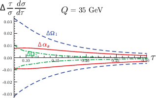
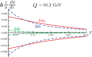
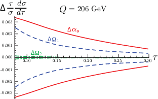
To estimate the theoretical errors in the - plane at any order and for any approximation used for the factorization formula (4), we carry out independent fits for different sets of theory parameters which are randomly chosen in the ranges discussed in the previous sections and summarized in Tab. 3. We take the area covered by the points of the best fits in the - plane as the theory uncertainty treated like -sigma.1313 13 This corresponds to a -sigma error ( CL) in as well as in . We emphasize that this method to estimate theoretical errors is more conservative than the error band method [26] employed for example in Refs. [20, 22]. However, our method required considerably more computer power and it was necessary to use the Tier-2 centers at Garching and MIT, as well as clusters at the MPI and the University of Arizona. In Sec. VII we also present the outcome of other ways to estimate the theoretical error.
It is an important element of our analysis that we carry out global fits to the data from all values of (and all experiments). This is motivated by the strong degeneracy between and in the tail region which can only be lifted when data from different values are simultaneously included in the fits.1414 14 The presence of this degeneracy is presumably also related to why Monte Carlos that are tuned to LEP data tend to have smaller hadronization corrections at than at larger values. See Sec. IX. In Fig. 10 the difference is displayed for and , and GeV. Here is the cross section for the default setting of the theory parameters with and and for we vary either by (solid red curves) or by (dashed blue curves) from their default values. The figures show that in the tail region changes in can be compensated by changes in . This degeneracy makes it impossible to determine and simultaneously with small uncertainties from tail fits that use data from one value (or from a narrow range of values). On the other hand, we see that the correlation is dependent when considering a large enough range of values. In our fits it is particularly important to include, apart from the data from , the low-energy data from JADE, TASSO, and AMY, and the high energy data from the LEP-II experiments. Although the errors in these analyses are larger than from the high-statistics run at LEP-I these data sets are essential for breaking the degeneracy and simultaneously extracting and .
VII Numerical Analysis


Having explained all ingredients of the factorization formula (4) and the fit procedure we are now in the position to discuss the numerical results of our analysis based on a global fit to the experimental data for GeV in the tail region. In the tail region the dominant power corrections are encoded in the first moment , see Eq. (6), so we can determine and from a simultaneous fit. In this section we examine in detail the numerical results of our fits concerning the treatment of the perturbative, hadronization and experimental errors, QED and bottom mass corrections and their dependence on the choice of the data set. We note that the values quoted for in the R-gap scheme are given for reference scales GeV, see Sec. II.6.
| order | (with ) | (with ) |
|---|---|---|
| NLL′ | ||
| NNLL | ||
| NNLL′ | ||
| N3LL | ||
| N3LL′ (full) | ||
| N3LL′ (QCD+) | ||
| N3LL′ (pure QCD) |
| order | () | (R-gap) |
|---|---|---|
| NLL′ | ||
| NNLL | ||
| NNLL′ | ||
| N3LL | ||
| N3LL′ (full) | ||
| N3LL′ (QCD+) | ||
| N3LL′ (pure QCD) |
Theory Scan
In Fig. 11 the best fit points of the theory parameters scan in the - plane are displayed at NLL′ (brown), NNLL (magenta), NNLL′ (green), N3LL (blue) and N3LL′ (red) order. The fit results at N3LL′ order include bottom mass and QED corrections. In Fig. 11a the results in the R-gap scheme with renormalon subtractions are shown, and in Fig. 11b the results in the scheme without gap subtractions are given.
At each order 500 fits were carried out with the theory parameters randomly chosen in the ranges given in Tab. 3. As described in Sec. VI, we take the size of the area in the - plane covered by the best fit points as a measure for the theoretical uncertainties. To visualize the theoretical uncertainties we have colored the respective areas according to the orders. The fit results clearly show a substantial reduction of the theoretical uncertainties with increasing orders. Explicit numerical results for the respective central values (determined by the mean of the respective maximal and minimal values) and the theory errors (determined by half of the difference between maximal and minimal values) for and are given in Tabs. 4 and 5, respectively. We will consider these theory errors as -sigma. At N3LL′ order with in the R-gap scheme the theory error for is compared to with in the scheme. Also at NNLL′ and N3LL we see that the removal of the renormalon leads to a reduction of the theoretical uncertainties by about a factor of two in comparison to the results with in the scheme without renormalon subtraction. The proper treatment of the renormalon subtraction is thus a substantial part of a high-precision analysis for as well as for .

It is instructive to analyze the minimal values for the best fit points shown in Fig. 11. In Fig. 12 the distributions of the best fits in the - plane are shown using the color scheme of Fig. 11. Figure 12a displays the results in R-gap scheme, and Fig. 12b the ones in the scheme. For both schemes we find that the values and the size of the covered area in the - plane systematically decrease with increasing order. While the analysis in the scheme for leads to values around unity and thus an adequate description of the entire global data set at N3LL′ order, we see that accounting for the renormalon subtraction in the R-gap scheme leads to a substantially improved theoretical description having values below unity already at NNLL′ and N3LL orders, with the N3LL′ order result slightly lower at . This demonstrates the excellent description of the experimental data contained in our global data set. It also validates the smaller theoretical uncertainties we obtain for and at N3LL′ order in the R-gap scheme.
As an illustration of the accuracy of the fit, in Fig. 13 we show the theory thrust distributions at for the full N3LL′ order with the R-gap scheme for , for the default theory parameters and the corresponding best fit values shown in bold in Tabs. 4 and 5. The pink band displays the theoretical uncertainty from the scan method. The fit result is shown in comparison with data from DELPHI, ALEPH, OPAL, L3, and SLD, and agrees very well. (Note that the theory values displayed are actually binned according to the ALEPH data set and then joined by a smooth interpolation.)
Band Method
| Band | Band | Our scan | |
|---|---|---|---|
| method 1 | method 2 | method | |
| N3LL′ with | |||
| N3LL′ with | |||
| N3LL′ without | |||
| fixed-order |
It is useful to compare our scan method to determine the perturbative errors with the error band method [26] that was employed in the analyses of Refs. [22, 20, 25]. In the error band method first each theory parameter is varied separately in the respective ranges specified in Tab. 3 while the rest are kept fixed at their default values. The resulting envelope of all these separate variations with the fit parameters and held at their best fit values determines the error bands for the thrust distribution at the different values. Then, the perturbative error is determined by varying keeping all theory parameters to their default values and the value of the moment to its best fit value. The resulting perturbative errors of for our full N3LL′ analysis in the R-gap scheme are given in the first line of Tab. 6. In the second line the corresponding errors for in the scheme for are displayed. The left column gives the error when the band method is applied such that the variation leads to curves strictly inside the error bands for all values. For this method it turns out that the band for the highest value is the most restrictive and sets the size of the error. The resulting error for the N3LL′ analysis in the R-gap scheme is more than a factor of two smaller than the error obtained from our theory scan method, which is shown in the right column. Since the high data has a much lower statistical weight than the data from , we do not consider this method to be sufficiently conservative and conclude that it should not be used. The middle column gives the perturbative error when the band method is applied such that the variation minimizes a function which puts equal weight to all and thrust values. This second band method is more conservative, and for the N3LL′ analyses in the R-gap and the schemes the resulting errors are only smaller than in the scan method that we have adopted. The advantage of the scan method we use is that the fit takes into account theory uncertainties including correlations.
Effects of QED and the bottom mass
Given the high-precision we can achieve at N3LL′ order in the R-gap scheme for , it is a useful exercise to examine also the numerical impact of the corrections arising from the nonzero bottom quark mass and the QED corrections. In Fig. 14 the distributions of the best fit points in the - plane at N3LL′ in the R-gap scheme is displayed for pure massless QCD (light green points), including the bottom mass corrections (medium blue points) and the bottom mass as well as the QED corrections (dark red points). The distribution of the best fit points with bottom mass and QED corrections (dark red points) was already shown in Fig. 11a. The large black dots represent the corresponding central values. The corresponding numerical results are shown at the bottom of Tabs. 4 and 5.

We see that the QED and bottom quark mass effects are somewhat smaller than the theoretical errors of the N3LL′ analysis but not negligible. Moreover we find that the qualitative impact of the QED and the bottom quark mass effects is quite intuitive: The nonzero bottom quark mass primarily causes a horizontal shift of the thrust distribution towards larger values, since the small- threshold for massive quark production is moved to a finite value. Here this is compensated primarily by a reduced value of . Concerning QED effects, they cause an effective increase of the coupling strength in the final state interactions leading primarily to a decrease of in the fit.
As explained in Sec. VI the experimental correction procedures applied to the AMY, JADE, SLC, DELPHI and OPAL data sets were designed to eliminate initial state photon radiation, while those of the TASSO, L3 and ALEPH collaborations eliminated initial and final state radiation. It is straightforward to test for the effect of these differences in the fits by using our theory code with QED effects turned on or off depending on the data set. Since our procedure treats data from different experiments as uncorrelated it is also easy to implement this technically. Using our N3LL′ order code in the R-gap scheme we obtain the central values and GeV, indicated by the hollow circle in Fig. 14. Comparing to our default results given in Tabs. 4 and 5, which are based on the theory code were QED effects are included for all data sets, we see that the central value for is larger by and the one for is smaller by GeV. This shift is substantially smaller than our perturbative error, and justifies our choice to use the theory code with QED effects included as the default code for our analysis.
Hadronization and Experimental Error
An important element in the construction of the function used for our fit procedure is the correlation model for the systematic uncertainties given for the experimental thrust bins. The results discussed above rely on the minimal overlap model for the systematic experimental errors explained in Sec. VI. The -sigma ellipse based on the central values of Eq. (VII) and centered around is shown in Fig. 15 by the red solid ellipse. This ellipse yields the experimental errors and hadronization uncertainty related to in our analysis. We find that the size and correlation coefficients of the -sigma error ellipses at N3LL′ order of all fits made in our theory scan are very similar, and hence we can treat the theory error and these hadronization/experimental errors as independent.
The correlation matrix of the red solid error ellipses is ()
where the correlation coefficient is significant and reads
| (73) |
The numbers in the parentheses represent the variance from the theory scan. From Eq. (VII) it is straightforward to extract the experimental error for and and the error due to variations of and , respectively:
| (74) |
For , the error due to variations is the dominant part of the hadronization uncertainty. The blue dashed ellipse in Fig. 15 shows the total error in our final result quoted in Eq. (76) below.

The correlation exhibited by the red solid error ellipse in Fig. 15 is indicated by the line describing the semimajor axis
| (75) |
Note that extrapolating this correlation to the extreme case where we neglect the nonperturbative corrections () gives . This value is consistent with the fits in Refs. [22, 25] shown in Tab. 1, which are dominated by where the Monte Carlo hadronization uncertainties are smallest.


Individual Theory Scan Errors
It is a useful exercise to have a closer look at the size of the theory uncertainties caused by the variation of each of the theory parameters we vary in our fit procedure in order to assess the dominant sources of theory errors. In Fig. 16 two bar charts are shown for the variation of the best fit values for and at N3LL′ order in the R-gap scheme with our default theory parameters. The bars show individual up-down variations of each of the theory parameters in the ranges given in Tab. 3. The changes of the best fit values related to up variations of the theory parameters are given in dark blue and those related to down variations are given in light green.
We see that the dominant theory uncertainties are related to variations of the profile functions () and the renormalization scale parameter () for the nonsingular partonic distribution . The uncertainties related to the numerical errors of the perturbative constants (, , ) as well as the numerical errors in the extraction of the nonsingular distribution for small values, (, ) are – with the exception of – much smaller and do not play an important role. The theory error related to the unknown 4-loop contribution to the cusp anomalous dimension is negligible. Adding quadratically the symmetrized individual errors shown in Fig. 16 for each parameter, we find for and for . This is about of the theoretical uncertainty we have obtained by the theory parameter scan, and it demonstrates that the theory parameter scan represents a more conservative method to estimate the theory error.
In Fig. 16 we have also shown the variation of the best fit values for and due to variations of the second soft function moment parameter . Our default choice for the parametrization of the soft function uses and with GeV. In this case is the only variable parameter of the soft model function , and is predetermined by Eq. (62) with . As explained in Sec. IV we modify by setting to nonzero values. It is instructive to discuss the values one should consider. From the Cauchy-Schwarz inequality one can show that , giving a strict lower bound on . This bound can only be reached if is a delta-function. Moreover, if is positive definite, vanishing at , has a width of order , has its maximum at a value of order , and has an exponential fall-off for large , then one finds . We therefore adopt the range as a conservative variation to carry out an error estimate. For our default parametrization we have and changing between gives a variation of between and . We find that the best fit values for and are smooth linear functions of which allows for a straightforward extrapolation to the conservative range between and . The results for the variations of the best fit values for and for read and and are also shown in Fig. 16. The symmetrized version of these errors are included in our final results. For our final results for we add the uncertainties from and the one from quadratically giving the total hadronization error. For we quote the error due to separately.
Final Results
As our final result for and , obtained at N3LL′ order in the R-gap scheme for , including bottom quark mass and QED corrections we obtain
| (76) |
where GeV and we quote individual -sigma errors for each parameter. Eq. (76) is the main result of this work. In Fig. 15 (blue dashed line) and Fig. 11a (thick dark red line) we have displayed the corresponding combined total (experimental+theoretical) standard error ellipse. To obtain the combined ellipse we take the theory uncertainties given in Tabs. 4 and 5 together with the uncertainties, adding them in quadrature. The central values in Eq. (76) are determined by the average of the respective maximal and minimal values of the theory scan, and are very close to the central values obtained when running with our default theory parameters. The fit has with a variation of for the displayed scan points. Having added the theory scan and uncertainties reduces the correlation coefficient in Eq. (73) to . As a comparison we have also shown in Fig. 11b the combined total (experimental+theoretical) error ellipse at N3LL′ in the scheme for where the renormalon is not subtracted.
Since our treatment of the correlation of the systematic experimental errors is based on the minimal overlap model, it is instructive to also examine the results treating all the systematic experimental errors as uncorrelated. At N3LL′ order in the R-gap scheme the results that are analogous to Eqs. (76) read and GeV with a combined correlation coefficient of . The results are compatible with the results of Eqs. (76) and indicate that the ignorance of the exact correlation of the systematic experimental errors does not crucially affect the outcome of the fit.
Data Set Choice
We now address the question to which extent the results of Eqs. (76) depend on the thrust ranges contained in the global data set used for the fits. Our default global data set accounts for all experimental thrust bins for in the intervals . (See Sec. VI for more details.) This default global data set is the outcome of a compromise that (i) keeps the interval large to increase statistics, (ii) sets sufficiently large such that the impact of the soft function moments with is small and (iii) takes sufficiently low to exclude the far-tail region where the missing order corrections potentially become important.

In Fig. 17 the best fits and the respective experimental 39% and 68% CL error ellipses for the default values of the theory parameters given in Tab. 3 are shown for global data sets based on different intervals. The results for the various intervals are each given in different colors. The results for our default global data set is given in red color, and the subscript “strict” for some intervals means that bins are included in the data set if more than half their range is contained within the interval. For intervals without a subscript the criterion for selecting bins close to the boundaries of the interval is less strict and generically, if the and values fall in such bins, these bins are included. The numbers in superscript for each of the intervals given in the figure refers to the total number of bins contained in the global data set. We observe that the main effect on the outcome of the fit is related to the choice of and to the total number of bins. Interestingly all error ellipses have very similar correlation and are lined up approximately along the line
| (77) |
Lowering increases the dependence on and leads to smaller and larger values. On the other hand, increasing leads to a smaller data set and to larger experimental error ellipses, hence to larger uncertainties.
It is an interesting but expected outcome of the fits that the pure experimental error for (the uncertainty of for fixed central ) depends fairly weakly on the range and the size of the global data sets shown in Fig. 17. If we had a perfect theory description then we would expect that the centers and the sizes of the error ellipses would be statistically compatible. Here this is not the case, and one should interpret the spread of the ellipses shown in Fig. 17 as being related to the theoretical uncertainty contained in our N3LL′ order predictions. In Fig. 17 we have also displayed the combined (experimental and theoretical) 39% CL standard error ellipse from our default global data set which was already shown in Fig. 11a (and is -sigma, 68% CL, for either one dimensional projection). We also show the 68% CL error ellipse by a dashed red line, which corresponds to -sigma knowledge for both parameters. As we have shown above, the error in both the dashed and solid larger ellipses is dominated by the theory scan uncertainties, see Eqs. (76). The spread of the error ellipses from the different global data sets is compatible with the -sigma interpretation of our theoretical error estimate, and hence is already represented in our final results.
Analysis without Power Corrections
| (pert. error) | ||
|---|---|---|
| N3LL′ with | ||
| N3LL′ with | ||
| N3LL′ without | ||
| fixed-order without |
Using the simple assumption that the thrust distribution in the tail region is proportional to and that the main effect of power corrections is a shift of the distribution in , we have estimated in Sec. I that a power correction will lead to an extraction of from data that is lower than an analysis without power corrections. In our theory code we can easily eliminate all nonperturbative effects by setting and . At N3LL′ order and using our scan method to determine the perturbative uncertainty a global fit to our default data set yields which is indeed larger than our main result in Eq. (76) which accounts for nonperturbative effects. It is also interesting to do the same fit with a purely fixed-order code, which we can do by setting to eliminate the summation of logarithms. The corresponding fit yields , where the displayed error has again been determined from the theory scan which in this case accounts for variations of and the numerical uncertainties associated with and . (A comparison with Ref. [22] is given below in Sec. IX.)
These results have been collected in Tab. 7 together with the results of our analyses with power corrections in the R-gap and the schemes. For completeness we have also displayed the respective values which were determined by the average of the maximal and the minimum values obtained in the scan.
VIII Far-tail and Peak Predictions


The factorization formula (4) can be simultaneously used in the peak, tail, and far-tail regions. To conclude the discussion of the numerical results of our global analysis in the tail region, we use the results obtained from this tail fit to make predictions in the peak and the far-tail regions.
In Fig. 18 we compare predictions from our full N3LL′ code in the R-gap scheme (solid red line) to the accurate ALEPH data at in the far-tail region. As input for and we use our main result of Eq. (76) and all other theory parameters are set to their default values (see Tab. 3). We find excellent agreement within the theoretical uncertainties (pink band). Key features of our theoretical result in Eq. (4) that are important in this far-tail region are i) the nonperturbative correction from , and ii) the merging of , , and toward at in the profile functions, which properly treats the cancellations occurring at multijet thresholds. To illustrate the importance of we show the long-dashed red line in Fig. 18 which has the same value of , but turns off the nonperturbative corrections. To illustrate the importance of the treatment of multijet thresholds in our profile function, we take the BS profile which does not account for the thresholds (the BS profile is defined and discussed below in Sec. IX), and use the smaller and larger that are obtained from the global fit in this case. The result is shown by the solid light blue line in Fig. 18, which begins to deviate from the data for and gives a cross section that does not fall to zero at . The fact that is smaller by for the light blue line, relative to the solid red line, indicates that the proper theoretical description of the cross section in the far-tail region has an important impact on the fit done in the tail region. The final curve shown in Fig. 18 is the short-dashed green line, which is the result at the level of precision of the analysis by Becher and Schwartz in Ref. [20]. It uses the BS profile, has no power corrections, and has the value of obtained from the fit in Ref. [20]. It also misses the data in this region. The results of other thrust analyses, such as Davison and Webber [23] and Dissertori et al. [22, 25], significantly undershoot the data in this far-tail region.1515 15 See the top panel of Fig. 9 in Ref. [23], the top left panel of Fig. 4 in Ref. [22], and the left panel of Fig. 2 in Ref. [25]. To the best of our knowledge, the theoretical cross section presented here is the first to obtain predictions in this far-tail region that agree with the data. Note that our analysis does include some power corrections through the use of Eq. (24). It does not account for the full set of power corrections as indicated in Eq. (4) (see also Tab. 2b), but the agreement with the experimental data seems to indicate that missing power corrections may be smaller than expected.
Unbinned predictions for the thrust cross section at in the peak region are shown in Fig. 19. The green dashed curve shows the result at the level of precision in Becher and Schwartz, that is N3LL′, with the BS profile, without power corrections, and with the value of obtained from their fit. This purely perturbative result peaks to the left of the data. With the smaller value of obtained from our fit, the result with no power corrections peaks even slightly further to the left, as shown by the long-dashed red curve. In contrast, the red solid curve shows the prediction from our full N3LL′ code in the R-gap scheme with our central fit values of and given in Eq. (76). It clearly indicates that the value of obtained from the fit in the tail region shifts the theory prediction in the peak region much closer to the experimental data. The residual difference between the solid red theory curve and the experimental data can be attributed to the fact that the peak is sensitive to power corrections from higher moments, , which have not been fit in our analysis. In our theoretical cross section result this would correspond to fitting , and a subset of the higher coefficients . The were all set to zero in the curves shown here, and we leave the presentation of results of this extended fit to a future publication.
IX Cross checks and Comparisons
The result for we obtain from our global N3LL′ analysis in the R-gap scheme with 487 bins given in Eq. (76) is consistent at -sigma with the result of Davison and Webber [23] (). They also carried out a global thrust analysis with a total of 430 experimental bins. As explained in Sec. I, in their theory formula nonperturbative effects were included as a power correction in the effective coupling model which was fit from the experimental data, and their approach also accounts for a renormalon subtraction of the perturbative distribution. In these respects their analysis is similar to ours. However, it differs as their theory formula contains only resummation of logarithms at NLL order, and it also uses a different renormalon subtraction scheme which is based on the running coupling approximation for the subtraction corrections and does not account for the resummation of large logarithms. Moreover the separation of singular and nonsingular perturbative contributions and method to turn off the log resummation at large is not equivalent to the one we employ. The difference between their central value and perturbative error and our Eq. (76) can be attributed to these items. Their combined hadronization and experimental uncertainty utilizes an error rescaling using the value obtained for their best fit.
On the other hand, our main result for given in Eq. (76) is smaller than the results of Dissertori et al. [22] by -sigma, of Dissertori et al. [25] by -sigma, and of Becher and Schwartz [20] by -sigma. (These results are displayed in Table 1.) In these analyses was determined from fits to data for individual values and, as explained in Sec. I, nonperturbative corrections and their associated uncertainty were taken from Monte Carlo generators in Dissertori et al., or left out from the fit and used to assign the hadronization uncertainty for the final result in Becher and Schwartz. It is possible to turn off pieces of our theoretical code to reproduce the perturbative precision of the codes used in Refs. [22]1616 16 We do not attempt to reproduce the NLL/ code of Ref. [25] as the final outcome is similar to Ref. [22]. and [20]. It is the main purpose of the remainder of this section to show the outcome of the fits based on these modified theory codes. We show in particular, that the main reason why the above results for are higher than our result of Eq. (76) is related to the fact that the nonperturbative corrections extracted from Monte Carlo generators at are substantially smaller than and incompatible with the ones obtained from our fit of the field theory power correction parameter . In Sec. I we already discussed why the use of Monte Carlo generators to estimate nonperturbative corrections in high-precision perturbative predictions is problematic.
| BS | our BS | default | ||
| Experiment | Energy | results [20] | profile | profile |
| ALEPH | GeV | |||
| ALEPH | GeV | |||
| ALEPH | GeV | |||
| ALEPH | GeV | |||
| ALEPH | GeV | |||
| ALEPH | GeV | |||
| ALEPH | GeV | |||
| ALEPH | GeV | |||
| OPAL | GeV | |||
| OPAL | GeV | |||
| OPAL | GeV | |||
| OPAL | GeV | |||
| average | ||||
| global fit (stat) | all | |||
| global fit (stat+syst) | all |
We start with an examination related to the code used by Becher and Schwartz [20], which has N3LL′ accuracy but does not include power corrections or renormalon subtractions. This treatment can be reproduced in our factorization formula by turning off the nonperturbative soft nonperturbative function by setting and . Moreover they used the central scale setting , and . We can reproduce this from our profile functions for , and , which we call the BS profile setting. The BS profile functions for and are shown by dashed curves in Fig. 8. (Note that the BS profile setting does not cause , , and to merge in the far-tail region and become equal at , which is needed to switch off the SCET resummation of logarithms in the multijet region to satisfy the constraints from multijet thresholds.) Becher and Schwartz set the nonlogarithmic correction in the Euclidean hard factor to zero (with for ), which in our notation corresponds to (somewhat larger than the now known ). We also set (see Ref. [62, 20]) and for the non-logarithmic and constants in the soft function (both within our range of uncertainties). The value for corresponds to setting the nonlogarithmic corrections in the expanded position space soft function to zero. Finally, we also turn off our QED and bottom quark mass corrections and the axial singlet corrections, and use the fixed-order normalization from Eq. (64). For the fit procedure we follow Becher and Schwartz and analyze all ALEPH and OPAL data for individual values in the ranges given in their work and account only for statistical experimental errors in the functions. The outcome of the fits for at N3LL′ order is given in the fourth column of Tab. 8. The third column shows their central values and the respective statistical experimental errors as given in Ref. [20]. The numbers we obtain are to higher than their central values, and we attribute this discrepancy to the nonsingular contributions.1717 17 Becher and Schwartz uncovered a numerical problem with the original EERAD3 code at very small , which correspondingly had an impact on the nonsingular function used in their analysis which was extracted from EERAD3. When their nonsingular distribution is updated to results from the new EERAD3 code they become significantly closer to ours, differing by . We thank M. Schwartz for correspondence about this and for providing us with their new fit values. (Becher and Schwartz also used a difference of cumulants for their fits, as in Eq. (67) with the choice and , rather than integrating as we do for the table. The spurious contribution induced by this choice has a significant effect on the values, but a small effect on , changing the values shown in the table by . For cumulants that use with no spurious contribution, the difference from our integrated distribution results is reduced to for , and values are almost unaffected.)
The numbers obtained at N3LL′ above are significantly larger than our central fit result shown in Eq. (76) obtained from our full code. These differences are mainly related to the nonperturbative power correction and partly due to the BS profile setting. To distinguish these two and other effects we can take the purely perturbative code described above and turn back to our default setting for the profile functions with the parameters given in Tab. 3. The results are shown in the fifth column in Tab. 8 using again only statistical experimental errors in the functions. The values using our default profile functions are by to larger than for the BS profile setting in the fourth column.1818 18 With our full code, which accounts in particular for power corrections and renormalon subtractions, the shift due to the modified profile functions becomes smaller; shifts in of become . (The fifth column results again integrate the distribution over each bin rather than using differences of cumulants, which for our profile is important for the reasons discussed in Sec. V.1919 19 Using the cumulant method with and in Eq. (67), which has a spurious contribution, changes the values in the fifth column of Tab. 3 by about to . On the other hand, using the cumulant method without a spurious contribution, , changes the values in the fifth column by . ) A similar difference arises from a global fit to our default data set of Sec. VI using the same fit procedure: For the BS profile setting we obtain , while the default profile setting gives (second to last line of Tab. 8). Using instead the -analysis of our main analysis which includes the experimental systematical errors we obtain for the BS profile setting and for the default profile setting (last line of Tab. 8). The latter result is by larger than our central fit result in Eq. (76). This 10% effect is almost entirely coming from the power correction . The difference of to the full perturbative result of given in Table 7 illustrates the combined effect of the QED, the bottom quark mass and the axial singlet corrections and the hard constant .
Finally, let us examine the results related to the code used by Dissertori et al. in Ref. [22], which uses the fixed-order results without a resummation of logarithms, but accounts for nonperturbative corrections determined from the difference of running Monte Carlo generators in parton and hadron level modes. Since in this work we are not concerned with extracting the parton-hadron level transfer matrix from Monte Carlo generators, we use in the following our code neglecting power corrections by setting , setting , and setting . The latter switches off the log resummation factors in Eq. (4) such that only the fixed order expression remains. We also include the corrections, but neglect QED effects. Since these modifications give us a code that does not contain nonperturbative corrections, the differences to Ref. [22] we obtain will serve as a quantitative illustration for the size of the hadronization corrections obtained by a transfer matrix from the Monte Carlo generators PYTHIA, HERWIG, and ARIADNE, tuned to global hadronic observables at .
| Dissertori et al. | Our fixed | ||
|---|---|---|---|
| Experiment | Energy | results [22] | order code |
| ALEPH | GeV | ||
| ALEPH | GeV | ||
| ALEPH | GeV | ||
| ALEPH | GeV | ||
| ALEPH | GeV | ||
| ALEPH | GeV | ||
| ALEPH | GeV | ||
| ALEPH | GeV |
For the fits for we follow Dissertori et al. [22] analyzing ALEPH data for individual values in the ranges given in their work and accounting only for statistical experimental errors in the functions. The results of Dissertori et al. and the outcome for our best fits are given in the third and fourth column of Tab. 9, respectively. We have also quoted the respective statistical errors from Ref. [22]. For the high statistics data at our result is larger than theirs, but the discrepancy amounts to only which is a shift in . This illustrates the small size of the nonperturbative hadronization corrections encoded in the Monte Carlo transfer matrix at . This is clearly incompatible with the size of the nonperturbative correction we have obtained from simultaneous fits of and , confirming the concerns on Monte Carlo hadronization corrections explained in Sec. I. Interestingly, with the exception of , our fixed-order results for all are relatively stable and close to the result at , while their values, which use the transfer matrix for nonperturbative effects, are systematically lower for by to . Thus the nonperturbative effects from the Monte Carlo transfer matrix are substantially larger for .2020 20 Note that the weighted average of the thrust results of Dissertori et al. is and is consistent with our result in Eq. (76) within the larger uncertainties. Also note that the dependence of our power correction is affected by its anomalous dimension, cf. Fig. 6. The same behavior is also visible in the results of Ref. [25], which includes NLL resummation of logarithms. Since the transfer matrix is obtained from Monte Carlo tuned to the more accurate data, we believe that this issue deserves further investigation. To complete the discussion we use the same fixed-order theory code to quote results for a global fit to our default data set. Using the fit procedure as described in Sec. VI we obtain . (The corresponding errors obtained from the error band method are given in the fourth line of Tab. 6.)

X Conclusions
In this work we have provided a factorization formula for the thrust distribution in annihilation which incorporates the previously known and perturbative QCD corrections and summation of large logarithms at N3LL order for the singular terms in the dijet limit where the thrust variable is small. The factorization formula used here incorporates a systematic description of nonperturbative effects with a soft function defined in field theory. The soft function describes the dynamics of soft particle radiation at large angles. We have also accounted for bottom mass and QED photon effects for fixed-order contributions as well as for the summation of QED logarithms. With specifically designed -dependent profile functions for the renormalization scales the factorization formula can be applied in the peak, tail and far-tail regions of the thrust distribution. It has all nonperturbative effects accounted for up to terms of , which is parametrically smaller than the remaining perturbative uncertainty ( for ) of the thrust distribution predictions in the tail region where we carried out the fits to the experimental data.
In the tail region, , the dominant effects of the nonperturbative soft function are encoded in its first moment , which is a power correction to the cross section. Fitting to tail data at multiple s as we did in this work, the strong coupling and the moment can be simultaneously determined. An essential ingredient to reduce the theoretical uncertainties to the level of in the thrust distribution is our use of a short-distance scheme for , called the R-gap scheme, that induces subtractions related to an renormalon contained in the perturbative thrust cross section from large angle soft gluon radiation. The R-gap scheme introduces an additional scale that leads to large logarithms in the subtractions, and we carry out a summation of these additional logarithms with renormalization group equations in the variable . The R-gap scheme reduces the perturbative uncertainties in our best highest order theory code by roughly a factor of two compared to the pure definition, , where renormalon effects are not treated.
The code we use in this analysis represents the most complete theoretical treatment of thrust existing at this time. As our final result we obtain
| (78) |
where is defined in the scheme, and in the R-gap scheme at the reference scales GeV. Here the respective total -sigma errors are shown. The results with individual -sigma errors quoted separately for the different sources of uncertainties are given in Eq. (76). Neglecting the nonperturbative effects incorporated in the soft function, and in particular , from the fits gives which exceeds the result in Eq. (78) by . This is consistent with a simple scaling argument one can derive from experimental data, see Eq. (3) in Sec. I.
Analyses of event shapes with a simultaneous fit of and a power correction have been carried out earlier with the effective coupling model. Davison and Webber [23] analyzed the thrust distribution and determined also using fixed-order input, but implementing the summation of logarithms only at NLL order (for further discussion see Sec. IX). Recently Gehrmann et al. [95] analyzed moments of different event shape distributions, also with the effective coupling model, and obtained using fixed-order perturbation theory at . Both analyses neglected bottom mass and QED corrections. Our result in Eq. (78) is compatible with these analyses at -sigma, but has smaller uncertainties.
These results and our result for in Eq. (78) are substantially smaller than the results of event shape analyses employing input from Monte Carlo generators to determine nonperturbative effects. We emphasize that using parton-to-hadron level transfer matrices obtained from Monte Carlo generators to incorporate nonperturbative effects is not compatible with a high-order theoretical analysis such as ours, and thus analyses relying on such Monte Carlo input contain systematic errors in the determination of from thrust data. The small effect of hadronization corrections on thrust observed in Monte Carlo generators at and the corresponding small shift in do not agree with the shift we have obtained from our fits as mentioned above. For the reasons discussed earlier, we believe Monte Carlo should not be used for hadronization uncertainties in higher order analyses.
Although our theoretical approach represents the most complete treatment of thrust at this time, and all sources of uncertainties known to us have been incorporated in our error budget, there are a number of theoretical issues related to subleading contributions that deserve further investigation. These issues include (i) the summation of logarithms for the nonsingular partonic cross section, (ii) the structure of the power corrections, (iii) analytic perturbative computations of the and nonlogarithmic coefficients and in the partonic soft function, the nonlogarithmic coefficient in the partonic jet function, and the 4-loop QCD cusp anomalous dimension . Concerning issue (i) we have incorporated in our analysis the nonsingular contributions in fixed-order perturbation theory and estimated the uncertainty related to the higher order logarithms through the usual renormalization scale variation. Further theoretical work is needed to derive the renormalization group structure of subleading jet, soft, and hard functions in the nonsingular contributions and to use these results to sum the corresponding logarithms. Concerning issue (ii) we have shown that our theoretical description for the thrust distribution contains a remaining theoretical uncertainty from nonperturbative effects of order . Parametrically, this uncertainty is substantially smaller than the perturbative error of about for the thrust distribution in the tail region at LEP-I energies that is contained in our best theory code. Furthermore, our predictions in the far-tail region at appear to indicate that the dominant corrections of this order are already captured in our setup. Nevertheless a systematic analysis of these subleading effects is certainly warranted.
Apart from investigating these theoretical issues, it is also warranted to apply the high-precision approach using soft-collinear effective theory to other event shape distributions in order to validate the result in Eq. (78). Event shapes that can be clearly treated with similar techniques are: heavy and light jet masses, the C-parameter, and the angularities [96, 97]. For many of these event shapes it has been proven field theoretically that the same parameter describes the leading power corrections in the tail region [65], although there might be caveats related to the experimental treatment of hadron masses [98, 37]. Thus, one has the potential to extend the analysis done here to include additional data without additional parameters. An analysis for the heavy jet mass accounting for perturbative contributions at N3LL in with different profile functions and a simple soft function model for power corrections without renormalon subtractions, was recently carried out in Ref. [99], providing a first step in this direction.
To conclude this work we cannot resist comparing our result for with the results of a selection of analyses using other techniques and observables, as shown in Fig. 20. We include a N3LO analysis of data from deep inelastic scattering in the nonsinglet channel [100]2121 21 Analyses studying with data that depends also on the gluon PDF have been carried out in Refs. [101, 102, 103, 104]., the recent HPQCD lattice determination based on fitting Wilson loops and the - mass difference [105], the result from fits to electroweak precision observables based on the Gfitter package [106], analyses of -decay data using fixed-order [107] and contour-improved perturbation theory [108], together with an average of results from Ref. [109]. Finally we also show a collection of -averages from Refs. [109, 110, 111]. The DIS result is consistent with our fit result, whereas the deviation from HPQCD is . It is interesting to note that the high energy extractions from thrust and DIS appear to be smaller than the low energy extractions from Lattice and decays.
Acknowledgements.
This work was supported in part by the Director, Office of Science, Office of Nuclear Physics of the U.S. Department of Energy under the Contracts DE-FG02-94ER40818, DE-FG02-06ER41449, and the European Community’s Marie-Curie Research Networks under contract MRTN-CT-2006-035482 (FLAVIAnet) and MRTN-CT-2006-035505 (HEPTOOLS). IS was also supported in part by the DOE OJI program, the Sloan Foundation, and by a Friedrich Wilhelm Bessel award from the Alexander von Humboldt foundation. VM has been partially supported by a DFG “Eigenen Stelle” under contract MA 4882/1-1. MF was supported in part by the German Academic Exchange Service (DAAD) D/07/44491. RA, MF and IS thank the Max-Planck Institute for Physics for hospitality while parts of this work were completed. We thank Thomas Gehrmann for useful conversations on the experimental treatment of photon radiation and in particular for providing us with the most up-to-date numerical results from the program EERAD3 that made our N3LL′ analysis possible. We are particularly indebted to Stefan Kluth for countless valuable discussions and information on experimental data and the usage of the program EVENT2. We are grateful to Daniel Wicke for useful discussions concerning the treatment of experimental data. We thank Thomas Hahn for computing support. MF thanks Sean Fleming for scientific advice. We thank T. Gehrmann, S. Kluth, M. Schwartz, and F. Tackmann for comments on the manuscript. We thank the Aspen Center for Physics for a stimulating environment when this work was finalized.Appendix A Formulae
In this appendix we collect all the remaining formulas used in our analysis for the case of massless quarks. The total hadronic cross section at tree level at the energies we are considering is
| (79) |
where Q is the c.m. energy. For a quark of flavor the tree level axial-vector and vector cross sections are
| (80) | |||||
where is the electric charge of the quark, and
| (81) |
Here is the third component of the weak isospin, and is the weak mixing angle. For our numerics we use the following values:
| (82) |
Singular Cross Section Formula
To simplify the numerical evaluation of the singular part of the differential cross section given in Eq. (11) we take so that and express the result in the following form
| (83) |
where the perturbative corrections from the partonic soft function, jet function, and soft evolution factor are contained in . The integrals in can be carried out explicitly so that it is given by a simple set of functions. The soft nonperturbative function is discussed in Sec. IV, and in Eq. (83) we have integrated by parts so the derivative in the exponential with the acts on this nonperturbative function. , , and (cf. Eq. (37)) involve series in , , and with no large logs, and in our numerical analysis we expand the product of these series out, order-by-order in . This expansion is crucial for and since it is needed to allow the renormalon in the two series to cancel.
For simplicity where possible we give ingredients in a numerical form for SU(3) color with active flavors. The vector hard function to is [48, 49, 50, 51, 52, 42]
| (84) |
where and from Eq. (12) we have . Our axial-vector hard function for quarks has an extra two-loop singlet piece from the large top-bottom mass splitting, . was given in Eq. (13) and involves the real function [56]
| (85) |
where and
| (86) |
The resummation of large logs from to is given by in Eq. (83) which is the solution of the RGE for the square of the SCET Wilson coefficient [8]
| (87) |
and the functions and are given in Eqs. (101) and (102) below.
Finally using results for the convolution of plus-functions from Ref. [38] we have the momentum space formula
| (88) |
This result is independent of the dummy variable .2222 22 When convoluted with we evaluate the right-hand side of Eq. (88) for which simplifies the final numerical integration. Here encodes part of the running between the jet and the soft scale [112, 113],
| (89) | ||||
The sum in Eq. (88) contains coefficients of the momentum space soft and jet functions. Shifting the plus-functions so that they have common arguments gives
| (90) |
Here the thrust soft function coefficients are
| (91) |
The soft function is known to except for the constant term [15, 14, 20, 62]
| (92) |
Note that and are the coefficients of the non-logarithmic terms in the series expansion of the logarithm of the position space thrust soft function. The coefficients appearing in the shifted thrust jet function are
| (93) |
and are known up to except for the constant term [58, 59, 114, 60, 61, 20]
| (94) |
The distributions are defined as []
| (95) |
, and for
| (96) |
In Eq. (88) we use the coefficients [38]
| (97) |
and the coefficients
| (98) |
where
| (99) |
Special cases not covered by the general formulae in Eqs. (97) and (98) include
| (100) |
Evolution factors and Anomalous Dimensions
The evolution factors appearing in Eqs. (87), (88), and (89) are
| (101) |
and
| (102) |
where depends on 4-loop running couplings, and the coefficients are and . These results are expressed in terms of series expansion coefficients of the QCD function , of which is given by a constant of proportionality times the QCD cusp anomalous dimension, and of a non-cusp anomalous dimension ,
| (103) | ||||
The coefficients for are [115, 116, 117, 118, 61, Czakon:2004bu]
| (104) | ||||
For the unknown four-loop cusp anomalous dimension we use the Padè approximation assigning 200% uncertainty:
| (105) |
The anomalous dimensions for the hard, jet, and soft functions are [21, 119, 61, 113, 51, 120, 121]
| (106) |
To determine the strong coupling in terms of at -loops with 5 light flavors we use
| (107) | ||||
where and the displayed numbers are determined from the in Eq. (104). The form in Eq. (107) agrees very well with the numerical solution of the beta function equation.
Nonsingular Cross Section Formula
At there is an axial singlet contribution to the nonsingular terms through the three-parton cut of Fig. 2, which is given by the function appearing in Eq. (27) for . The result for this function can be extracted from results in Ref. [70] and reads: []
| (108) | ||||
R-evolution
Finally we display here the function [39] which appears in the solution in Eq. (41) of the R-RGE equation for :
| (109) |
which is real since the complex phase cancels the imaginary part coming from the incomplete Gamma functions, defined as
| (110) |
Here is the order of the matrix elements (that is for NLL′ and NNLL, for NNLL′ and N3LL, and for N3LL′. For lower orders ). In Eq. (109) we have defined
| (111) |
where the R-anomalous dimensions were given in Eq. (40).
Total Hadronic Cross Section
The total hadronic QCD cross section, can be evaluated in fixed-order perturbation theory with , and was given in Eq. (63) with the vector QCD results given in Eq. (64). The function appearing in the singlet contribution in Eq. (63) at is [56]
| (112) |
where the necessary functions appear in Eq. (86). Note that we have dropped the four particle cut contribution since we have not accounted for it in the nonsingular distribution.
Appendix B Soft Function OPE Matching
To derive Eq. (21) we must demonstrate uniqueness of the power correction and derive its perturbative Wilson coefficient to all orders in . We carry out these two parts of the proof in turn.
Since the operator appearing in the matrix element is non-local, the proof of uniqueness is more involved than for a typical OPE where we could just enumerate all local operators of the appropriate dimension. Here we are integrating out perturbative soft gluons in , while retaining nonperturbative soft gluons. The hierarchy between these soft gluons is in their invariant masses, . This process can not introduce Wilson lines in new light-like directions, nor additional Wilson lines following paths in and . Thus the Wilson lines will be the same as those in the full theory operator, Eq. (17). Additional Wilson lines could only be induced by integrating out collinear or hard gluons, which would yield power corrections suppressed by the hard or jet scales. The second point to demonstrate is that dimension one combinations of derivatives other than do not lead to new nonperturbative matrix elements at this order. The key is that for derivative operators inside our vacuum matrix element involving Wilson lines, boost invariance along the thrust axis relates all matrix elements to [65]. The proof relies on boost invariance along the thrust axis of derivative operators inside the vacuum matrix element. To see this one defines the transverse energy flow operator by its action on states [18, 47]
| (113) |
Any dimension one derivative operator we might wish to consider, such as , , , , , or combinations thereof, are given by an integral for an appropriate rapidity function . For example, for the thrust derivative we have . Boost invariance implies [65]
| (114) |
for arbitrary . The same steps hold for any other derivative operator and function , and different choices only affects the constant calculable prefactor. This suffices to show the second point.
To derive an all orders expression for the Wilson coefficient of we construct an analog of the OPE matching done for the soft function in [59]. The proof is considerably simpler for because the OPE in that case yields local HQET operators. Nevertheless the thrust soft function can be manipulated such that a similar strategy can be used. Using the thrust axis we define hemisphere where and hemisphere where . Consider the soft function written as a matrix element squared
| (115) |
where the trace is over color, is the total plus-momentum of the particles in state in hemisphere and is the minus-momenta of particles in in hemisphere . To carry out the OPE we need to consider a state that has overlap with the operator in Eq. (20). Thus we could replace the vacuum by very soft nonperturbative gluons with momenta of and then consider matrix elements with perturbative gluons having momenta . Since the OPE is independent of the particular states we choose, we will instead consider a simpler alternative in the following.
First we write the matrix element in Eq. (115) as
| (116) | ||||
where and are non-interacting collinear fields whose contractions with the sterile quark and anti-quark are chosen with a normalization to reproduce the original matrix element (and a sum over their color correctly reproduces the trace). Here should be thought of as a very energetic collinear quark in hemisphere with large label momentum , and zero residual momentum. The large momentum is conserved by soft interactions from the Wilson lines due to the SCET multipole expansion. Here the plus-momentum of is included into , but is zero and does not contribute to the -function. The same is true for which has zero minus-momentum, large label momentum, and is always in hemisphere . We introduced and so that we can use them to systematically add a very soft momentum to the end of the Wilson lines (at ). They provide a convenient state with which to carry out the OPE, because there is nonzero overlap taking only the out of the Wilson lines, . In particular they allow us to perform the OPE and pick out the present in at tree level, without the necessity to add explicit soft gluons with momenta .
To carry out the OPE we now give a very small soft momentum and a very small soft momentum , and denote them by and respectively. These particles are kept on-shell by adjusting their large label -momenta so that and . Due to the multipole expansion these -momenta have no influence on diagrams with perturbative soft gluons having momenta . The Wilson line propagators reduce to the same as before, such as
| (117) |
This property is familiar in SCET where soft couplings to energetic collinear quarks in SCET remain eikonal for any values of the quark’s large momenta by using the equations of motion, as long as the final particles are on-shell. Thus at any order in perturbation theory, with any number of soft gluons and soft quarks of momenta in the matrix elements, the only change caused by is on the in Eq. (115) which is shifted to , where . Expanding with the matrix element with this choice of state evaluates to
| (118) |
At lowest order in emission of very soft gluons the corresponding matrix element in the lower energy theory is
| (119) |
Virtual radiative corrections do not correct this result since they are scaleless and vanish in pure dimensional regularization. Thus we can identify in Eq. (118), and this then yields the stated result for the OPE in Eq. (21).
Appendix C Operator Expansion for the First Thrust Moment

For moment integrals of the thrust distribution over there is not a hierarchy of scales that induces large logs, and one may formulate the theoretical result in terms of an expansion in and . The zero’th moment of thrust is just the total cross section for , and the power corrections are formulated in terms of the well known OPE [122]. For higher moments the fact that thrust constrains a non-trivial combination of final state momenta makes carrying out an OPE more difficult. For example, when we weigh the integral by a power of thrust it is not possible to collapse all propagators to a point, so the nonperturbative parameters are no longer constrained to be given by a basis of local operators. In the effective coupling model [35] the same nonperturbative parameter that appears for the thrust distribution, also occurs in the first moment. However it is not clear to what level of accuracy this carries over to a field theoretical description of power corrections derived from QCD. In this appendix we show how one can carry out an OPE for the 1st moment of the thrust distribution, and demonstrate that at leading order it only involves the same nonperturbative matrix element from Eq. (6).
To carry out an OPE for the thrust moment we can work order by order in the hard expansion, and analyze direct computations where we couple soft nonperturbative gluons to hard partons in Feynman diagrams. The appropriate non-local operator(s) appearing in the expansion will be identified by the structure of the amplitudes in this computation. In the following discussion the soft gluons will not be treated as final state particles for which there is a phase space integral, but rather as a means of probing the structure of the nonperturbative operator. The lowest order graphs with zero or one soft gluon and a virtual photon current (for simplicity) are shown in Fig. 21. Here is soft, and , are hard momenta. To carry out the OPE we calculate and square the on-shell amplitude, , where , are the virtual photon current indices. We sum over the final quark/antiquark spins since these particles are hard and are being integrated out. On the other hand the gluon vector indices , are left uncontracted and are used to help in identifying the operator for the nonperturbative matrix element. For simplicity, the indices and are suppressed in writing down the amplitudes below. We start out without making restrictions on the number of gluons coming from and , which corresponds to directly matching onto the nonperturbative operator, without considering the final vacuum matrix element which gives a nonperturbative parameter. Since the denominators of the propagators in the one gluon graphs reduce to and . In the numerators we can drop ’s relative to the large and . The interference between the zero and one gluon amplitudes gives
| (120) |
The interference with one gluon from each of and is
| (121) | ||||
Continuing in this fashion with any number of gluons from and any number from we always find the tree level amplitude squared with no soft gluons, , times an amplitude from the soft gluons.
Since the hard quarks are on-shell and back-to-back their four-momenta are given by light-like vectors along the thrust axis,
| (122) |
up to power corrections beyond those considered here. Here and are identical to the and appearing in Eq. (6). Using Eq. (122) the soft gluon amplitudes in Eqs. (120) and (121) are eikonal with precisely the right factors to come from the , , , in the matrix element in Eq. (6).
For the first moment observable we can focus on amplitudes that have the same number of gluons in and , and at least one gluon for the operation in Eq. (6) to act on. Since the gluon is soft, the factor of in is given by
| (123) | ||||
and is exactly equal to given in Eq. (7) acting on the soft gluon in Fig. 21. Hence in the first moment of thrust we find that together with the soft gluon amplitude give precisely , with the vacuum matrix in Eq. (6) (where the trace comes from the sum over color for the final state quarks). The remaining amplitude goes together with the two-body phase space to yield the tree level cross section . Together these results yield Eq. (25) for the lowest order OPE for the first moment of thrust.
References
- [1] S. Kluth, Rept. Prog. Phys. 69, 1771 (2006), eprint hep-ex/0603011.
- [2] E. Farhi, Phys. Rev. Lett. 39, 1587 (1977).
- [3] A. Gehrmann-De Ridder, T. Gehrmann, E. W. N. Glover, and G. Heinrich, Phys. Rev. Lett. 99, 132002 (2007a), eprint 0707.1285.
- [4] A. Gehrmann-De Ridder, T. Gehrmann, E. W. N. Glover, and G. Heinrich, JHEP 12, 094 (2007b), eprint 0711.4711.
- [5] S. Weinzierl, Phys. Rev. Lett. 101, 162001 (2008), eprint 0807.3241.
- [6] S. Weinzierl, JHEP 06, 041 (2009), eprint 0904.1077.
- [7] C. W. Bauer, S. Fleming, and M. E. Luke, Phys. Rev. D 63, 014006 (2001a), eprint hep-ph/0005275.
- [8] C. W. Bauer, S. Fleming, D. Pirjol, and I. W. Stewart, Phys. Rev. D 63, 114020 (2001b), eprint hep-ph/0011336.
- [9] C. W. Bauer and I. W. Stewart, Phys. Lett. B 516, 134 (2001), eprint hep-ph/0107001.
- [10] C. W. Bauer, D. Pirjol, and I. W. Stewart, Phys. Rev. D65, 054022 (2002a), eprint hep-ph/0109045.
- [11] C. W. Bauer, S. Fleming, D. Pirjol, I. Z. Rothstein, and I. W. Stewart, Phys. Rev. D 66, 014017 (2002b), eprint hep-ph/0202088.
- [12] C. W. Bauer, A. V. Manohar, and M. B. Wise, Phys. Rev. Lett. 91, 122001 (2003), eprint hep-ph/0212255.
- [13] C. W. Bauer, C. Lee, A. V. Manohar, and M. B. Wise, Phys. Rev. D 70, 034014 (2004), eprint hep-ph/0309278.
- [14] S. Fleming, A. H. Hoang, S. Mantry, and I. W. Stewart, Phys. Rev. D77, 074010 (2008a), eprint hep-ph/0703207.
- [15] M. D. Schwartz, Phys. Rev. D77, 014026 (2008), eprint 0709.2709.
- [16] A. H. Hoang and I. W. Stewart, Phys. Lett. B660, 483 (2008), eprint 0709.3519.
- [17] G. P. Korchemsky (1998), eprint hep-ph/9806537.
- [18] G. P. Korchemsky and G. Sterman, Nucl. Phys. B555, 335 (1999), eprint hep-ph/9902341.
- [19] G. P. Korchemsky and S. Tafat, JHEP 10, 010 (2000), eprint hep-ph/0007005.
- [20] T. Becher and M. D. Schwartz, JHEP 07, 034 (2008), eprint 0803.0342.
- [21] S. Catani, L. Trentadue, G. Turnock, and B. R. Webber, Nucl. Phys. B407, 3 (1993).
- [22] G. Dissertori et al., JHEP 02, 040 (2008), eprint 0712.0327.
- [23] R. A. Davison and B. R. Webber, Eur. Phys. J. C59, 13 (2009), eprint 0809.3326.
- [24] S. Bethke, S. Kluth, C. Pahl, and J. Schieck (JADE), Eur. Phys. J. C64, 351 (2009), eprint 0810.1389.
- [25] G. Dissertori et al., JHEP 08, 036 (2009), eprint 0906.3436.
- [26] R. W. L. Jones, M. Ford, G. P. Salam, H. Stenzel, and D. Wicke, JHEP 12, 007 (2003), eprint hep-ph/0312016.
- [27] M. Beneke, Phys. Rept. 317, 1 (1999), eprint hep-ph/9807443.
- [28] A. V. Manohar and M. B. Wise, Phys. Lett. B344, 407 (1995), eprint hep-ph/9406392.
- [29] B. R. Webber, Phys. Lett. B339, 148 (1994), eprint hep-ph/9408222.
- [30] Y. L. Dokshitzer and B. R. Webber, Phys. Lett. B352, 451 (1995), eprint hep-ph/9504219.
- [31] R. Akhoury and V. I. Zakharov, Phys. Lett. B357, 646 (1995), eprint hep-ph/9504248.
- [32] P. Nason and M. H. Seymour, Nucl. Phys. B454, 291 (1995), eprint hep-ph/9506317.
- [33] G. P. Korchemsky and G. Sterman, Nucl. Phys. B437, 415 (1995), eprint hep-ph/9411211.
- [34] P. A. Movilla Fernandez, S. Bethke, O. Biebel, and S. Kluth, Eur. Phys. J. C22, 1 (2001), eprint hep-ex/0105059.
- [35] Y. L. Dokshitzer, G. Marchesini, and B. R. Webber, Nucl. Phys. B469, 93 (1996), eprint hep-ph/9512336.
- [36] E. Gardi and J. Rathsman, Nucl. Phys. B609, 123 (2001), eprint hep-ph/0103217.
- [37] E. Gardi and J. Rathsman, Nucl. Phys. B638, 243 (2002), eprint hep-ph/0201019.
- [38] Z. Ligeti, I. W. Stewart, and F. J. Tackmann, Phys. Rev. D78, 114014 (2008), eprint 0807.1926.
- [39] A. H. Hoang, A. Jain, I. Scimemi, and I. W. Stewart, Phys. Rev. Lett. 101, 151602 (2008), eprint 0803.4214.
- [40] A. H. Hoang, A. Jain, I. Scimemi, and I. W. Stewart (2009), eprint 0908.3189.
- [41] S. Fleming, A. H. Hoang, S. Mantry, and I. W. Stewart, Phys. Rev. D77, 114003 (2008b), eprint 0711.2079.
- [42] P. A. Baikov, K. G. Chetyrkin, A. V. Smirnov, V. A. Smirnov, and M. Steinhauser, Phys. Rev. Lett. 102, 212002 (2009), eprint 0902.3519.
- [43] A. Denner, S. Dittmaier, T. Gehrmann, and C. Kurz, Phys. Lett. B679, 219 (2009), eprint 0906.0372.
- [44] A. Denner, S. Dittmaier, T. Gehrmann, and C. Kurz, Nucl. Phys. B836, 37 (2010), eprint 1003.0986.
- [45] I. Wolfram Research, Mathematica Edition: Version 7.0 (Wolfram Research, Inc., Champaign, Illinois, 2008).
- [46] C. F. Berger and G. Sterman, JHEP 09, 058 (2003), eprint hep-ph/0307394.
- [47] A. V. Belitsky, G. P. Korchemsky, and G. Sterman, Phys. Lett. B515, 297 (2001), eprint hep-ph/0106308.
- [48] T. Matsuura and W. L. van Neerven, Z. Phys. C38, 623 (1988).
- [49] T. Matsuura, S. C. van der Marck, and W. L. van Neerven, Nucl. Phys. B319, 570 (1989).
- [50] T. Gehrmann, T. Huber, and D. Maitre, Phys. Lett. B622, 295 (2005), eprint hep-ph/0507061.
- [51] S. Moch, J. A. M. Vermaseren, and A. Vogt, JHEP 08, 049 (2005), eprint hep-ph/0507039.
- [52] R. N. Lee, A. V. Smirnov, and V. A. Smirnov, JHEP 04, 020 (2010), eprint 1001.2887.
- [53] G. Heinrich, T. Huber, D. A. Kosower, and V. A. Smirnov, Phys. Lett. B678, 359 (2009), eprint 0902.3512.
- [54] T. Gehrmann, E. W. N. Glover, T. Huber, N. Ikizlerli, and C. Studerus (2010a), eprint 1004.3653.
- [55] I. W. Stewart, F. J. Tackmann, and W. J. Waalewijn (2009), eprint 0910.0467.
- [56] B. A. Kniehl and J. H. Kuhn, Nucl. Phys. B329, 547 (1990).
- [57] W. L. van Neerven, Nucl. Phys. B268, 453 (1986).
- [58] E. Lunghi, D. Pirjol, and D. Wyler, Nucl. Phys. B649, 349 (2003), eprint hep-ph/0210091.
- [59] C. W. Bauer and A. V. Manohar, Phys. Rev. D70, 034024 (2004), eprint hep-ph/0312109.
- [60] T. Becher and M. Neubert, Phys. Lett. B637, 251 (2006), eprint hep-ph/0603140.
- [61] S. Moch, J. A. M. Vermaseren, and A. Vogt, Nucl. Phys. B688, 101 (2004), eprint hep-ph/0403192.
- [62] A. H. Hoang and S. Kluth (2008), eprint 0806.3852.
- [63] S. Catani and M. H. Seymour, Phys. Lett. B378, 287 (1996), eprint hep-ph/9602277.
- [64] S. Catani and M. H. Seymour, Nucl. Phys. B485, 291 (1997), eprint hep-ph/9605323.
- [65] C. Lee and G. Sterman (2006), eprint hep-ph/0603066.
- [66] C. Lee and G. Sterman, Phys. Rev. D75, 014022 (2007), eprint hep-ph/0611061.
- [67] K. S. M. Lee and I. W. Stewart, Nucl. Phys. B721, 325 (2005), eprint hep-ph/0409045.
- [68] G. Paz, JHEP 06, 083 (2009), eprint 0903.3377.
- [69] R. K. Ellis, D. A. Ross, and A. E. Terrano, Nucl. Phys. B178, 421 (1981).
- [70] K. Hagiwara, T. Kuruma, and Y. Yamada, Nucl. Phys. B358, 80 (1991).
- [71] A. Jain, I. Scimemi, and I. W. Stewart, Phys. Rev. D77, 094008 (2008), eprint 0801.0743.
- [72] P. Achard et al. (L3), Phys. Rept. 399, 71 (2004), eprint hep-ex/0406049.
- [73] D. Buskulic et al. (ALEPH), Phys. Lett. B355, 381 (1995).
- [74] G. Abbiendi et al. (OPAL), Eur. Phys. J. C11, 643 (1999), eprint hep-ex/9904013.
- [75] H. Boos, T. Feldmann, T. Mannel, and B. D. Pecjak, JHEP 05, 056 (2006), eprint hep-ph/0512157.
- [76] B. L. Ioffe, Phys. Lett. B78, 277 (1978).
- [77] H. P. Nilles, Phys. Rev. Lett. 45, 319 (1980).
- [78] A. Brandenburg and P. Uwer, Nucl. Phys. B515, 279 (1998), eprint hep-ph/9708350.
- [79] P. Nason and C. Oleari, Nucl. Phys. B521, 237 (1998), eprint hep-ph/9709360.
- [80] G. Rodrigo, M. S. Bilenky, and A. Santamaria, Nucl. Phys. B554, 257 (1999), eprint hep-ph/9905276.
- [81] K. G. Chetyrkin, J. H. Kuhn, and A. Kwiatkowski, Phys. Rept. 277, 189 (1996).
- [82] W. Braunschweig et al. (TASSO), Z. Phys. C47, 187 (1990).
- [83] Y. K. Li et al. (AMY), Phys. Rev. D41, 2675 (1990).
- [84] P. A. Movilla Fernandez, O. Biebel, S. Bethke, S. Kluth, and P. Pfeifenschneider (JADE), Eur. Phys. J. C1, 461 (1998), eprint hep-ex/9708034.
- [85] K. Abe et al. (SLD), Phys. Rev. D51, 962 (1995), eprint hep-ex/9501003.
- [86] B. Adeva et al. (L3), Z. Phys. C55, 39 (1992).
- [87] J. Abdallah et al. (DELPHI), Eur. Phys. J. C29, 285 (2003), eprint hep-ex/0307048.
- [88] P. Abreu et al. (DELPHI), Eur. Phys. J. C14, 557 (2000), eprint hep-ex/0002026.
- [89] D. Wicke (1999), wU-B-DIS-1999-05.
- [90] P. Abreu et al. (DELPHI), Phys. Lett. B456, 322 (1999).
- [91] G. Abbiendi et al. (OPAL), Eur. Phys. J. C40, 287 (2005), eprint hep-ex/0503051.
- [92] K. Ackerstaff et al. (OPAL), Z. Phys. C75, 193 (1997).
- [93] G. Abbiendi et al. (OPAL), Eur. Phys. J. C16, 185 (2000), eprint hep-ex/0002012.
- [94] A. Heister et al. (ALEPH), Eur. Phys. J. C35, 457 (2004).
- [95] T. Gehrmann, M. Jaquier, and G. Luisoni, Eur. Phys. J. C67, 57 (2010b), eprint 0911.2422.
- [96] C. F. Berger, T. Kucs, and G. Sterman, Phys. Rev. D 68, 014012 (2003), eprint hep-ph/0303051.
- [97] A. Hornig, C. Lee, and G. Ovanesyan, JHEP 05, 122 (2009), eprint 0901.3780.
- [98] G. P. Salam and D. Wicke, JHEP 05, 061 (2001), eprint hep-ph/0102343.
- [99] Y.-T. Chien and M. D. Schwartz (2010), eprint 1005.1644.
- [100] J. Blumlein, H. Bottcher, and A. Guffanti, Nucl. Phys. B774, 182 (2007), eprint hep-ph/0607200.
- [101] A. D. Martin, W. J. Stirling, R. S. Thorne, and G. Watt, Eur. Phys. J. C64, 653 (2009), eprint 0905.3531.
- [102] S. Alekhin, J. Blumlein, S. Klein, and S. Moch, Phys. Rev. D81, 014032 (2010), eprint 0908.2766.
- [103] F. Demartin, S. Forte, E. Mariani, J. Rojo, and A. Vicini (2010), eprint 1004.0962.
- [104] H.-L. Lai et al. (2010), eprint 1004.4624.
- [105] C. T. H. Davies et al. (HPQCD), Phys. Rev. D78, 114507 (2008), eprint 0807.1687.
- [106] H. Flacher et al., Eur. Phys. J. C60, 543 (2009), eprint 0811.0009.
- [107] M. Beneke and M. Jamin, JHEP 09, 044 (2008), eprint 0806.3156.
- [108] M. Davier, S. Descotes-Genon, A. Hocker, B. Malaescu, and Z. Zhang, Eur. Phys. J. C56, 305 (2008), eprint 0803.0979.
- [109] S. Bethke, Eur. Phys. J. C64, 689 (2009), eprint 0908.1135.
- [110] S. Bethke, Prog. Part. Nucl. Phys. 58, 351 (2007), eprint hep-ex/0606035.
- [111] W. M. Yao et al. (Particle Data Group), J. Phys. G33, 1 (2006).
- [112] C. Balzereit, T. Mannel, and W. Kilian, Phys. Rev. D 58, 114029 (1998), eprint hep-ph/9805297.
- [113] M. Neubert, Eur. Phys. J. C40, 165 (2005), eprint hep-ph/0408179.
- [114] S. W. Bosch, B. O. Lange, M. Neubert, and G. Paz, Nucl. Phys. B699, 335 (2004), eprint hep-ph/0402094.
- [115] O. V. Tarasov, A. A. Vladimirov, and A. Y. Zharkov, Phys. Lett. B 93, 429 (1980).
- [116] S. A. Larin and J. A. M. Vermaseren, Phys. Lett. B 303, 334 (1993), eprint hep-ph/9302208.
- [117] T. van Ritbergen, J. A. M. Vermaseren, and S. A. Larin, Phys. Lett. B400, 379 (1997), eprint hep-ph/9701390.
- [118] G. P. Korchemsky and A. V. Radyushkin, Nucl. Phys. B 283, 342 (1987).
- [119] A. Vogt, Phys. Lett. B497, 228 (2001), eprint hep-ph/0010146.
- [120] A. Idilbi, X. dong Ji, and F. Yuan, Nucl. Phys. B 753, 42 (2006), eprint hep-ph/0605068.
- [121] T. Becher, M. Neubert, and B. D. Pecjak, JHEP 01, 076 (2007), eprint hep-ph/0607228.
- [122] M. A. Shifman, A. I. Vainshtein, and V. I. Zakharov, Nucl. Phys. B147, 385 (1979).