Thermodynamics of the Lévy spin glass
Abstract
We investigate the Lévy glass, a mean-field spin glass model with power-law distributed couplings characterized by a divergent second moment. By combining extensively many small couplings with a spare random backbone of strong bonds the model is intermediate between the Sherrington-Kirkpatrick and the Viana-Bray model. A truncated version where couplings smaller than some threshold are neglected can be studied within the cavity method developed for spin glasses on locally tree-like random graphs. By performing the limit in a well-defined way we calculate the thermodynamic functions within replica symmetry and determine the de Almeida-Thouless line in the presence of an external magnetic field. Contrary to previous findings we show that there is no replica-symmetric spin glass phase. Moreover we determine the leading corrections to the ground-state energy within one-step replica symmetry breaking. The effects due to the breaking of replica symmetry appear to be small in accordance with the intuitive picture that a few strong bonds per spin reduce the degree of frustration in the system.
I Introduction
Spin glasses have been investigated for about 40 years by now. The seminal analysis of Edwards and Anderson [1] revealed that disorder and frustration are the main ingredients necessary to bring about the peculiar static and dynamic properties of these systems. Subsequent analytical and numerical investigations have indeed shown that model systems with random interactions of the simplest possible type as, e.g., binary or Gaussian distributions may qualitatively reproduce various features of experimental spin glasses [3, 2]. Trusting in universality and the ubiquitous efficiency of the central limit theorem no strong dependence of macroscopic properties on the details of the coupling distribution was expected.
On the other hand many experimental realizations of spin glasses involve magnetic impurities placed at random in a non-magnetic metallic lattice. Mediated by the conduction electrons of the host material the impurities interact via the RKKY-interaction which oscillates in sign and falls off with distance as . In a homogeneous sample a given impurity hence interacts with order other impurities a distance away. Correspondingly this impurity maintains order interactions of strength . Probability distributions with such power law behavior are markedly different from simple or Gaussian distributions. They describe a broad hierarchy of couplings and do not obey the central limit theorem [4]. Well-known representatives are Lévy distributions characterized by a power law tail of the form with the parameter ranging between zero and two. Early investigations of spin glasses with RKKY-interaction [5, 6] already gave arguments for a broad distribution of magnetic exchange fields. More recently spin glass models with a wide hierarchy of coupling strengths have been used because they can lead to some models of finite dimensional spin glasses which may be well controlled (in the limit of a very strong hierarchy of couplings) [7, 8].
The investigation of spin-glass models with power-law distributed couplings was initiated in 1993 by Cizeau and Bouchaud [9, 10] who studied an infinite-range model using the replica symmetric (RS) cavity method. The model shows a transition from a paramagnetic high-temperature phase to a disordered glass phase at a freezing temperature depending on the parameter . In their analysis of the low-temperature phase Cizeau and Bouchaud first provide arguments for a Gaussian distribution of local magnetic fields and then proceed to show that the model exhibits several unusual properties. The RS entropy becomes negative at sufficiently low temperature but returns to zero at zero temperature which gave rise to the speculation that RS may be restored at . Moreover, investigating the local stability of RS they found that the de Almeida-Thouless (AT) temperature [11] is lower than the freezing temperature suggesting the existence of a finite temperature interval with a glass phase correctly described by RS.
The model was re-investigated recently [12, 13, 14] and it was found that the distribution of local fields is not a Gaussian and that the AT-temperature in zero field coincides with the freezing temperature excluding the possibility of an RS glass phase. In the present paper we give the detailed derivation of our results reported in [14] and extend them in several directions. We provide a thorough analysis of the RS properties of the system, showing that the RS entropy does not vanish when . We also characterize the correction which is to be expected from replica symmetry breaking (RSB) effects by determining the ground state energy of the system within one-step RSB. Most of our analysis is done in the framework of the cavity method, however, we make contact with the corresponding results from the replica analysis.
The Lévy spin glass is intermediate between the two extreme prototypes of mean-field spin-glass models, the fully connected Sherrington-Kirkpatrick (SK) model [15] and the strongly diluted Viana-Bray (VB) model [16, 17, 18] respectively. Similar to the SK model in the Lévy glass each spin interacts with all the other spins. The majority of the couplings is weak () as typical for fully-connected models. On the other hand due to the heavy tails of the coupling distribution on top of this background of weak couplings there is a backbone built from a few () strong couplings per spin which remain for similar to the VB model. A somewhat related situation is given by composite systems [19] for which the properties of the weak and the strong bonds are defined separately.
The decisive question is which properties of the Lévy glass are exclusively determined by the strong bonds and which also feel the influence of the many weak ones. To elucidate this point we will often consider what we call the truncated model in which all couplings weaker than a certain threshold are neglected. This technique has been crucial in the recent developments on the Lévy spin glass problem, see [13, 14]. We are then dealing with a spin-glass on an Erdös-Rényi random graph and use techniques developed for the cavity analysis of these systems [20, 21]. Eventually, we have to investigate the crucial limit to recover the original Lévy glass.
The paper is organized as follows. In section II we introduce the model and the basic notation. Section III is devoted to the determination of the freezing temperature and the RS distribution of local fields. In section IV we derive expressions for the thermodynamic functions like the free energy, the internal energy and the entropy and discuss the RS phase diagram of the Lévy glass. Section V contains the determination of the AT-line of the Lévy glass. In section VI we calculate the corrections to the ground state energy resulting from one-step RSB. Finally, section VII contains some conclusions.
II The model
We consider a system of Ising spins with Hamiltonian
| (1) |
where the sum is over all pairs of spins, and denotes an external magnetic field. The couplings are independent, identically distributed random variables drawn from the distribution
| (2) |
where denotes the Heaviside function and the scaling of the couplings with ensures that the free energy of the system is extensive. The most prominent feature of the coupling distribution (2) is its power-law tail for large values of . In fact we will see that all macroscopic properties of the system depend only on the overall scale of couplings and the exponent characterizing these tails. This implies in particular that all our result apply also to a spin glass with coupling distribution given by a symmetric Lévy distribution defined by the characteristic function
| (3) |
with
| (4) |
In the large limit the expectation values of any well-behaved function of taken with respect to the distribution (2) and (3) respectively coincide.
In the present paper we will assume that implying a finite average of . With the Hamiltonian (1) being linear in the we expect that for these values of the thermodynamic potentials will be self-averaging.
III Distribution of local fields
III.1 Self-consistent equation for the local field distribution
The central quantity in the replica symmetric cavity analysis of spin glasses is the distribution of local fields that parametrize the marginal thermal distribution of spin at site [3, 21]. Adding to a system of spins another spin with couplings one finds for the local field at the new site the equation [20, 9]
| (5) |
where
| (6) |
The new field is a random quantity due to the randomness in the and . The update equation (5) may hence be turned into a self-consistency condition by averaging over the distribution of and and requiring that the statistical properties at site should be equivalent to those at all other sites. Accordingly
| (7) | |||||
In the second line we used the statistical independence of the distributions at different sites. In the third one we inserted the explicit form (2) of and took advantage of the fact that it is an even function of . Note that splitting off the leading in the square brackets makes the -integral well defined for since is quadratic in for small and therefore suppresses the potential divergence of the integral for . This allows us to safely perform the limit in the last line.
Eq.(7) is the central equation of the RS cavity approach. From its solution one gets which in turn determines all equilibrium properties of the system within replica symmetry. The same equation was also obtained in [12] by using the replica method.
For high temperatures and zero external field we must have for all and hence all local fields must vanish. Indeed is a solution of (7) for all temperatures. To test its stability one starts with a distribution with a small second moment and investigates whether it grows or shrinks under iteration. In this way one finds that the paramagnetic solution becomes unstable below the critical temperature
| (8) |
This result was already obtained in [9] and [12]. The dependence of on is shown in Fig. 1. Note that diverges as . On the other hand it is known that the Lévy distribution tends to a Gaussian in this limit and we would hence expect to reproduce the results for the SK-model for . This is indeed the case, however, the Lévy distribution (3) approaches a Gaussian with divergent variance, , cf. (4). Rescaling with we indeed recover the classical results for the SK-model [15].
Below the freezing temperature no analytical solution of (7) is available. We note in particular that a Gaussian ansatz for as advocated in [9] does not reduce (7) to a self-consistent equation for the variance: Plugging in a Gaussian at the r.h.s. of (7) does not produce a Gaussian at the l.h.s. The only way to determine in the spin-glass phase is hence by numerical methods.

III.2 Numerical determination of the local field distribution
We have implemented two ways to numerically solve (7). The first consists in a straight iteration of the equation. From the -th approximation of the unknown distribution we determine
| (9) |
by numerical integration. The next approximation, , is then obtained via Fourier transform
| (10) |
Starting initially from a uniform or normal distribution the procedure converges rather quickly. In order to save computation time we subdivide the -integral in (9) and approximate the small and large part by analytical expressions. Moreover we use the Fast Fourier Transform with 256 or 512 nodes to perform the second step (10). Since in general results for several values of are needed it is convenient to use the final result for one as the initial distribution in the iteration for the next one. In this way smooth and accurate approximations for can be obtained in reasonable time. Moreover, in the limit the integral in (9) may be simplified which makes the method very efficient for determining at zero temperature.
Alternatively population dynamics as introduced for diluted spin glasses in [20] may be used to solve (7). Compared to the direct iteration discussed above this method has two disadvantages: Firstly, it is statistical in nature and therefore one has to cope with intrinsic fluctuations. Secondly its application to the Lévy glass needs the introduction of an additional cut-off parameter for the coupling strength. On the other hand population dynamics has a big advantage which outweighs the above mentioned drawbacks: In a generalized form it may also be used for the investigation of the RSB phase (cf. section VI).
The most direct way to map the Lévy glass onto a diluted spin glass amenable to population dynamics is by using the truncated model, i.e. by simply neglecting all bonds with modulus less than some threshold . The number of remaining bonds per site is then a Poissonian random variable with mean . The distribution of the remaining bonds is given by
| (11) |
Population dynamics may now be applied without further ado: Choosing from its Poisson distribution and selecting at random values from an initial seed one replaces with
| (12) |
until the histogram of the no longer changes significantly. This procedure has to be performed for successively smaller values of from which the asymptotic result for may be extracted.
Although this method works in principle, its convergence for is slow. We found a significant speed-up of the algorithm by using the following modification. Instead of neglecting the weak bonds altogether we subsume them into a Gaussian random variable with zero mean and a variance determined self-consistently. From the distribution
| (13) |
of weak bonds we find for this variance
| (14) | |||||
Here as in the rest of the paper denotes the average with respect to the distribution of the local fields and the over-bar indicates the quenched average over the appropriate distribution of bonds.
By combining the update (14) for with the noisy population dynamics algorithm
| (15) |
we treat the dominant contributions from the strong couplings exactly, and include the influence of the weak couplings in an approximate way. This modification of (12) has at least two advantages. Most importantly its numerical implementation showed that the final extrapolation to is much smoother. Moreover, in the opposite limit, , all couplings are included in the Gaussian variable and we may check the algorithm by comparison with the results obtained in [9].
The integrals entering (14) are still computer demanding. To save some computer time it is useful to tabulate the function
for an appropriate interval of values of the local field before the update procedure. The determination of the variance (14) is then reduced to a simple integral at each update.
The left part of Fig. 2 shows the distribution of local fields in zero external field as obtained by direct iteration of eq. (7). We find practically indistinguishable results by running iteration of population dynamics with using members in the population. Markedly different, however, are the Gaussian distributions proposed in [9] which are also shown in Fig. 2. The reason for these differences lies in the fact that that the sum in (5) is dominated by a few large contributions. Consequently, although the different terms in the sum are statistically independent and all have finite second moments, the central limit theorem may not be invoked since the Lindeberg criterion is not fulfilled.
To further check our numerical results we have determined the second moment of as a function of temperature close to , cf. the right part of Fig. 2. The variance tends to zero when the temperature approaches from below as it should. Moreover, the slope coincides with the one following from the analytical expansion of (7) for small which gives
| (16) |
Our solutions for are similar to those given in Fig. 2 of [13]. However, our results for the Gaussian approximation are significantly different from those shown there.


IV Replica Symmetric Thermodynamics
In this section we give expressions for the thermodynamic potentials - free energy, internal energy and entropy - which, on the replica symmetric level, are all functionals of the local field distribution determined above. We first derive a differential equation for the free energy per spin of the model defined by eqs. (1) and (2) within the cavity method. Next we consider the truncated model and derive an expression for the free energy and the internal energy using the cavity method for diluted spin glasses. We then show that, in the limit , this free energy fulfills the differential equation derived before. We also show how the same expressions for the thermodynamic functions can be derived from the replica method. Finally we discuss the most salient features of the RS thermodynamics of the Lévy spin glass.
IV.1 Differential equation for the free energy per spin
Assuming that the free energy per spin is self-averaging in the thermodynamic limit it can be related to the shift in free energy due to the addition of one spin via
| (17) |
where the disorder average is taken with respect to the coupling distributions and respectively. Due to the explicit dependence of the coupling distribution on the number of spins the comparison between systems of different size needs some care [3]. In the present case the slight change of the coupling distribution (2) when going from to spins is absorbed in the rescaled parameters
Splitting off the terms depending on the new spin we find
| (18) |
The clustering property of the pure state in the absence of the new spin, i.e. the statistical independence of all spins interacting with the newcomer implies
| (19) |
which when used in (18) yields
Averaging (IV.1) over the disorder then gives
| (20) | |||||
The limit may now be taken on both sides of this equation. Using (17) and neglecting contributions we find for the l.h.s.
where we have used the thermodynamic relations for the internal energy and magnetization per spin respectively
Combining this result with the limit of the r.h.s. gives rise to the differential equation
| (21) |
For zero external field this equation was already derived in [10] where, exploiting the assumption of a Gaussian distribution of local fields, also an explicit solution was constructed. However, in view of the fact that the correct distribution of local fields is non-Gaussian and is not available analytically, a straight integration of (21) to find is difficult. Instead we will use two different ways to derive an expression for the free energy per spin and verify that it indeed fulfills (21).
IV.2 Free energy of the truncated model
When neglecting all bonds with a strength less than a threshold the Lévy spin glass is converted into a spin glass on a locally tree-like random graph with sites, mean connectivity , and a coupling distribution given by (11). We may therefore use methods from the cavity analysis of the Bethe spin glass [20] with only minor changes due to the fluctuating connectivity in our model. The free energy per spin of the truncated model is given in terms of two different free energy shifts according to
| (22) |
Here corresponds to the free energy shift due to the addition of a single spin and to that due to the addition of two spins connected by a bond. An intuitive explanation for this relation can be obtained by considering two operations acting on the graph of the truncated model. Removing vertices from this graph leads to a cavity graph where some spins lack neighbors, here as before is a poissonian with mean . Adding new pairs of spins connected by a bond to the system, and connecting them to the free spins produced by the first operation leads to a graph where the connectivity remains unchanged whereas the number of vertices is increased by . The resulting expression for the free energy per spin reads :
Taking into account the -dependence of the distributions of the connectivity and the couplings strength the limit may be performed and we obtain for the free energy per spin of the original model
| (23) | |||||
We now turn to the determination of the internal energy per spin. There are two contributions: one due to the interactions and one due to the external field, . To obtain the link contribution we follow the steps in [20] and add a coupling to the system. For the Lévy case it is convenient to rewrite the expression for the energy of this link obtained in [20] as
here and denote the local fields in the absence of the new link at the site and respectively. A link connects two spins, each of which interacts on average with neighbors. After the average over the quenched disorder the system is homogeneous. The link contribution to the internal energy is hence related to the average of by
where we skipped all contributions which vanish due to the symmetry of the distribution. Using in addition we find for the internal energy of our original model :
| (24) | |||||
The results obtained for , and fulfill the differential equation (21) derived in IV.1. The replica symmetric thermodynamics of the truncated model is hence in the limit equivalent to that of the Lévy spin glass. Note that the above reasoning relies on the fact that the limits and commute. However, since all expressions depend smoothly on the cutoff parameter for we believe that this is indeed the case. In order to further substantiate our results (23) and (24) we re-derive them in the next subsection using the replica approach.
IV.3 Free energy from the replica approach
Within the replica approach the free energy per spin is related to the replicated partition function via
| (25) |
Due to the slow decay of the quenched average of does not exist for . As in [12] we therefore use imaginary temperatures at intermediate steps of the calculation, i.e. before the limit is taken.
For integer values of , the quenched average of the partition function reads
| (26) | |||||
where for all values of the parameter considered here. Eq. (26) can now be transformed into a -dimensional integral over order parameters [22]
| (27) |
where denotes an -component Ising vector and is the Kronecker-. The partition function acquires the form
| (28) |
and is evaluated by the saddle-point method for . The free energy per spin is then determined by
| (29) |
where minimizes the trial free energy
| (30) |
The corresponding saddle-point equation reads
| (31) |
where the Lagrange multiplier accounts for the constraint resulting from (27). Within the replica symmetric assumption depends on the sum only, and is related to the distribution of local fields via [22]
| (32) |
The saddle-point equation (31) for can then be transformed into a self-consistent equation for which coincides with (7). Using the RS ansatz (32) the sums in (30) can be performed leading to expressions for which the limit can be taken (for details see [12]). The value of the Lagrange multiplier can be inferred from the saddle-point equation at . In the limit we find
| (33) |
where the continuation to real temperatures has already been performed. Using (29), (31), and (32) we find back expression (23) for the free energy per spin. To obtain the internal energy we use
| (34) |
Again the limit and the continuation to the real temperatures may be performed and the result for the internal energy obtained in section IV.2 gets reproduced.
IV.4 The RS thermodynamic functions
In the previous subsections the thermodynamic functions of the Lévy spin glass within the assumption of replica symmetry were determined using different approaches. In the left part of Fig.3 we have plotted the free energy per spin for zero external field, , as function of temperature for three different values of . In the right part of this figure the internal energy per spin in zero external field and at is shown as function of . For small the numerically obtained values for the free energy smoothly approach those for . The RS free energy has negative slope for high temperatures, reaches a maximum, and has a negative slope near . Correspondingly the entropy becomes negative at sufficiently low temperature, a well-known signature for the breakdown of replica symmetry in spin glasses. We have plotted the entropy per spin in the inset of Fig. 3. Instead of using the derivative of with respect to it is numerically much more accurate to determine the entropy from the thermodynamic relation . For temperatures close to the curves for the entropy are similar to those obtained within the Gaussian ansatz for the distribution of local fields. At lower values of , however, there are significant deviations from the results obtained in [9]. In particular we neither find a minimum of at low temperatures nor do our data extrapolate to .
The temperature at which the entropy becomes negative decreases with decreasing , cf. Fig. 3. This is consistent with intuition since a larger fraction of strong bonds should reduce the degree of frustration. We will find a similar behavior when studying the influence of RSB in section VI. Moreover we find for all that is much smaller than . In [9] it was speculated that the strong bonds in a Lévy glass may stabilize a RS glass phase for some finite temperature interval below . To investigate this question we study the stability of RS in the next section.


V Stability of the RS Solution
The self-consistency of the RS cavity approach can be tested by investigating the correlations between spins. More precisely, the divergence of the spin-glass susceptibility
| (35) |
signals the breakdown of replica symmetry [2]. In order to determine the stability boundary for the Lévy spin glass we start again with the truncated model for which all weak bonds smaller than are neglected. We then use techniques from the theory of diluted spin glasses [21] to determine the region of validity of RS and finally perform the limit. As we will see this limit may be accomplished analytically which makes the extrapolation back to the original model safe.
The underlying graph of the truncated model is locally a tree which allows to write (35) as
| (36) |
where
| (37) |
denotes the square of the connected correlation function of two spins at a distance and gives the average number of sites at distance from . For large we expect with some correlation length and therefore the divergence of the sum (36) depends on whether . The stability analysis for the fully connected Lévy glass is thus mapped on the asymptotic behavior of the spin glass correlation in a one-dimensional disordered Ising chain, cf. Fig. 4. It is defined by the Hamiltonian [21]
| (38) |
where the couplings are distributed according to the distribution of strong bonds (11) and the external fields are drawn independently from the distribution determined in section III.2.


The correlations in the one-dimensional system defined by (38) have been studied already in [23] using transfer matrix techniques for the replicated systems. We re-investigate the problem by using a cavity approach which leads to the same result but sheds light on the importance of rare fluctuations. Let us start again with an update equation of the form (5) for the local fields of model (38).
| (39) |
According to linear response theory the correlation function is related to the change of magnetization at site due to a perturbation of the local field at site . Denoting by the canonical average induced by the Hamiltonian
| (40) |
we hence have
| (41) |
Using (39) and the chain rule we can derive a recursion relation for :
| (42) |
The quantities and are hence correlated random variables due to their dependence on the quenched disorder represented by the fields and the couplings . From the update rules (39) and (42) we find for their (site dependent) probability distributions
| (43) | |||||
This equation describes how a perturbation propagates through the chain, and thus contains information on how the correlation decays with increasing in a given sample. It could easily be studied with population dynamics in order to get the typical decay rate. However, in order to characterize the spin-glass susceptibility (36), we need the behavior of the average of , not the typical one, and this average correlation is dominated by rare instances of the couplings.
In order to obtain the behavior of the average correlation we first derive a recursion relation for the auxiliary quantity
| (44) |
from which the averaged correlation function can be obtained by integration, . The average decay of correlations is hence determined by the -dependence of . We now find from (43)
| (45) | |||||
from which we infer that the asymptotic behavior of and hence also that of the averaged correlation function for is characterized by the largest eigenvalue of the transfer matrix defined in the last step of (45). We therefore conclude that the stability of RS is determined by the convergence of the geometric series
| (46) |
The most convenient way to determine the stability parameter is to calculate the largest right eigenvalue of , i.e. to solve the equation
| (47) |
where denotes the transposed operator, and the limit has been taken in the last expression (notice that it can be taken safely since the function behaves as for small ). For RS is stable, otherwise it is unstable. The correlations in the one-dimensional system defined by (38) have been studied already in [23] using transfer-matrix techniques for the replicated systems. The eigenvalue problem for the replicon mode considered there coincides with (47).
The determination of the largest eigenvalue in (47) has to be done numerically and can be accomplished by straight iteration. Starting with an arbitrary positive function we use
| (48) |
and impose the normalization after each step. After many iterations converges to the eigenvector of the operator (47) with the largest eigenvalue which in turn is given by . The complete numerical procedure is hence as follows. For given and we calculate the distribution of local fields from (7) as described in section III.2. We use to determine the transfer matrix according to (45) and extract its largest eigenvalue from the iteration (48). The AT-line is then implicitly given by .
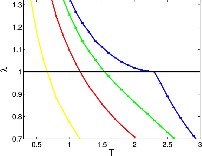
In the left part of Fig. 5 we have plotted the stability parameter as function of for different values of . One finds that is, for all values of , a monotonically decreasing function of temperature and crosses the line at exactly one point. The collection of these points defines the AT-line shown in the right part of Fig. 5 for three values of .
Of particular interest is the value of in zero external field. In the paramagnetic region characterized by the stability parameter may be determined analytically. Using we find in this case from (47) for
| (49) |
Assuming we hence find the instability of the paramagnetic solution at . Moreover, our numerical results indicate that for all .
Because the numerics is somewhat subtle when is near to a -function we corroborate this result by a perturbative study of the eigenvalue problem to leading order in the reduced temperature . To this end we expand (47) in up to order . Using the symmetry of and the truncated eigenvalue equation acquires the form with the vector . The matrix elements depend on the moments of which to the required order in the reduced temperature read
| (50) |
where we defined
| (51) |
For the largest eigenvalue of we find
| (52) |
The coefficient of the quadratic term is always positive, since decreases with as implied by (51) and .
We therefore find for all in the Lévy spin glass. Correspondingly there is no stable replica symmetric glass phase as proposed in [9, 10]. The AT-line for the Lévy spin glass as shown in the right part of Fig. 5 looks indeed qualitatively similar to other spin-glass models.
We finally comment on the assumption made after eq. (49). For we differentiate (47) times where is the first derivative with . Evaluating this equation at in the paramagnetic region i.e. for we infer that the corresponding eigenvalue is given by
Since decreases with , it results that eigenfunctions with give rise to eigenvalues which are smaller than those for eigenfunctions with and are hence not relevant for the stability problem at hand.

VI One-step RSB
The RS solution fails at low temperatures as it ignores the possibility of several pure states [20]. We therefore consider a solution which takes into account the existence of many pure states and corresponds to the one-step RSB solution in the replica formalism. The local fields corresponding to the different states are assumed to be independent random variables sampled from a site dependent distribution . After averaging over the disorder, the natural order parameter is the probability distribution of the local field distributions , and one can derive a self-consistent equation for it. In this section we work at zero temperature, where RSB effects should be most pronounced, and we show how to compute the ground-state energy density of the model within the one-step RSB. For simplicity we shall keep to the case of zero external field. The method which we use to derive expressions for the ground-state energy consists in using the truncated model, to which the general one-step RSB approach to diluted models developed in [24] can be applied. The limit is performed analytically at the end of the calculations. We shall derive the complete one-step RSB equations and solve them numerically using an approximation called the factorized approximation [25].
The assumption of one-step RSB is the following: for a fixed realization of the disorder the local fields on a given site are random variables due to the existence of many local ground states. We denote by the corresponding site dependent probability distribution.
When iterating, i.e. merging spins at a new site, the update rule for the probability distribution at this new site reads
| (53) |
where is the one-step RSB parameter, the constant ensures the normalization of , and is the zero temperature limit of (5) . (Notice that we use a slightly different notation from the one in [24]: we consider the update rules for the probability distributions , instead of used in [24]; this is to ensure a safe limit).
The ground-state energy of the Lévy spin glass is obtained within the one-step RSB approximation by maximizing
| (54) |
with respect to , where the energy shifts and are given below.
The energy shift corresponding to a site addition reads
| (55) | |||||
where denotes the distribution of the fields acting on the new spin connected to old ones.
The energy shift due to a bond addition amounts to
| (56) | |||||
After the average over disorder, the added site has the same properties as the old ones, and a self-consistency equation for the order parameter can be derived: in (53) must have the same distribution as the . Assuming that is also from the same distribution (which is the case in the limit) the averaged energy shifts read
| (57) |
and
| (58) |
respectively, where denotes an average in which is drawn from the probability distribution .
We have now all ingredients entering of the truncated model and the limit can be performed to obtain the corresponding expression for the Lévy spin glass. The symmetry of the averaged field distributions is crucial in this case as
| (59) |
leads to a convergent integral in (58) at small values of . One obtains
Notice that the self-consistent equation for the mean with respect to , denoted by , coincides, in the limits and , with the self-consistent equation (7) for the RS order parameter for zero temperature and zero external field. In particular one recovers in this limit:
| (60) |
VI.1 Factorized approximation
It is numerically rather heavy to sample from the distribution . The factorized approximation makes the task much easier by confining the space of all distributions to one distribution , i.e. it assumes that is a functional delta-function. Within this ansatz a population dynamics algorithm can be easily applied to determine for all values of the parameter . One then has to find the maximum of the function
| (61) |
where denotes
An expansion of at small and large values of allows to perform the integral in (61) analytically in the corresponding regions. For small values of one obtains , whereas in the large limit one has
A numerical test of the result for large shows that the asymptotic behavior is reached for . Using this decomposition, the computation of becomes numerically easy. We have obtained the distribution by a population dynamics algorithm after performing iterations for a population of fields. The result is shown in Fig. 6, which plots the relative increase compared to the RS solution as a function of the one-step RSB parameter . The maximal value of gives the estimate for the ground state energy of the Lévy spin glass within the one-step RSB factorized approximation. We see that the relative corrections to this ground state energy due to RSB remain rather small, of the order of one to two per cent, which is comparable to the typical corrections found for instance in the SK model [26]. It is also smaller when is close to , which agrees with the intuition according to which a smaller value of leads to a stronger hierarchy of couplings and therefore to a lesser degree of frustration.

VII Conclusion
We have presented a detailed study of the properties of the Lévy spin glass at the replica symmetric level at all temperatures and magnetic fields, and a one-step RSB study at zero temperature and zero external field. One main ingredient of this study has been the introduction of a truncated model where the couplings with values smaller than a cutoff are neglected. The truncated model naturally enters the category of dilute spin glasses for which various techniques have been developed in recent years, allowing for a detailed analysis. The limit requires some care, and complicates notably the analysis with respect to the studies of ’usual’ spin glasses, but we have shown that it can be controlled.
The physical picture which has been obtained shows a spin glass behavior which is generally much closer to the standard behavior found in the SK or in diluted models than what had been claimed before. Within the RS approximation, the entropy decreases with temperature and becomes negative at low temperatures, but does not turn back to when . The AT instability line can be computed, and the whole spin glass phase turns out to be unstable with respect to RSB effects. On the other hand, the quantitative effects of RSB on the ground state energy are relatively small and become smaller with decreasing the Lévy exponent .
Acknowledgements.
We would like to thank Jean-Philippe Bouchaud, Helmut Katzgraber, and Martin Weigt for interesting discussions. Financial support from the Deutsche Forschungsgemeinschaft under EN 278/7 is gratefully acknowledged. MM thanks the Alexander von Humboldt foundation for its support.References
- [1] Edwards S. F. and Anderson P. W., J. Phys. F5, 965 (1975)
- [2] Binder K. and Young A. P. Rev. Mod. Phys. 58, 801 (1986)
- [3] Mézard M., Parisi G., and Virasoro M. A., Spin-glass Theory and Beyond (World Scientific, Singapore, 1987)
- [4] Gnedenko B. V. and Kolmogorov A. N., Limit Distributions for Sums of Independent Random Variables (Addison-Wesley, Reading MA, 1954)
- [5] Klein M. W. and Brout R. Phys. Rev. 132, 2412 (1963)
- [6] Klein M. W., Phys. Rev. 173, 552 (1968)
- [7] Newman C. M. and Stein D. L., Phys. Rev. Lett. 72, 2286 (1994)
- [8] Cieplak M., Maritan A., and Banavar J. R., Phys. Rev. Lett. 72, 2320 (1994)
- [9] Cizeau P. and Bouchaud J.-P., J. Phys. A26, L187 (1993)
- [10] Cizeau P., Evenements rares et systemes desordonnes, PhD-thesis, Paris, 1994
- [11] de Almeida J. R. L. and Thouless D. J., J. Phys. A11, 983 (1978)
- [12] Janzen K., Hartmann A. K., and Engel A., J. Stat. Mech., P04006 (2008) a slightly modified choice of the coupling distribution is used
- [13] Neri I., Metz F. L., and Bollé D., J. Stat. Mech., P01010 (2010)
- [14] Janzen K., Engel A., and Mézard M., EPL 89, 67002 (2010)
- [15] Sherrington D. and Kirkpatrick S., Phys. Rev. Lett. 35, 1972 (1975)
- [16] Viana L. and Bray A. J., J. Phys. C18, 3037 (1985)
- [17] Kanter I. and Sompolinski H., Phys. Rev. Lett. 58, 164 (1987)
- [18] Mézard M. and Parisi G., Europhys. Lett. 3, 1067 (1987)
- [19] Raymond J. R. and Saad D., J. Phys. A41, 324014 (2008)
- [20] Mézard M. and Parisi G., Eur. Phys. J. B 20, 217 (2001)
- [21] Mézard M. and Montanari A. Information, Physics and Computation (Oxford University Press, Oxford, 2009)
- [22] Monasson R., J. Phys. A31, 513 (1998)
- [23] Weigt M. and Monasson R., Europhys. Lett. 36, 209 (1996)
- [24] Mézard M. and Parisi G.,J. Stat. Phys. 111,1 (2003)
- [25] Wong, K. Y. and Sherrington D., J. Phys. A21, L459 (1988)
- [26] Parisi G., J. Phys. A13, L115 (1980).