Unevenly-sampled signals: a general formalism of the Lomb-Scargle periodogram
Abstract
The periodogram is a popular tool that tests whether a signal consists only of noise or if it also includes other components. The main issue of this method is to define a critical detection threshold that allows identification of a component other than noise, when a peak in the periodogram exceeds it. In the case of signals sampled on a regular time grid, determination of such a threshold is relatively simple. When the sampling is uneven, however, things are more complicated. The most popular solution in this case is to use the Lomb-Scargle periodogram, but this method can be used only when the noise is the realization of a zero-mean, white (i.e. flat-spectrum) random process. In this paper, we present a general formalism based on matrix algebra, which permits analysis of the statistical properties of a periodogram independently of the characteristics of noise (e.g. colored and/or non-stationary), as well as the characteristics of sampling.
Key Words.
Methods: data analysis – Methods: statistical1 Introduction
Spectral analysis is a popular tool for testing whether a given experimental time series contains only noise, i.e. , or whether some other component is present, i.e. . The classic approach is to fit the time series with the model function
| (1) |
. If, for example, a periodic component is present with a frequency close to one in the set , then the periodogram ,
| (2) |
will show a prominent peak close to . If is semi-periodic or even non-periodic, the situation is more complicated since more peaks are expected. The main problem with the use of this technique is the definition of a detection threshold that fixes the contribution of noise in such a way that, when a peak exceeds it, the presence of a component can be claimed. In the case of signals sampled on a regular time grid, the determination of such a threshold is a relatively simple procedure, but this is not the case when the condition of regularity does not apply. In this respect, several solutions have been proposed (see Lomb 1976; Ferraz-Mello 1981; Scargle 1982; Gilliland & Baliunas 1987; Reegen 2007; Zechmeister & Kürster 2009, and references therein) that, however, work only under rather restrictive conditions (e.g. white and/or stationary noise) and are difficult to extend to more general situations.
In this paper, a general formalism is presented that allows analysis of the statistical properties of periodograms independently of the specific characteristics of the noise and the sampling of the signal. In Sec. 2 the formalism is presented for the case of even sampling and its extension to arbitrary sampling in Sec. 3. The usefulness of the proposed formalism is illustrated in Sec. 4, where the case of white noise with a mean different from zero and that of colored noise is calculated. In Sec. 5 the relationship between the periodogram and the least-squares method is considered. Finally, on the basis of simulated signals and a real time series, we discuss in Sec. 6 whether the use of algorithms specifically developed for computing the periodogram of unevenly-sampled time series is really advantageous.
2 Periodogram analysis in the case of even sampling
If a continuous signal is sampled on a set of equispaced time instants , a time series , is obtained. Its discrete Fourier transform (DFT) is given by
| (3) |
with . The sequence can be recovered from by means of
| (4) |
The set provides the so-called Fourier frequencies. Implicit in the use of DFT is the assumption that is a periodic sequence with period where .
In matrix notation, Eqs. (3) and (4) can be written in the form
| (5) |
and
| (6) |
Here, and are column arrays that contain, respectively, the sequences and , and is the so-called “Fourier matrix”, which is an square, symmetric matrix whose -entry 11 1 In the following, the element in the th row and th column of an matrix will be indicated with or alternatively with , , . is given by
| (7) |
The superscript “∗” denotes the complex conjugate transpose. Matrix is unitary, i.e.,
| (8) |
with the identity matrix. Another useful property is that
| (9) |
with
| (10) |
By means of Eq. (9) it can be shown that
| (11) |
where and and where and are the real and the imaginary parts of a complex quantity. Indeed,
| (12) |
and is a real matrix, hence Eq. (11) has to hold. From Eq. (3) it is also possible to see that is a real quantity. In the case that is an even number, the same holds for where and represents the smallest integer greater than . Finally, dealing with , only half of this array can be considered, since , , where if and zero otherwise. With this notation, the periodogram of is defined as
| (13) |
where is the th entry of the array 22 2 From now on, if is an column array, then is a column array that contains the first entries of , i.e. . Similarly, if is an matrix, then is a matrix that contains the first rows of . and denotes the Euclidean norm. By means of
| (14) |
a column array obtained by the column concatenation of and , Eq. (13) can be rewritten in the form
| (15) |
In Sect. 5 it is shown that this periodogram is equivalent to that obtainable by means the least-squares fit of model (1) with , and .
An important point to stress is that, if is the realization of a (not necessarily Gaussian) random process, then each is given by the sum of random variables. This is because of the linearity of the Fourier operator . Thanks to the central limit theorem, therefore, the entries of can be expected to be Gaussian random quantities. As a consequence, the entries of can also be expected to be Gaussian random quantities with covariance matrix given by
| (16) |
Here, denotes the expectation operator, is the covariance matrix of , and the matrix obtained by the first rows of the Fourier matrix . From Eqs. (16) and (11), it is easy to deduce that, if is the realization of a standard white-noise process, i.e., , then is a diagonal matrix with , and . In other words, the entries of are mutually uncorrelated. In turn, this means that is uncorrelated with . If is a colored (not necessarily stationary) noise process, i.e. is not a diagonal matrix, then this holds also for . However, from it is possible to obtain an array containing mutually uncorrelated entries by means of the transformation
| (17) |
The matrix can be computed via
| (18) |
with the orthogonal matrix whose columns contain the eigenvectors of and a diagonal matrix containing the corresponding eigenvalues . This decomposition is particularly simple and computationally efficient if is a circulant matrix since it can be diagonalized according to
| (19) |
where “” denotes a diagonal matrix whose diagonal entries are given by the array and is the first column of . Because of this, the decomposition (18) can be directly computed with and ; hence, . This means that the whitening operation can be performed in the harmonic domain through the following procedure: a) computation of , i.e. the DFT of ; b) computation of ; and c) the inverse DFT of . A potential difficulty in using transformation (17) is that is required to be of full rank. Such a condition can be expected to be satisfied in most practical applications. Some problems can arise if the time step of the sampling is much shorter than the decorrelation time of 33 3 The decorrelation time of a random signal is the time interval such that two values and , with , can be considered as uncorrelated.. Indeed, some columns (and therefore some rows) of could almost be identical i.e., this matrix could become numerically ill-conditioned. In this case, the most natural solution consists of averaging the data that are close in time.
When the periodogram is used to test whether vs. , a threshold has to be defined such that, with a prefixed probability, a peak in that exceeds can be expected to not arise because of the noise. This requires knowledge of the statistical properties of under the hypothesis that . The simplest situation is when is the realization of a standard white-noise process. In fact, since the entries of are uncorrelated random Gaussian quantities, from Eq. (15) it can be derived that the entries of are (asymptotically) independent quantities distributed according to a distribution44 4 denotes the chi-square distribution with two degrees of freedom.. As a consequence, independent of the frequency , a threshold can be determined that corresponds to the level that a peak due to the noise would exceed with a prefixed probability when a number of (statistically independent) frequencies are inspected. More specifically, is the highest value for which (Scargle 1982), in formula
| (20) |
If the entire periodogram is inspected, then . Commonly, is called the level of false alarm.
Threshold (20) is not applicable when the noise is colored. However, the requirement to fix a different level for each frequency can be avoided if the original signal is transformed into
| (21) |
Indeed, under the hypothesis that , the entries of are uncorrelated and unit-variance random quantities. As seen above, this operation should not be difficult. Some problems emerge if the decomposition (18) is carried out by means of the efficient DFT approach described above (a necessary approach in the case of very long sequences of data). This is because, in forming , it is necessary to take the periodicity of the sequence forced by the DFT into account. In other words, it is necessary to impose a spurious correlation among the first and the last entries in . For instance, for a stationary noise process, is a Toeplitz matrix, but it has to be approximated with a circulant one. When dealing with sampled signals, this is an unavoidable problem that no technique can completely solve. A classical solution to relieving this situation is the windowing method, i.e., the substitution of in Eq. (3) with , where is some prefixed discrete function (window) that makes the signal gently reduce to zero at the extreme of the sampling interval (Oppenheim & Shafer 1989, e.g. see). This method can be expected to work satisfactorily only when the decorrelation time of noise is shorter than the length of the signal.
3 Periodogram analysis in the case of uneven sampling
If a signal is sampled on an uneven set of time instants, some problems emerge: it is no longer possible to define a set of "natural" frequencies such as those obtained by the Fourier transform. In turn, this implies some ambiguities in the definition of the Nyquist frequency that, loosely speaking, corresponds to the highest frequencies that contain information on the signal of interest (Vio et al. 2000; Koen 2006, e.g. see). As a consequence, Eq. (3) has to be modified. In the following, with no loss of generality, it is assumed that is sampled at arbitrary time instants with , and the remaining arbitrarily distributed within this interval. Moreover, a set of frequencies is considered with . Such a set corresponds to the frequencies that are typically inspected when looking for a periodicity. However, others can be chosen. With these conditions, a transformation corresponding to the one given by Eq. (5) is
| (22) |
where
| (23) |
, and is a real positive number. Because of the normalization by , time is expressed in units of the shortest sampling time interval. Apart from the substitution of the Fourier matrix with , the uneven sampling of signals does not modify the formalism introduced in the previous section. In particular, the covariance matrix defined in Eq. (16) becomes
| (24) |
The Fourier matrix does not have the properties (8)-(12). As consequence, and also in the case that is the realization of a standard white-noise process i.e. , matrix ,
| (25) |
is not diagonal. In general, is not even diagonalizable. For example, this happens when the periodogram of a time series containing data is computed on frequencies with (a typical situation in practical applications). This implies that the entries of cannot be made mutually uncorrelated. Obviously, the same holds for the entries of as given by Eq. (15). As a consequence, although a number of frequencies are considered in , at most only of them are statistically independent55 5 This is because, if , the rank of the matrix is smaller than or equal to . This implies that the array has at most degrees of freedom. Since each entry of is given by the sum of two entries of , then a periodogram has at most degrees of freedom.. Particularly troublesome is that, for a given frequency , , and (i.e. and ) are also correlated. This makes it difficult to fix the statistical characteristics of . In this respect, two choices are possible. The first consists in the determination, for each frequency, of the PDF of . Actually, this is a rather involved approach, because and have variance and , respectively, and covariance . Therefore, once and are normalized to unit variance, each is given by the sum of two correlated random quantities. Although available in analytical form (Simon 2006), the resulting PDF is rather complex and hence difficult to handle (Reegen 2007, for an alternative approach, see). Moreover, there is the additional problem that changes with . A simpler alternative is the use of two uncorrelated and unit-variance random quantities, and , obtained through the transformation
| (26) |
Here, , , is a diagonal matrix whose entries are given by the reciprocal of the square root of the non-zero eigenvalues of the covariance matrix
| (27) |
zero otherwise, and is an orthogonal matrix that contains the corresponding eigenvectors66 6 The diagonal elements and of can be trivially computed through the solution of the quadratic equation , with and denoting the trace and determinant operators. The arrays and , which constitute the columns of , can be obtained by solving the equations , .. Indeed, if the periodogram is defined as
| (28) |
then each is given by the sum of two independent, unit-variance, Gaussian random quantities. As a consequence, the corresponding PDF is, independently of , a whose cumulative distribution function (CDF) is the exponential function. This permits determining the statistical significance of for a specified frequency . Things become more complex if frequencies are inspected when looking for a peak. Indeed, also after the operation (26), it happens that for , i.e., the frequencies of the periodogram remain mutually correlated. This is an unavoidable problem. Because of it, does not correspond to the number of independent frequencies, so the level of false alarm (20) cannot be computed. However, since is the same for all the frequencies, an upper limit can be fixed for by setting . The periodogram obtained by means of Eq. (28) corresponds to the original Lomb-Scargle periodogram.
Since the transformation (17) does not depend on the characteristics of the signal sampling, the strategy of following in the case that is the realization of (not necessarily stationary) colored noise is simply the one in Sec. 2 i.e. transformation of to an array with uncorrelated entries. After that, the Lomb-Scargle periodogram can be computed. It is worth noticing that this simple result has been possible thanks to a formulation of the problem in the time domain and the use of the matrix notation. The same results could have been obtained by following the popular approach of working in the harmonic domain but at the price of a much more difficult derivation.
4 Two examples
To illustrate the usefulness and the simplicity of the proposed formalism in handling different situations from the classical ones, we show two examples in this section.
The first consists of a periodogram of a mean-subtracted time series. The evaluation of the reliability of a peak in the periodogram of a signal requires that (under the null hypothesis ) be the realization of a zero-mean noise process. In most experimental situations, this condition is not fulfilled and one works with a centered (i.e. mean-subtracted) version of . This, however, introduces some (often neglected) problems. The case where is the realization of a discrete white noise process with variance has been considered several times in the literature. An example is the paper by Zechmeister & Kürster (2009) where a rather elaborate solution is presented. With the approach proposed here, a simpler solution can be obtained if one takes into consideration that the subtraction of the mean from forces a spurious correlation among the entries of in such a way that the covariance matrix is given by
| (29) |
where is number of entries of and an matrix with every entry equal to unity. Since this matrix is singular, it cannot be diagonalized and therefore cannot be whitened. In any case, if in Eq. (24) matrix is substituted for and one sets
| (30) |
then it is a trivial matter to decorrelate and by means of Eqs. (26)-(27) and to compute the periodogram through Eq. (28). This result can be easily extend to the case where, because of measurement errors, each entry of has its own variance and a weighted mean is subtracted from the data sequence i.e. , with . Indeed, it is sufficient to substitute as given by Eq. (29) with
| (31) |
where . The rest of the procedure remains unmodified.
The second example consists of zero-mean colored noise. The improvement in the quality of the results obtainable with the approach presented in the previous section is visible in Fig. 1. The top left panel shows a discrete signal , , simulated on a regular grid of time instants but with missing data in the ranges and . Here, is the realization of a discrete, zero-mean, colored noise process whose autocovariance function is given in the top right panel. From the bottom left panel, it is evident that Lomb-Scargle periodogram of the original sequence provides rather ambiguous results concerning the presence of a sinusoidal component. On the other hand, such component is well visible in the bottom right panel that shows the Lomb-Scargle periodogram of the sequence .
5 Periodogram and least-squares fit of sinusoids
The formalism proposed here is also useful in the context of more theoretical questions (but with important practical implications). For example, a point often overlooked in the astronomical literature is the relationship between the periodogram and the least-squares fit of sine functions. Often these two methods are believed to be equivalent. Actually, this is true only when the sampling is regular and the frequencies of the sinusoids are given by the Fourier ones. Indeed, if and , , then Eq. (1) can be written in the form
| (32) |
with
| (33) |
and . The least-squares solution of system (32) is given by
| (34) |
where “+” denotes Moore-Penrose pseudo-inverse (Björck 1996). In the case of even sampling, i.e. when and , it happens that
| (35) |
In other words, coefficients and , as given by the least-squares approach, can be obtained through the DFT of , because, as shown by means of Eqs. (11), . In the case of uneven sampling, this identity is not fulfilled. Any kind of periodogram computed through Eq. (22) and the least-squares fit of sine functions has to be expected to give different results. Moreover, as only under the two above-mentioned conditions do the sine functions constitute an orthonormal basis, the least-squares fit of a single sine function per time does not in general provide the same result as the simultaneous fit of all the sinusoids as in Eq. (34) (e.g. see Hamming 1973, page 450). In particular, if an unevenly-sampled signal is given by the contribution of two or more sinusoids, the one-at-a-time fit of a single sine function provides biased results. This also holds for the Lomb-Scargle periodogram, which is equivalent to the least-squares fit of a single sinusoid with a specified frequency, with the constraint that the corresponding coefficients “” and “” are uncorrelated (Scargle 1982; Zechmeister & Kürster 2009).
6 Discussion
As demonstrated in Sec. 3, when noise has arbitrary statistical characteristics, the computation of the periodogram of an unevenly-sampled signal requires two steps:
- •
Whitening and standardization of the noise component (in this way a signal is obtained);
- •
Computation of the Lomb-Scargle periodogram of .
The first step, unavoidable even in the case of regular sampling, is a computationally expensive operation. Therefore, for time series containing more than a few thousand data points, dedicated algorithms exploiting the specific structure of (e.g. often this matrix is of banded type) have to be developed for implementing Eq. (21). However, this problem is beyond the aim of the present paper. The second step is much less time consuming. Indeed, in the case of time series containing some thousands of points and when the periodogram has to be computed on a similar number of frequencies, the direct implementation of Eqs. (22)-(28) results in a few seconds of computation time only. In other words, in many practical situations, no dedicated algorithm is really necessary. However, fast algorithms have been proposed for very long time series (Press et al. 1992).
The last issue that has to be considered is to which extent the use of the Lomb-Scargle periodogram is really advantageous. Indeed, the action of the algorithms dealing with uneven sampling is essentially directed, for each frequency , to force to be the sum of two independent Gaussian random quantities. However, although not clearly emphasized, it has already been pointed out that this operation is not critical (Scargle 1982, e.g. see). It can be expected that a periodogram computed simply through
| (36) |
with , is often very close to the one given by Eq. (28). A rigorous demonstration of this fact is difficult because of its strict dependence on the specific sampling. However, with the help of some numerical experiments and of the formalism introduced here, some insights are possible. In particular, we consider the covariance matrix of a white noise signal when sampled on different uneven time grids.
6.1 Numerical simulations
In our simulations, we take the realization of a zero-mean, unit-variance, Gaussian white-noise process sampled on time regularly-spaced instants, but with missing data (i.e. ). The available signal can be written in the form
| (37) | ||||
| (38) |
where and is an array whose entries are equal to one in correspondence to a value of that is available and zero otherwise. In this case, Eq. (3) can be written as
| (39) | ||||
| (40) |
with . Three different cases have been considered where the missing data have time indices in the ranges a) , b) and , c) , and , whereas they are randomly distributed in a fourth case . The related covariance matrices , computed through Eq. (25) with , are shown in Fig. 2, whereas Fig. 3 displays the corresponding main diagonal of the blocks and . Especially from Fig. 3 it is evident that, for an arbitrary frequency , the covariance between and is quite close to zero. This means that each entry of , as given by Eq. (36), can be assumed to be distributed according to a . From Fig. 2 it is also evident that, in the case of gaps present in the sampling pattern, there are nearby frequencies and for which not only and are mutually correlated, but also with and with . These correlations, especially those between the real and the imaginary components, disappear in the case of random sampling.
6.2 Interpretation of the results of the simulations
To understand these results, it is necessary to take into account that Eq. (39) can be rewritten in the form
| (41) | ||||
| (42) |
As is a (singular) diagonal matrix, is a (singular) circulant matrix. This implies that is given by the circular convolution of (the DFT of the original signal, inclusive of the missing data) with the spectral window (the DFT of the sampling pattern). Since for two arbitrary frequencies, say and , , , , and are mutually independent, any correlation existing between , , , and is induced by the correlation between the entries of and . Now, as shown in Fig. 4, in the presence of gaps the real and the imaginary parts of are both only significantly different from zero in a narrow interval of frequencies surrounding the origin, i.e., corresponding to the lowest frequencies ( can be interpreted as low-pass filter). This produces the correlations observed among , , and for nearby frequencies and . On the other hand, in the case of random sampling mimics the behaviour of white noise, making the correlations less important. Moreover, Fig. 5 shows that, in the case of sampling with gaps, the cross-correlation between with is significant but not centered at zero lag. This explains why the quantities and , can be strongly correlated in spite of the small correlation between and . Similar arguments also hold for the case of sampling with periodic gaps (rather common in astronomical experiments). Indeed, in practical applications the period of these gaps is somewhat smaller than the mean sampling time step of an uninterrupted sequence of data. As a consequence, both and present a sharp and narrow peak in correspondence to a frequency close to the origin. Actually, the spectral window of a sampling with periodic gaps is also characterized by the presence of aliases. However, these aliases too are sharp and narrow, and their importance decreases for increasing frequencies. The combination of these facts leads again to the quantities , , , and almost being uncorrelated if the frequencies and are not sufficiently close enough. Moreover, since with periodic gaps the cross-correlation between with can also be significant, but not centered on zero lag, then for each frequency the correlation between and is negligible. These considerations are confirmed by Figs. 6 and 7. Figure 6 displays the covariance matrix , computed through Eq. (25), of a discrete zero-mean, unit-variance, and white-noise process sampled on time instants randomly distributed (i.e. not rebinned) along six cycles (i.e. points per cycle) of the sampling pattern shown in the bottom panel of Fig. 7; frequencies have been considered. The top panel of Fig. 7 displays the main diagonal of the blocks and .
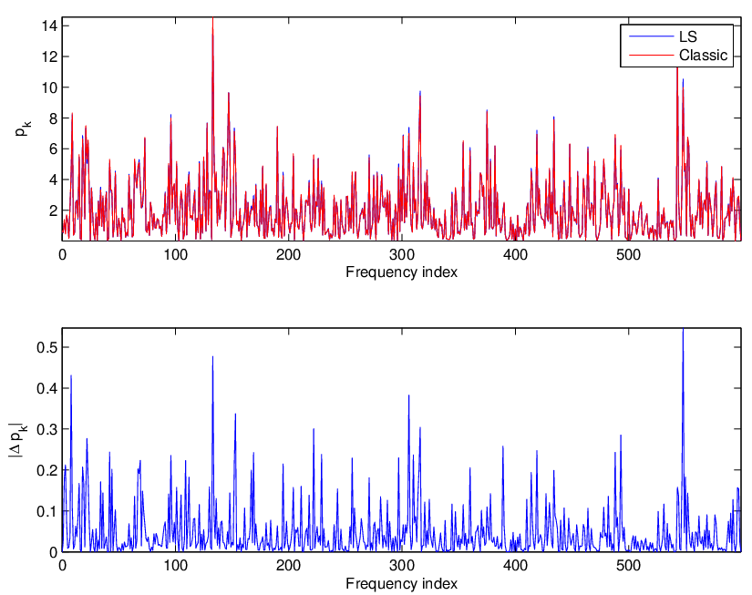
The numerical simulations indicate that the consequences of unevenly-sampled data seem to concern the number of independent frequencies in rather than the correlation between and its imaginary counterpart . At present, no general method has been developed to deal with this problem. However, it has been pointed out in the literature that the number of independent frequencies is not a critical parameter to test the significance level of a peak in . In particular, empirical arguments indicate that this number can be safely set to (Press et al. 1992, e.g. see). The conclusion is that forcing each entry of to be the sum of two independent Gaussian quantities only has minor effects. This is shown by Fig. 8 where the top panel shows that the Lomb-Scargle periodogram of the time series with periodic gaps considered above is quite similar to that provided simply by with . This is evident in the bottom panel of the same figure where the similarity of the two periodiograms is demonstrated by their absolute difference.
A final point to underline, which has important practical implications, is that for long time series the small differences visible in Fig. 8 should decrease. Indeed, as seen above, will be significantly correlated with only if the two frequencies and are close enough. The only exception is represented by the frequencies at the extremes of the frequency domain where the assumption of periodic signal intrinsic to DFT forces a spurious correlation. For longer and longer time series, this spurious correlation will affect a smaller and smaller fraction of frequencies and, as consequence, a larger and larger fraction of them will be mutually independent. This is shown in Fig. 9 where, in the context of the previous experiment, the mean absolute difference between the two periodograms is plotted as a function of , the number of cyclic sampling patterns ( in Fig. 8). This argument also explains why in many practical situations the number of independent frequencies can be safely fixed to . In conclusion, only in the case of signals that contain a small number of data, the Lomb-Scargle periodogram can be expected to exhibit noticeable differences from the periodogram given by Eq. (36). Often, using it does not change anything. Comparable results can be expected with less sophisticated approaches.
6.3 Application to an astronomical time series
As an example of an unsophisticated method able to produce results similar to those obtainable with the Lomb-Scargle periodogram, we consider the rebinning of the original time series on an arbitrarily dense regular time grid (in this way a signal with a regular sampling is obtained but some data are missing) followed by applying any of the fast Fourier transform (FFT) algorithms available nowadays. Figure 10 shows an experimental (mean-subtracted) time series versus its rebinned version. This time series, which is characterized by rather irregular sampling, was obtained with the VLA array (Biggs et al. 1999) and consists of polarisation position angle measurements at an observing frequency of 15 GHz for one of the images of the double gravitational lens system B0218+357. The original sequence contains only data and it is rebinned on a regular grid of time instants. In spite of this, as visible in Fig. 11, the corresponding periodograms, computed on equispaced frequencies by means of the Lomb-Scargle and the FFT approach, are remarkably similar. Here, the highest frequency approximately corresponds to the Nyquist frequency that is related to the shortest sampling time step. The main conclusion of this example is to point out that, although in the previous section we stated that use of the Lomb-Scargle periodogram can be expected to be effective only for time series that contain a small number of data, this is not a sufficient condition to guarantee that the method is truly useful.
7 Conclusions
In this paper we worked out a general formalism, based on the matrix algebra, that is tailored to analysis of the statistical properties of the Lomb-Scargle periodogram independently of the characteristics of the noise and the sampling. With this formalism it has become possible to develop a test for the presence of components of interest in a signal in more general situations than those considered in the current literature (e.g. when noise is colored and/or non-stationary). Moreover, we were able to clarify the relationship between the Lomb-Scargle periodogram and other techniques (e.g. the least-squares fit of sinusoids) and to fix the conditions under which the use of such method can be expected to be effective.
References
- Biggs et al. (1999) Biggs, A.D., Browne, I.W.A., Helbig, P., Koopmans, L. V. E, Wilkinson, P. N., Perley, R. A. 1999 MNRAS, 304, 349
- Björck (1996) Björck A. 1996, Numerical Methods for Least Squares Problems (Philadelphia: SIAM)
- Ferraz-Mello (1981) Ferraz-Mello, S. 1981, AJ, 86, 619
- Gilliland & Baliunas (1987) Gilliland, R.L., & Baliunas, S.L. 1987, ApJ, 314, 766
- Koen (2006) Koen, C. 2006, MNRAS, 37, 1390
- Hamming (1973) Hamming, R.W. 1973, Numerical Methods For Scientists and Engineering (New York: Dover)
- Lomb (1976) Lomb 1976, Ap&SS, 39, 447
- Oppenheim & Shafer (1989) Oppenhaim, A.V., & Shafer, R.W. 1989, Discrete-time Signal Processing, (London: Prentice Hall)
- Press et al. (1992) Press, W.H., Teukolsky, S.A., Vetterling, W.T., & Flannery, B.P. 1992, Numerical Recipes (Cambridge: Cambridge University Press)
- Reegen (2007) Reegen, P. 2007, A&A, 467, 1353
- Scargle (1982) Scargle, J.D. 1982, ApJ, 263, 835
- Simon (2006) Simon, M.K. 2006, Probability Distributions Involving Gaussian Random Variables (Heidelberg: Springer)
- Vio et al. (2000) Vio, R., Strohmer, T. & Wamsteker, W. 2000, PASP, 112, 74
- Zechmeister & Kürster (2009) Zechmeister, M., & Kürster, M. 2009, A&A, 496, 577