Fractal boundary basins in spherically symmetric theory
Abstract
Results are presented from numerical simulations of the flat-space nonlinear Klein-Gordon equation with an asymmetric double-well potential in spherical symmetry. Exit criteria are defined for the simulations that are used to help understand the boundaries of the basins of attraction for Gaussian “bubble” initial data. The first exit criteria, based on the immediate collapse or expansion of bubble radius, is used to observe the departure of the scalar field from a static intermediate attractor solution. The boundary separating these two behaviors in parameter space is smooth and demonstrates a time-scaling law with an exponent that depends on the asymmetry of the potential. The second exit criteria differentiates between the creation of an expanding true-vacuum bubble and dispersion of the field leaving the false vacuum; the boundary separating these basins of attraction is shown to demonstrate fractal behavior. The basins are defined by the number of bounces that the field undergoes before inducing a phase transition. A third, hybrid exit criteria is used to determine the location of the boundary to arbitrary precision and to characterize the threshold behavior. The possible effects this behavior might have on cosmological phase transitions are briefly discussed.
pacs
04.25.D-,11.27.+d,95.10.Fh,98.80.CqI Introduction
While expanding and collapsing scalar field bubbles have each been given a great deal of attention in the physics community (largely in the contexts of phase transitions and oscillons, respectively), there is surprisingly little focus on the solutions that live on the threshold of those two end states. This paper focuses on the critical phenomena that exist near this threshold and the fractal boundaries that define it.
The model used in this paper is the nonlinear Klein-Gordon (nlKG) equation with an asymmetric double-well potential (ADWP). The ADWP used here is the typical quartic potential with two stable minima: one global minimum at the lowest possible potential energy (the “true” vacuum) and one local minimum at a higher energy (the “false” vacuum). In the study of phase transitions, one typically considers initial data that consist of perturbations on top of the false vacuum. If the perturbations are large enough, the tendency for the field to transition to the energetically more favorable true vacuum can overcome the effective “surface tension” that would cause the bubble to collapse. When that is the case, the bubble wall will expand outward causing a transition from the false to the true vacuum; the resulting solution is referred to as a supercritical bubble. If the perturbations are small, however, a phase transition will not occur; the scalar field will collapse and eventually disperse, and the solution is referred to as a subcritical bubble.
When the nlKG equation was first studied in the context of phase transitions, research efforts focused largely on supercritical bubbles, and in particular, on domain walls. Subcritical bubbles tended to be neglected because, by definition, they do not induce a phase transition; it was not understood until much later that subcritical bubbles could still have cosmological implications. For a wide range of initial data leading to subcritical bubbles, there exist localized oscillating solutions, called oscillons, that have lifetimes that are large compared to naive expectations. Oscillons were originally discovered by Bogolubsky and Makhankov [1] and have been thoroughly investigated by numerous authors using many types of nonlinear models [2, 3, 4, 5, 6, 7, 8, 9, 10, 11, 12]; the effect oscillons may have on phase transitions has been of great interest [13, 14, 15]. The work by Gleiser and Sicilia [16] is an excellent summary and analytic characterization of the salient features of oscillons.
While most of the simulations presented in this paper result in the formation of either an oscillon or a domain wall, this paper actually focuses on neither; this paper focuses on the nonlinear dynamics that exist on the threshold of creating one of these two end states. This paper begins with a presentation of general formalism and definitions in Section II. In Section III, methods are presented that can be used to solve for the intermediate attractor solutions to the nlKG-ADWP system. It is shown that in the neighborhood of the attractor, Type I critical phenomena similar to those observed in gravitational collapse are present. Section IV demonstrates that the basin boundaries have fractal structure and can be parameterized by the number of times they “bounce” before inducing a phase transition, not unlike the kink/antikink soliton (domain wall) collisions of [17]. Furthermore, methods are presented that allow for the arbitrarily precise determination of the location of the fractal edges. Being able to explore these edges in parameter space reveals that both a static intermediate attractor solution and Type I critical phenomena appear to exist on every basin boundary. Finally, Appendix A presents a rough approximation for the Minkowski-Bouligand fractal dimension of a data set with the basic properties observed in the nlKG-ADWP system.
II General Formalism and Definitions
The nlKG action is
| (1) |
where and is the flat spacetime metric on a four-dimensional manifold. The potential is given by , where is a measure of the asymmetry of the potential. When , is a symmetric double-well potential with vacuum states at and . With , the false and true vacuums are and , respectively.
Variation of the action with respect to gives the covariant equation of motion
| (2) |
which after imposing spherical symmetry and using spherical coordinates (,) gives
| (3) | |||||
| (4) | |||||
| (5) |
where and . The spacetime admits a timelike Killing vector that gives rise to the conserved energy
| (6) |
where is the radius of the outer boundary, and the constant is subtracted to give for (i.e., everywhere at the true vacuum).
The initial data used to evolve (3), (4), and (5) are taken to be a simple Gaussian bubble:
| (7) |
This bubble type of initial data interpolates between the true and false vacuums and represents a perturbation away from the false vacuum that may (or may not) lead to a phase transition.
To explore the dynamics of the scalar field bubbles, it is useful to define an ancillary function
| (8) |
where , and satisfies at if for some . More simply put, is the maximum radius for which the field is halfway between the true and false vacuums, and zero if at time the field does not anywhere equal . For example, using the initial data profile (7) and the definition (8), one can define , which is simply the radius (at half-maximum) of the Gaussian profile, . For supercritical bubbles, is a reasonable approximation to the location of the bubble wall.
For collapsing bubbles, the number of oscillations, or bounces, of , denoted , is defined to be the number of times
| (9) |
for any . To retain common terminology with the works on kink/antikink soliton collisions, the term “bounce” will be used to describe the oscillations the field undergoes.
Finally, all solutions to (3), (4), and (5) are obtained using a second-order iterative Crank-Nicholson finite difference scheme with higher-order Kreiss-Oliger dissipation [2]. A simple outgoing boundary condition is used at the exterior of the grid, but the grid is chosen to be large enough such that any reflected radiation could not travel back to origin during the evolution. Since this work is focused on the threshold of bubble expansion and not the long-term behavior of oscillons, this approach is simple and effective.
III The intermediate attractor
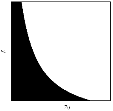
It has been shown in [18] that solutions to (3), (4), and (5) obey a time-scaling law near the threshold of expansion or collapse. The exit criteria for the simulations in [18] is based on the bubble radius moving sufficiently far away from the initial bubble radius, :
| (10) |
where and are constants chosen to be above and below , respectively. Figure 1 displays the end state (expansion or collapse) as a function of the width of the initial bubble and the asymmetry parameter . The boundary between the two end states is observed to be smooth, and the -dependent threshold value of is defined to be , or just .
III.1 Time-scaling law
To explore the properties of the threshold, one must find precisely. This is done by fixing the asymmetry parameter and varying . The search begins with a that is known to expand and a that is known to collapse. Evolutions are run with test values that successively bisect and until machine precision is reached (64-bit double-precision variables used). For a fixed asymmetry parameter , one can observe the lifetime of the solution as a function of . The solution lifetimes are observed to obey a time-scaling law
| (11) |
with an exponent that depends on .
The time-scaling law can be observed on both the expansion and collapse sides of in Fig. 2.
The time scaling laws like (11) are not uncommon in the study of nonlinear field theories. Similar Type I critical phenomena are observed in the gravitational collapse of a wide range of matter fields [19, 20, 21, 22, 23, 24, 25]. In these models, in the limit that approaches , the solutions each approach an unstable intermediate attractor solution with Lyapunov exponent . While the exact nature of the intermediate attractor solutions varies depending on the physical model, the most common attractor type is static [23, 22, 24, 21].
III.2 The nlKG static intermediate attractor
Not surprisingly, observation of the threshold dynamic solutions shows that the field appears to consist of small oscillations on top of an underlying static solution. Fig. 3 shows snapshots of a near-critical evolution for values of slightly above and below .
Guided by this observation and other examples of Type I critical phenomena, a static solution to (3), (4), and (5) is obtained by invoking a static ansatz (setting all time derivatives equal to zero). The static field equations are
| (12) | |||||
| (13) |
and are solved by “shooting.”
The solution of (12) and (13) is very similar to the one-dimensional particle subject to a potential of , differing only by the geometric factor in the spatial Laplacian and the exchange of and . The critical solution is obtained by solving (12) and (13) with and different initial values of . The solutions have three types of behavior as : or oscillation in the local minimum of . Bisecting on the threshold of the end state and the oscillation end state yields the desired critical solution that asymptotically approaches the false vacuum. In the one-dimensional particle analogy, this is like finding the perfect initial position of the particle so it can “roll” through the trough of the potential and come to a perfect stop at the unstable minimum at (Fig. 4 inset). Fig. 4 shows the fine-tuned solution to (12) and (13) for .
In addition to showing the evolution of the dynamic solutions, Fig. 3 also shows the static intermediate attractor solution. It appears that the threshold solution is a superposition of the static solution and a small amplitude time-dependent localized “shape mode,” reminiscent of one-dimensional kink/antikink soliton collisions [26]. Fig. 5 shows the approximate bubble radius, , for the same two near-critical solutions shown in Fig. 3; it can be clearly seen that the bubble radius for the dynamic solutions oscillates about the bubble radius of the static intermediate attractor before collapsing or expanding.
IV True/False vacuum boundaries
In the previous section it was shown that divides the - parameter space into regions of immediate expansion or collapse. This section focuses on the more physical concern of what vacuum state the spacetime approaches in the limit. In regions where the bubbles expand, , the bubble wall expands outward indefinitely and induces a phase transition to the true vacuum. In regions where the bubbles collapse, however, terminates the evolution immediately after drops below , and as such, no conclusion can be drawn about which vacuum state the field will occupy as . There are three long-term behaviors observed in the collapsing field configurations: solutions that immediately disperse to leave the false vacuum, solutions that form oscillons that eventualy disperse to leave the false vacuum, and solutions that collapse but bounce back and lead to an expanding true-vacuum bubble.


An exit criteria that effectively determines which vacuum state the solution will approach as is
| (14) |
where PT and NPT refer to phase transition and no phase transition, respectively; is again the radius beyond which the bubble is assumed to induce a phase transition; is the number of bounces before assuming the solution enters the oscillon state; and is a time at which the bubble is assumed not to induce a phase transition (if has remained less than ).
Figure 6 displays three solutions subject to criteria , each exiting due to a different condition (denoted A, B, and C in the figure). Solution A is an example of a typical runaway PT solution; these solutions are easily detected with the condition and a reasonably chosen -dependent . Solution B is an example of a solution that settles into the oscillon regime, staying localized for many periods before eventually dispersing (NPT); these solutions are detected with the condition. The vast majority of the solutions discussed in this paper are of these two types (A or B). The condition is added to the NPT criteria for the cases like solution C, where the initial data perturbations are so small that the field immediately disperses without enough energy to even form an oscillon.
Figure 7 shows a bitmap displaying the PT/NPT end state as a function of and for solutions subject to . A remarkable difference can be seen when compared to Fig. 1. The simple boundary between collapsing and expanding solutions is replaced by a much more complicated fractal boundary. The extra structure is a result of solutions that bounce back after collapse to form expanding true-vacuum bubbles (see Fig. 8). These solutions collapse initially yet still lead to phase transitions. The solutions shown in Fig. 7 are shaded (colored online) differently based on the number of times they bounce before expanding to induce a phase transition. Each band of bounces is immediately surrounded by a set of bands of bounces that approach it from both sides in -space. The structure appears to be fractal given it continues to repeat itself in a self-similar fashion upon successive magnification. This structure closely resembles the structure observed in [17], except that instead of colliding domain walls (kink/antikink soliton collisions) parameterized by boost velocity, it arises from collapsing bubbles parameterized by initial bubble radius.
The width of -space surrounding that demonstrates this fractal bounce behavior is defined to be ; given this, the region of -space demonstrating this behavior is given by
| (15) |
In Fig. 7, it is observed that for , and .
IV.1 Threshold of the -bounce band
After observing the fractal structure of the PT/NPT boundaries in Fig. 7, one might wonder whether there exist scaling laws at the threshold of each boundary, and if so, whether the scaling law exponents and intermediate attractor solutions are universal. To answer this question, one must be able to determine the boundary of a given -bounce band to arbitrary precision. One might attempt to use the same bisecting technique used in Section III.1 but with the PT/NPT condition . Unfortunately, this technique fails due to the fractal nature of the boundary. For a fixed , one cannot use to find a (PT end state) and a (NPT end state) that bound a single PT/NPT boundary. In fact, it appears that there would be an infinite number of such boundaries. Any bisecting approach using that began with a in the desired PT band and a outside the band would almost definitely lead to hopping to a different band.
However, one can find the boundary of an -bounce band if one exploits the fact that an -bounce band is approached by either NPT solutions that form oscillons or PT solutions with more than bounces. If one starts with a that is in the -bounce band and a that is sufficiently close but not in the band, the hybrid condition
| (16) |
will successfully find the desired edge, denoted , where Solutions inside the -bounce band will induce a phase transition and exit due to the condition. Solutions outside the -bounce band will bounce more than times since they either form an oscillon or are contained in a PT band with more than bounces; when these solutions bounce more than times, they exit as what is here referred to as a delayed-collapse solution.
To understand the nature of solutions near the fractal boundary, solutions are first evolved with exit criteria in order to find . Then, solutions are obtained with exit criteria using that approach from either side, so that one can observe the PT or NPT end state of the solutions near . Fig. 9 demonstrates the time-scaling law
| (17) |
for approaching on the PT side. While similar to the time-scaling seen in Section III.1, there now appears to be a scaling law observed on each of the infinitely many PT/NPT boundaries. Furthermore, the exponent appears to be universal for a given .
Fig. 10 shows a mix of PT and NPT solutions for approaching from the delayed-collapse side. The figure seems to imply that each band of PT solutions with bounces is approached by an infinite number of PT bands of bounces. For example, in the plot in Fig. 10, each of the curves represent PT solutions with bounces. The main dips that can be seen are for PT solutions with bounces; the regions of fine structure seen around the bands each have bounces, showing that the structure continues at finer and finer scales. The gaps between the bands are for that form oscillons and eventually disperse (with no phase transition). While the appearance of the bands might only be a truncated fractal structure, the fact that the bands appear in roughly log-periodic windows that approach to machine precision highly suggests that the bands would continue ad infinitum (Appendix A discusses approximations to the fractal dimension). The time-scaling law is present yet again (with the same -dependent ) but here serves as a lower-limit envelope on the lifetime.
Finally, looking at Fig. 11 (animations online, [EPAPS_REFERENCE]) one can see that solutions on this fractal boundary indeed approach the -dependent static intermediate attractor. This strongly suggests that the solution obtained from the static ansatz (for a given ) serves as a universal intermediate attractor on the threshold of inducing a phase transition. While the fractal structure itself is not surprising given the previous understanding of kink/antikink soliton collisions [17], observing this structure in bubble collapse, the direct measuring of the time scaling law, the ability to determine the fractal boundary to arbitrary precision, and the realization that the static solution to (12) and (13) serves as an intermediate attractor on the fractal boundary all offer new insight into a classic nonlinear system.
V Discussion and Conclusions
It has been shown that the boundary between the basins of attraction for the nlKG-ADWP system (the true- and false-vacuum states) is fractal in nature. The fractal structure arises from solutions that collapse, bounce a number of times, and then expand to induce a phase transition. The solutions that induce a phase transition are organized into bands that are grouped by the number of bounces they undergo before becoming expanding bubbles. These bands form a regular and predictable (as opposed to chaotic) fractal structure in the parameter space. Bands of solutions with bounces are surrounded by bands of solutions with bounces. When viewed in -space, the roughly equal-width -bounce bands appear to approach the edges of the -bounce bands in a log-periodic fashion. A time-scaling law is observed at each fractal boundary with an exponent that depends on the asymmetry parameter , and the solutions that exist on these boundaries are shown to approach the same static intermediate attractor solution.
While the phenomena discussed here have been studied in the context of isolated scalar field collapse, one may wonder what possible impact these phenomena would have on global phase transitions induced by bubble nucleation. The Gaussian bubbles (7) are assumed to represent perturbations away from a false vacuum. For a global phase transition to occur, supercritical perturbations need to form expanding bubbles that combine, thereby inducing a global transition to the true vacuum. The impact the fractal behavior discussed in this paper might actually have on bubble nucleation would depend not only on how close to threshold these perturbations are for a given system, but also on how those perturbations vary throughout space. For example, if typical perturbations are near the threshold of expansion/collapse, , but the variation in in different perturbations throughout space is large, , the probability that these effects will have an impact on previously explored bubble nucleation rates will be low since most are not contained in and therefore do not demonstrate the fractal bounce behavior. However, if , then most are in , and the phenomena observed in this paper would likely have a significant impact on bubble nucleation rates. In this condition, one might want a way to approximate the probability that a given perturbation (given by ) would end up in either the true- or false-vacuum state; one very natural measure of this probability is related to the fractal dimension itself, which is discussed in Appendix A. Furthermore, one would not need a stochastic description of perturbations to create a phase transition that appears chaotic or random; a smoothly varying distribution of perturbations, where , would still likely create a system with a rich and complex structure.
Appendix A Minkowski-Bouligand dimension of log-periodic line segments
The structure observed in Fig. 7 seems to be fractal since a self-similar banded structure appears at successive scales of magnification. For each -bounce band, there appear to be an infinite number of –bounce bands of roughly equal width in -space that approach the -bounce band on either side of -space in a log-periodic fashion. By defining a set on that demonstrates similar behaviors, this appendix calculates an approximation to the fractal dimension of the PT/NPT boundary discussed in this paper.
The notion of dimensionality used here is the Minkowski-Bouligand, or box-counting, dimension,
| (18) |
where is the number of boxes of side length required to cover the set of PT solutions. In calculating , one can start with a single box covering the region in question. One then successively breaks the box into smaller boxes. The boxes that cover the set contribute to , and the dimension is obtained in the limit . After fixing , the - boxes reduce to line segments parameterized by . Choosing a box that is in the bulk of a PT band yields , since every box contains PT solutions and is in the set, no matter how many times it is divided into smaller boxes. Choosing a box that is far away from a PT band and in a clearly NPT region has , since no smaller box ever contains a PT solution allowing it to belong to the set. The intermediate region is a different story entirely.
Figure 12 demonstrates the two observed properties of the PT solutions. The first property is that the bands of PT solutions appear to be roughly equal width in -space, here denoted . The second property is that the bands of PT solutions appear to be an equal distance, , apart in -space. The ratio is essentially a duty cycle quantifying what proportion of the space is in the set of PT solutions. It is this observation that would allow one with limited measurements of and to approximate the fractal dimension of the system; these numbers could be used to determine the probability that any will induce a phase transition. Figure 13 shows the Minkowski-Bouligand dimension for different values of as a function of . As expected, all solutions have for since those sets are empty. Likewise, all solutions have for since those sets are completely solid lines.
The approximation discussed here is only a very rough approximation to the fractal dimension observed in the nlKG-ADWP dynamical system since it only considers a single level of recursion of the self-similar pattern. In the actual nlKG-ADWP system, in addition to each -bounce window being approached by an infinite number of –bounce windows, each –bounce window also is approached by an infinite number of –bounce windows, and so on. Therefore, for an observed and , the values reported here should be considered a lower bound.
References
- [1] I. L. Bogolubsky and V. G. Makhankov, JETP Lett. 24, 12 (1976).
- [2] E. P. Honda and M. W. Choptuik, Phys. Rev. D 65, 084037 (2002).
- [3] G. Fodor, P. Forgacs, Z. Horvath, and A. Lukacs, Phys. Rev. D 78, 025003 (2008).
- [4] E. J. Copeland, M. Gleiser, and H. R. Muller, Phys. Rev. D 52, 1920 (1995).
- [5] M. Gleiser and R. M. Haas, Phys. Rev. D 54, 1626 (1996).
- [6] A. B. Adib, M. Gleiser, and C. A. S. Almeida, Phys. Rev. D 66, 085011 (2002).
- [7] G. Fodor, P. Forgacs, Z. Horvath, and M. Mezei, Phys. Rev. D 79, 065002 (2009).
- [8] M. Gleiser and R. C. Howell, Phys. Rev. E 68, 065203 (2003).
- [9] E. Farhi, N. Graham, V. Khemani, R. Markov, and R. Rosales, Phys. Rev. D 72, 101701 (2005).
- [10] M. Hindmarsh and P. Salmi, Phys. Rev. D 74, 105005 (2006).
- [11] G. Fodor, P. Forgacs, P. Grandclement, and I. Racz, Phys. Rev. D 74, 124003 (2006).
- [12] N. Graham, Phys. Rev. D 76, 085017 (2007).
- [13] M. Gleiser, B. Rogers, and J. Thorarinson, Phys. Rev. D 77, 023513 (2008).
- [14] M. Gleiser and J. Thorarinson, Phys. Rev. D 76, 041701 (2007).
- [15] M. Gleiser and J. Thorarinson, Phys. Rev. D 79, 025016 (2009).
- [16] M. Gleiser and D. Sicilia, Phys. Rev. Lett. 101, 011602 (2008).
- [17] P. Anninos, S. Oliveira, and R. A. Matzner, Phys. Rev. D 4, 1147 (1991).
- [18] E. P. Honda, Ph.D. thesis, University of Texas at Austin (2000), eprint hep-ph/000910.
- [19] M. W. Choptuik, Phys. Rev. Lett. 70, 9 (1993).
- [20] P. R. Brady, C. M. Chambers, and S. M. C. V. Goncalves, Phys. Rev. D 56, 6057 (1997).
- [21] M. W. Choptuik, E. W. Hirschmann, and S. L. Liebling, Phys. Rev. D 55, 6014 (1997).
- [22] M. W. Choptuik, T. Chmaj, and P. Bizon, Phys. Rev. Lett. 77, 424 (1996).
- [23] R. Bartnik and J. McKinnon, Phys. Rev. Lett. 61, 141 (1988).
- [24] P. Bizon and T. Chmaj, Phys. Rev. D 58, 041501 (1998).
- [25] C. Gundlach (2007), eprint arXiv:0711.4620v1 [gr-qc].
- [26] D. Campbell, J. Schonfeld, and C. A. Wingate, Physica 9D, 1 (1983).