Spontaneous symmetry breaking
in a two-lane model
for bidirectional overtaking traffic
Abstract
First we consider a unidirectional flux of vehicles each of which is characterized by its ‘natural’ velocity drawn from a distribution . The traffic flow is modeled as a collection of straight ‘world lines’ in the time-space plane, with overtaking events represented by a fixed queuing time imposed on the overtaking vehicle. This geometrical model exhibits platoon formation and allows, among many other things, for the calculation of the effective average velocity of a vehicle of natural velocity . Secondly, we extend the model to two opposite lanes, and . We argue that the queuing time in one lane is determined by the traffic density in the opposite lane. On the basis of reasonable additional assumptions we establish a set of equations that couple the two lanes and can be solved numerically. It appears that above a critical value of the control parameter the symmetry between the lanes is spontaneously broken: there is a slow lane where long platoons form behind the slowest vehicles, and a fast lane where overtaking is easy due to the wide spacing between the platoons in the opposite direction. A variant of the model is studied in which the spatial vehicle density rather than the flux is the control parameter. Unequal fluxes and in the two lanes are also considered. The symmetry breaking phenomenon exhibited by this model, even though no doubt hard to observe in pure form in real-life traffic, nevertheless indicates a tendency of such traffic.
Keywords: bidirectional traffic, overtaking traffic, geometric model, spontaneous symmetry breaking
LPT Orsay 10/38
1 Introduction
T raffic issues arise in many physical systems, ranging from intracellular traffic to road traffic [1]. The development of simple traffic models, such as exclusion processes, has led to a deeper understanding of how such out-of-equilibrium systems are driven (for example how the introduction of a reaction time can induce metastability [2]). Much effort has been devoted to unidirectional flows, sometimes on several parallel tracks (or ‘lanes’ in the road traffic vocabulary) [3, 4, 5, 6, 7, 8, 9]. However, many applications involve bidirectional flows. It is only recently that models for bidirectional traffic have been proposed.
1.1 Bidirectional traffic and symmetry breaking
In one set of models the two lanes are represented by a single chain of lattice sites. Oppositely moving entities (vehicles, particles, molecular motors, …) share the same lane and certain exchange rules have to be defined for when they meet. Recently such a model has been solved exactly for a whole distribution of hopping rates [10]. In a variant called the “bridge model”, oppositely moving particles have to slow down when they meet, as on a narrow bridge [11, 12, 13, 14, 15, 16].
In another set of models the two lanes are represented explicitly. When both lanes are accessible to particles moving in either direction, jams may be formed [17, 18, 19, 20]. By contrast, the traffic flow is quite efficient when oppositely moving particles are confined to different lanes [21]. Even in that case, however, residual interactions between particles on different lanes can be taken into account (e.g. [22]). For example, in [23] a particle (or vehicle) has to slow down when it crosses another one on the other lane; however, the authors restrict themselves to the special case where one of the lanes contains only one vehicle. The influence on two-lane bidirectional traffic of quenched disorder (in the sense of statistical physics) [24], or of the dynamics of the track itself (in the context of intracellular traffic) [25], has also been considered. All the models that we have mentioned so far are defined on a discrete space and the motion consists of hopping events.
One phenomenon of interest in traffic models is the spontaneous breaking of symmetry, whether it be between two – in principle equivalent – lanes or between two flow directions. Symmetry breaking in discrete traffic systems has been reported for two-lane unidirectional traffic [26, 27, 28] and for one-lane bidirectional traffic (e.g. [21], or in the bridge model [11, 12, 13, 14, 15, 16]). In [29, 30, 31] symmetry breaking occurs for two-lane bidirectional traffic, but the only interaction between the lanes is through narrow road entrances – which may be seen as localized bridges – at the two road ends.
In the present work our motivation is to construct a description of the traffic situation depicted in figure 1 using a minimum number of mathematical ingredients. This leads us to propose a new two-lane model which is continuous in space and time. It is simple enough to allow for theoretical analysis, yet retains the essentials of real-life traffic for low to moderate vehicle densities. A continuous distribution of velocities is considered. On a given lane vehicles with different velocities may overtake each other provided there is enough space on the other lane.

The paper consists of two parts. In the first part, section 2, we consider only a single lane of the two-lane road and the influence of the other lane comes in only through a postulated input function. In the second part, section 3, we consider two opposite lanes coupled together and determine the input function. We report spontaneous symmetry breaking between the lanes and are able to demonstrate analytically how it results from the bulk evolution rules. In section 4 we show numerical results. In section 5 we collect a number of comments on the exact mathematical status of the present one- and two-lane models. Section 6 is our conclusion.
1.2 The present model
1.2.1 First part: single-lane model
The single-lane model of section 2 is purely geometric. It is governed by the rule (see figure 2) that a vehicle with velocity can overtake a slower one with velocity only after it has stayed queuing behind that slower vehicle during a queuing time time . Here is the waiting time that elapses, on average, before the queuing vehicle finds a sufficiently long free time interval to execute the overtaking maneuver. In the terminology of physics it is an interaction constant between the vehicles that depends only on the velocity of the slower vehicle. A special case is obtained by taking the queuing time constant, . In the single-lane model is an arbitrarily postulated function. Its expression should be derived, in principle, from the traffic density in the opposite lane, which however at the level of the single-lane model is not described explicitly.
During the time interval the vehicle of velocity is the leader and the vehicle of velocity is the follower. After the time interval the faster vehicle resumes its original, or ‘natural’ velocity . By a simple geometric argument in the time-space plane, the vehicle with the higher velocity incurs a time delay (a displacement to the right of its trajectory in the time-space plane) equal to11 1 In functions with two velocity arguments, the first argument (velocity of the vehicle that overtakes) will always be larger than the second one (velocity of the vehicle being overtaken).
| (1.1) |

At high traffic densities more than one vehicle may be queuing simultaneously behind the same slower vehicle and hence overtaking events will occur that involve three or more vehicles. The trajectories for such many-vehicle events may be constructed with the aid of an appropriate interpretation of the same queuing time rule (see section 2). The rules then allow for the construction of the full set of individual vehicle trajectories in the time-space () plane. We call this model ‘geometric’ because the resulting vehicle trajectories form a pattern of straight lines (a sample pattern will be shown in section 2, figure 5).
The construction shows that at any point of time each vehicle is either a follower (that is, it is being delayed behind another vehicle) or, if not, is a leader and advances at its natural velocity accompanied by any number (possibly zero) of followers. A leader accompanied by followers will be called an -platoon; a -platoon, therefore, is a single free vehicle.
In space-time diagrams like those of figure 2 a moving platoon is represented by coinciding straight-line segments. In our model both single vehicles and platoons of vehicles are point-like: they have zero length in space. As a consequence, the model can be expected to apply to low and moderate vehicle densities , but not to very high ones. For this single-lane problem we will determine, in particular, the two quantities most characteristic of a stationary traffic flow. These are the spatial density of leaders (which is also the platoon density) and the spatial density of followers, for a given velocity . The expressions for these quantities will depend on the queuing time function and on the boundary conditions. The latter may be imposed either at point of entry of the road section (for a road section with open-ended boundary conditions), or at an initial time (for a “ring”: a road section with periodic boundary conditions); the two possibilities give rise to slightly different mathematics.
A few words are in place here about other geometric single-lane models occurring in the literature. As an example we cite Ben-Naim, Krapivsky, and Redner [32], in whose model a vehicle or a platoon that catches up with another one assumes that one’s velocity without ever overtaking it; the model therefore describes clustering into platoons that can only grow. It has no stationary state but is appropriate for the analysis of platoon formation, for which the authors derive scaling laws. In an extension of the same model Ben-Naim and Krapivsky [33, 34] consider overtaking based on vehicles having an “escape rate” from the platoons; there is then a stationary state which may be analyzed by a Boltzmann type approach.
1.2.2 Second part: two-lane model
In section 3 of this paper we consider two opposite lanes called and , as represented in figure 1, each one described individually by the single-lane model of section 2 with queuing times and . The queuing time is supposed to have its origin in the traffic density in lane and vice versa. On the basis of additional hypotheses we express explicitly in terms of the traffic density in lane , and vice versa. This essentially amounts, in physical parlance, to establishing a mean-field type interaction between the traffic flows on the two lanes. It is again possible to study the resulting model analytically. The simplest case occurs when there is full symmetry between the lanes and . Let a parameter represent the intensity of the traffic flow. The most interesting result is that in that case, when crosses a critical value , the symmetry between the lanes is spontaneously broken: one lane, say , will have a high density of short platoons with on average a higher velocity than the second lane, which will have a lower density of longer platoons. The platoon density difference plays the role of the order parameter, as will be seen in figure 8. We describe this phase transition and extend our analysis and simulations to the non-symmetric case.
Because of the nonlocal (mean-field) character of the lane-lane coupling, this two-lane model, contrary to the single-lane models on which it is based, does not allow any longer for a geometric representation. That is, there is no corresponding model of individually interacting vehicles. In a companion paper [35] we will present a truly microscopic geometric two-lane problem and compare its simulation results to the theory of this work.
2 A single-lane model
We will first complete the definition of the single-lane model described in section 1.2. This model has unidirectional traffic and a basic overtaking event as pictured in figure 2. The delay time is a fixed given function. We will associate with each natural velocity an effective or average velocity , then find an equation for the function , and show how the platoon statistics may be derived from its solution.
2.1 Preliminaries
2.1.1 Many-vehicle events
We must begin by briefly dwelling on overtaking events involving three or more vehicles. For these we will adopt the rule that queuing times, and hence incurred delays, are additive. Figure 3 shows an example of a three-vehicle event. The vehicle of velocity overtakes successively two slower vehicles of velocities and and as a result incurs a time delay with given by (1.1). One may note that the vehicle of velocity also overtakes the one of velocity and that there is a time interval during which the latter has two followers (there is a 3-platoon).
In figure 4 a slightly more complicated three-vehicle overtaking event is depicted. The vehicle of velocity spends two disjoint time intervals and queuing behind the one of velocity , but such that , thus satisfying the rule imposing the total queuing time.
One may construct arbitrary many-vehicle events respecting the same rule by drawing the trajectories of vehicles of successively higher velocities. As a consequence, in an event where a vehicle of velocity overtakes other vehicles, its outgoing trajectory in the plane will again be a straight line displaced by an amount to the right with respect to its incoming trajectory. This is exhibited in figure 5.
In figure 6, finally, we show a sample set of trajectories on a given lane section during a given time interval.


2.1.2 Boundary conditions
In order for the single-lane problem to be well defined it has to be supplemented with boundary conditions. In the plane these may be applied either along the space axis or along the time axis. Both possibilities have merits, as we will briefly discuss now.
Boundary condition in for all times (open-ended boundary conditions). – One may consider an open-ended lane section of coordinates and impose, for each , the rate at which vehicles with natural velocity between and enter the lane section at the point . We will set
| (2.1) |
where now is the probability that an entering vehicle picked at random has a velocity in . In the vehicles leave the lane section freely. We will refer to this situation as having open-ended boundary conditions (OBC). Because of the continuity equation, in a stationary state all vehicles that enter the lane at at some rate must also cross any other observation point at the same rate. Hence the control function , once given for , will be the same at any other point in space.
Boundary conditions at in all of space (periodic boundary conditions). – One may consider, especially in the context of simulation [35] or of theoretical work, a circular lane of circumference . It is then natural to impose at an initial time the spatial density of vehicles with velocity between and . We will set
| (2.2) |
where now is the probability that a vehicle picked at random at the initial time has a velocity in . We will refer to this situation as having periodic boundary conditions (PBC). Since vehicles cannot leave or enter the ring, the control function , when given at some initial time , will be the same at all later times .
We will refer to the probability densities and as the ‘control functions’, and to the parameters and that multiply them as the ‘control parameters’. As shown above, both control functions are actually bulk quantities.
The boundary conditions as we have formulated them, whether at or at , do not specify any correlations, or the absence thereof, that may exist between the positions and/or the velocities of the vehicles on these boundaries. We will briefly return to this point in section 5. In any case, we will make the ‘physically reasonable’ assumption that there is a penetration length in the case of OBC (and a relaxation time in the case of PBC) such that for (for ) a state is reached that is both homogeneous in space and stationary in time. We will not attempt here to express in terms of and , or in terms of and .
2.1.3 Natural velocity and effective velocity
The first question that comes to mind is suggested by figure 6. Suppose the traffic is in a stationary state. What will then be the effective velocity , that is, the velocity averaged over a sufficiently long time, of a vehicle that has as its natural velocity? Let us assume that there exists a relation yielding as a function of and write it as
| (2.3) |
where is the inverse of . We would like to determine for all . Let us denote the minimum velocity (which may be zero) by , that is, (for OBC) or (for PBC) when . The vehicles with follow unperturbed trajectories: since they cannot overtake any other vehicle, they have straight world lines in the plane. We therefore have . Furthermore should increase with .
2.2 Open-ended traffic lane
2.2.1 General
Without the delays due to overtakings (that is: for , or equivalently: in the absence of ‘interaction’ between the vehicles) the spatial density of vehicles of natural velocity in is given by
| (2.4) |
The factor here indicates that a fast vehicle spends less time in the lane section and therefore contributes less to the density. The total vehicle density, again for , is therefore
| (2.5) |
This work is concerned with the modifications that occur due to the interaction between the vehicles.
In the stationary state, at any fixed observation point vehicles of effective velocity will pass with a probability of per unit of time. We may find by first noting that
| (2.6) |
which is the continuity equation. In (2.6) and henceforth, tildes will indicate quantities expressed as functions of the effective velocity . It follows from (2.6) and (2.3) that
| (2.7) |
The spatial density of vehicles with effective velocity in is
| (2.8) |
The spatial density of vehicles of natural velocity in is defined by
| (2.9) |
We recall that each vehicle has a natural velocity that is fixed once and for all. The density takes into account all vehicles of natural velocity regardless of their actual velocity at the moment. It thus appears from (2.8) and (2.9) that
| (2.10) |
This is a key equation of the present model, valid in its stationary state.
By integrating (2.10) over we see that the total vehicle density in the interacting system is equal to
| (2.11) |
At this point is still unknown.
2.2.2 Deriving an equation for
We will now derive an equation from which can be solved. The basic idea is provided by the fact that the trajectory of a vehicle with a given velocity is affected (‘renormalized’) only by those of vehicles with lower velocities. This idea can be exploited as follows.
We continue to suppose the system is in a stationary state and consider it during a time interval . In the limit of large all vehicles will have well-defined effective velocities. Consider a marked vehicle of natural velocity , and hence of effective velocity , starting in the origin at time . During the interval any vehicle with effective velocity initially present in the spatial domain will be overtaken by the marked vehicle. Let be the number of vehicles with velocity in overtaken by the marked vehicle (see footnote 1). In the limit of large , again, this number will be given by
| (2.12) |
We will write for the queuing time necessary for overtaking a vehicle of velocity . The total duration of the time intervals occupied by the overtaking events (2.12) amounts to a time given by
| (2.13) |
During this time the marked vehicle is a follower traveling only at velocity and hence covers a distance given by
| (2.14) |
By integrating this last expression over and using (2.12) we obtain the sum of the distances traveled by the marked vehicle during its overtaking events,
| (2.15) |
The remaining time , not used for overtaking events, is
| (2.16) |
During the time the marked vehicle drove at its natural velocity and covered a distance , where our notation is hybrid. We now obtain the effective velocity of the marked vehicle as
Employing (2.3), (2.10), and (2.7) in () and eliminating the variables and , we reexpress () as
| (2.18) |
which may be rewritten as
| (2.19) |
This is the equation for that we sought. It depends on the shapes of the velocity distribution and the queuing time distribution .
2.2.3 Solving the equation for
The equation for may be readily solved. The easiest way to do this is to observe that it may be written as a linear equation in terms of . In appendix A it is shown that
| (2.20) |
One easily checks that as had to be expected. One also verifies that leads to , as had to be the case, and that gives , which is intuitively obvious.
There are a few cases in which the integrals in (2.20) can be carried out exactly. One of them is the case where is a constant and is a block distribution, constant for and zero elsewhere. We present it as an example in appendix B. However, we will not pursue such special cases here. In the numerical section 4 we present a figure showing the typical behavior of for two different traffic fluxes.
2.2.4 Platoons, leaders, and followers
An -platoon consists of vehicles all blocked behind a single ‘leader’ advancing at its natural velocity, say . The ‘followers’, although having natural velocities larger than , are also advancing at the velocity of the leader. Each follower is in the queuing interval after which it will overtake the leader. It will be convenient to refer to as the ‘platoon length’, even if in the present model platoons are point-like. A freely advancing single vehicle without followers will be called a ‘-platoon’. In this subsection we study the spatial density of platoons characterized by a given velocity and/or platoon length. Our approach will be to first study the statistics of the followers and then derive from it the statistics of the leaders.
Followers. – Let be the fraction of its time that a vehicle of natural velocity spends following slower vehicles. From equation (2.16) we see that
| (2.21) | |||||
Similar reasoning, but without integrating on , shows that (see footnote 1)
| (2.22) |
is the fraction of its time that a vehicle of natural velocity spends following vehicles with velocities in . We will now pass from these time fractions to spatial densities.
Equation (2.10) gives the density of vehicles of natural velocity . It follows that in a stationary state the density of following vehicles of natural velocity , to be called , is given by
| (2.23) |
Hence, using (2.10) and (2.21) in (2.23) we obtain
| (2.24) |
Let denote the total density of following vehicles. This quantity is obtained as the integral on of equation (2.24). Hence
| (2.25) |
Let us define, for all ,
| spatial density of vehicles of natural velocity in | (2.26) | ||||
By interpreting (2.25) we see that
| (2.27) |
The two-velocity density function together with the expression for are two fundamental quantities in the present model. We have the obvious relation
| (2.28) |
In addition to (2.28) there is a second integral that we can construct by projecting onto the axis,
| (2.29) |
It has the interpretation of the total density of vehicles that follow a leader of natural velocity . We observe that
| (2.30) |
which we record for later use.
Leaders. – The quantity is the fraction of its time that a vehicle of natural velocity spends not queuing: it may either constitute a -platoon all by itself or be at the head of an -platoon. Upon setting correspondingly
| (2.31) |
we find with the aid of (2.24) that
| (2.32) | |||||
By integrating (2.32) on one obtains
| (2.33) |
We obviously have the relation
| (2.34) |
The quantities and are also equal to the density of platoons of velocity and the total platoon density, respectively.
We may eliminate from (2.32) by substituting for it the solution (2.20). The resulting expression can be simplified importantly. In appendix D we show that after substantial rewriting it takes the form
| (2.35) |
which relates directly to , without the intervention of . We retain (2.35) for later use. It is employed, moreover, in appendix B to obtain the analytic expression for in the case where is a block distribution.
Platoon length distribution. – We consider a leading vehicle having a velocity that we now call (it was called above) and ask about the distribution of the number of vehicles in its platoon.
At any instant of time, in a spatial interval of length the total average number of leading vehicles of natural velocity in is . The average total number of vehicles in this interval that are queuing behind leaders of natural velocity in is . Hence a leading vehicle of natural velocity is followed by an average number of vehicles given by the ratio of these two numbers,
| (2.36) |
The number
| (2.37) |
is the average length of a platoon of velocity . We have the sum rules
| (2.38) |
The platoon length averaged on platoons of arbitrary velocities present in a given interval is equal to
| (2.39) | |||||
A more detailed analysis of the composition of platoons is possible along the same lines. The total number of vehicles of natural velocity in queuing behind leaders of natural velocity in is equal to . Hence a leading vehicle of natural velocity is followed by an average number of vehicles of natural velocity in given by
| (2.40) |
We have
| (2.41) |
Certain questions that one may ask require knowledge not only of the the average platoon length (2.41), but of their probability distribution. Let be the probability that a randomly picked leading vehicle of velocity is heading an -platoon . The work done so far does not allow us to write down an expression for . If however we make the additional assumption22 2 This is most likely an approximation. that the followers are distributed randomly over the leaders, then is given by the Poisson distribution
| (2.42) |
This distribution is required, for example, when we ask about ‘true’ platoons, defined as platoons of vehicles. Using (2.42) we immediately find that the density of true platoons of velocity is equal to
| (2.43) | |||||
We will not pursue these matters any further here.
2.3 Circular traffic lane
For the purpose of simulation or for theoretical considerations it may be more convenient to deal with periodic boundary conditions (PBC). We consider in this section the changes that this brings about with respect to the earlier case of open-ended boundary conditions (OBC).
We consider one-lane traffic on a circular lane of circumference . The spatial density of vehicles with natural velocity in is now the prescribed control function. We write again for the effective velocity of a vehicle of natural velocity . In this case the question is to find an equation that expresses in terms of . A shortcut way to do so is to assume that imposing boundary conditions along a different axis does not lead to a new type of stationary state and that the key equation
| (2.44) |
derived for OBC, remains valid for PBC with the same function . When we use (2.44) to eliminate in favor of from equation (2.18) we obtain
| (2.45) |
where is given and is the function to be solved. In appendix E we present a first-principle derivation of (2.45) that does not make use of this shortcut.
In order to solve equation (2.45) we set
| (2.46) | |||||
| (2.47) |
in which is unknown. Then
| (2.48) |
which are such that and . In terms of and equation (2.45) takes the form
| (2.49) |
The desired solution must satisfy the boundary conditions and . One obtains
| (2.50) |
as may be verified by direct substitution of (2.50) in (2.49). Using (2.50) and (2.48) we then arrive at the desired expression for in terms of ,
| (2.51) | |||||
All relations found before involving and remain valid with replaced by . In particular, one may rewrite (2.32) as
| (2.52) |
By substituting (2.51) in (2.52) one may eliminate and obtains after simplifying
| (2.53) |
This is the PBC analog of the OBC equation (2.35).
2.4 The moments and of
The following notation will be useful later on. We will let and denote the zeroth and first moment, respectively, of , that is,
| (2.54a) | |||
| (2.54b) |
so that is the average platoon velocity.
2.5 Upper density limit
The model of this section obviously contains simplifications that may all be a matter of discussion. One of these, however, needs to be addressed in view of our ultimate conclusions. The fact that in this model the vehicles and platoons are all considered to have zero length, sets a limit on its validity when the total vehicle density increases. We may formulate the limit of validity as the condition that the typical platoon length be much smaller than the typical distance between two successive platoons. Now we have , and may write , where is the typical distance between two successive vehicles in a platoon (and includes the typical length of a vehicle). Hence the condition becomes
| (2.55) |
When with the aid of (2.39) we eliminate from (2.55) we obtain the limit of validity
| (2.56) |
Here is a parameter that is external to the present model (where it has in fact been set equal to zero), but may be estimated from observations of real-life traffic. We will check the status of this condition numerically in section 4.4.
3 A model for two opposite lanes
We now consider two lanes and with opposite traffic flows. In the general case of nonidentical traffic conditions on the two lanes there will be two control functions, and , and two queuing time functions, and . In the one-lane problem of the preceding section the queuing time function was considered given. In this section we will aim at expressing the queuing time experienced by the traffic in lane in terms of the traffic conditions in the opposite lane , and vice versa. First, in subsection 3.1, we introduce the concept of the “encounter rate” between a vehicle in one lane and the platoons coming in the opposite direction. This builds straightforwardly on the work of section 2. Secondly, in subsection 3.2, we need a mean-field type hypothesis: we assume that when attempting an overtaking maneuver, each vehicle in one lane is subject to the average effect of all vehicles in the opposite lane. This will result in a set of equations in which the two lanes appear coupled. The structure of these equations is briefly discussed in section 3.3. From these coupled equations we will then in section 4 be able to solve self-consistently – albeit only numerically – the functions and .
3.1 The encounter rates and
As a preliminary let us consider two independent single-lane models and , one for each of the two directions. Let [or ] denote the rate at which a platoon of velocity in lane [or in lane ] encounters platoons in the opposite direction33 3 We take all velocities positive, so that two vehicles of velocities and in opposite directions have a relative velocity .; and are necessarily an increasing function of . The same methods as used in the single-lane model lead straightforwardly to expressions for these encounter rates, as we will see now.
During a time interval a marked platoon in lane initially supposed in the origin will encounter all lane platoons of velocity that are initially in the space interval . Let be the average number of platoons on lane encountered by the marked one on lane that have their velocity in . Then
| (3.1) |
The total number of platoons encountered by the marked platoon is
| (3.2) |
and therefore from (3.1) and (3.2)
| (3.3) |
Hence, in the notation of equation (2.54) augmented with the appropriate lane indices,
| (3.4a) | |||
| and, by a permutation of the indices, | |||
| (3.4b) | |||
We conclude this subsection by a remark.
Remark. – Let be defined as the averages of the of equations (3.4) with respect to all platoons in lanes and , respectively. Explicitly,
| (3.5a) | |||
| (3.5b) |
Then the expression
| (3.6) | |||||
which is symmetric under exchange of the two lanes, represents the number of encounters per unit of time and unit of road length of platoons traveling in opposite directions.
3.2 Coupling the two lanes
In order to establish the equations that couple the two lanes, we reason as follows. Let be the elementary time interval spent by an overtaking vehicle in the lane that is not its own. We consider as a fixed constant, in practice of the order of 15 seconds. We now consider that a vehicle queuing behind another one will overtake as soon as the platoons arriving in the opposite direction allow for a time interval at least equal to . The times and are the queuing times that result from this condition. Hence they are determined by and the encounter rates with the traffic in the opposite lane. We will now construct explicit expressions for .
In order to relate to we introduce the additional hypothesis (briefly commented upon in section 5) that the platoons arrive at random times. The result, obtained in appendix F, then is that there is a function , increasing monotonously from to on the positive real axis, such that
| (3.7) |
where we recall that the are given by equation (3.4). Appendix F yields the explicit expression , but in what follows no doubt any other with qualitatively the same behavior would lead to qualitatively the same results.
Equation (3.7) is the desired relation that expresses the queuing times in one lane as a function of the rate of encounters with platoons in the opposite lane. It represents a coupling of the mean-field type: the traffic in one lane reacts to the average traffic conditions in the other lane.
3.3 The two-lane equations
Let the lane averages and be known. Because of (3.4a) and (3.7) we then know in terms of and . We next use this expression for in the single-lane theory of section 2. When substituted in equation (2.35) [in the case of OBC] or in equation (2.53) [in the case of PBC] it yields , from which follow by (2.54) the lane averages and , again in terms of and . We may write concisely
| (3.8a) | |||
| A permutation of indices yields | |||
| (3.8b) | |||
This system of equations may be solved numerically, which will be done for a few examples in section 4.
The indices on and are necessary because these functions depend on and , respectively, in the case of OBC, and on and , respectively, in the case of PBC. For equal control functions, or (which we will call the ‘symmetric’ case) we have and and hence
| (3.9a) | |||
| (3.9b) |
The symmetric case will be the one of main interest in what follows. If, in the symmetric case, we wish to just obtain a symmetric solution and of (3.9), we can simplify that equation further and get and . However, under certain conditions the symmetric case will be seen to allow for solutions with spontaneously broken symmetry; to find these the full equations (3.9) are necessary.
4 Numerical solution of the two-lane equations
The two-lane equations may be solved numerically. The procedure runs as follows. We assume suitably chosen initial values for the pair and then alternatingly update and by applying equations (3.8a) and (3.8b). In practice equations (2.35) and (2.53), which are at the heart of the iteration procedure, have to be discretized. We use the natural discretization, that is, the form that these equations take when the control functions or are sums of Dirac delta’s. This discretized version is described in appendix C, where equation (2.35) has as its equivalent in (C.7) together with (C.5), and (2.53) has as its equivalent in (C.13) together with (C.10).
In all cases that we have considered there is convergence to a solution, which appears either as a fixed point with or as a fixed two-cycle alternating between and . The convergence slows down near the critical point (see below), but we have not found it worthwhile to improve the algorithm.
4.1 Symmetric lanes with OBC
We consider first the symmetric case with identical a priori traffic conditions for the two lanes, that is, equal distributions , which we may therefore denote by . We recall that is the total intensity of the traffic flow, that is, the rate of entrance of vehicles, irrespective of their velocity , at the point of the lane section under consideration. For the distribution we take a truncated Gaussian discretized on points with . Explicitly,
| (4.1a) | |||
| with and | |||
| (4.1b) | |||
| where is the peak velocity and the normalization constant required to satisfy . We have studied numerically the example with | |||
| (4.1c) | |||
so that the largest occurring velocity is km/h. When averaged over all vehicles in a road section, and in the absence of interaction between the lanes, equation (4.1c) yields a mean vehicle velocity of km/h (it is less than the average velocity of km/h since slower vehicles stay longer in the section than faster ones).
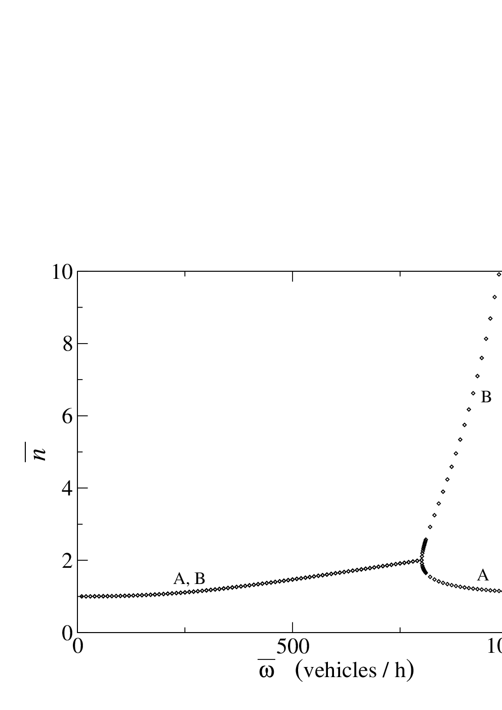
For this example we determined the solutions and with the control parameter varying from to about vehicles/hour. Figure 7 shows the results represented in the plane of coordinates . In the branch marked ‘A,B’ the parameter runs from zero in the upper lefthand corner to a critical value h-1 at a point where the curve bifurcates. The interpretation is that for the two lanes and have identical behavior; but when reaches its critical value, the symmetric solution becomes unstable and the symmetry between the lanes and is spontaneously broken. From the bifurcation point two branches marked A and B emanate; in the figure runs from to a value of the order of vehicles/hour along these branches. Lane has a high total density of vehicles, many of which are included in platoons, and the other lane has a lower density of vehicles, the majority of which are leading, and thus many of them must constitute 1-platoons. The continuation of the ‘A,B’ branch, where the symmetric solution is unstable, has been indicated as a dashed line.
Figure 8 shows, as a function of the control parameter , the densities and of the leading and following vehicles, as well as their sum . Figures 10 and 11 show the corresponding graphs of the average platoon length and the average platoon velocity . For small we are in the weakly interacting regime. The three densities shown in figure 8 are linear in , with deviations from linearity becoming appreciable when attains values of a few hundred vehicles/hour. We recall now that is also the density of platoons. Figure 8 shows that for small the platoon density is practically equal to the total vehicles density , which means that most vehicles constitute -platoons by themselves. This is confirmed by the initial behavior of in figure 10. Consistently, in figure 11 stays initially equal to its noninteracting value .
Beyond the small regime the average platoon velocity begins to decrease due to faster vehicles getting trapped in slow platoons. The instability occurs, in this example, when the average platoon length has increased to about two cars per platoon and the average platoon speed has gone down to about km/h. The interpretation of this symmetry breaking is most easily derived from the large behavior of the two branches. As increases to values well above , there occurs formation of a few very long platoons behind vehicles having velocities close to the minimum velocity. This explains why on branch asymptotically and . The small number of platoons in this lane have large spaces between them which allow the vehicles in lane to overtake almost without having to queue. Hence asymptotically on the branch . This interpretation is again confirmed by the figures 8, 10, and 11. Particularly striking is the rapid increase of the average platoon length in lane when increases in the supercritical regime. It returns to the average vehicle velocity in the absence of interaction; in lane it tends asymptotically to the velocity km h-1 of the slowest vehicles.
We note that the bifurcation points of and seem to coincide in figure 8, but figure 9 shows that they are actually distinct.
Finally in figure 12 we show the behavior of the effective velocity for two values of . They all have the expected behavior. For the subcritical flux vehicles/hour the functions and coincide. For the supercritical value vehicles/hour they are distinct; the lane curve is not far from the straight line valid for the noninteracting case, and in the lane curve the effective velocities are reduced to values not far from the minimum velocity km/h.
We have varied the distribution and found that this does not affect the qualitative features of the results that we discussed.




4.2 Symmetric lanes with PBC
It is worthwhile also to see what happens when the open boundary conditions (OBC) are replaced by periodic boundary conditions (PBC). For one thing, PBC may be easier in simulations of this and other models. In the case of PBC the density is given and the total vehicle density is the control parameter. We have studied the example where is the same truncated Gaussian, discretized on points , that was used in section 4.1.
The flux is now a derived quantity. We may decompose it as the sum of the fluxes and of leading and following vehicles, respectively. In figure 13 we have plotted and as functions of . Both bifurcate at a critical point km-1.
The behavior of the densities and may also be found as a function of ; it is very similar to the case of OBC, but with the difference that their sum is now a nonbifurcating straight line of unit slope. It thus appears that OBC and PBC lead to the same qualitative pictures. The qualitative features again remain unchanged as one varies the distribution .
4.3 Non-symmetric lanes with OBC
There are many ways to break the symmetry between the two lanes. We have chosen to investigate the open-ended problem with , all other things in the two lanes being identical. In particular, is again the Gaussian distribution of equations (4.1b)-(4.1c). We have taken a small symmetry breaking represented by and solved again equations (A.2) for and . Instead of figure 7 we now obtain figure 14, in which again the dashed lines represent (only schematically) branches of unstable solutions. Correspondingly, instead of the curves marked L, LA, and LB of figure 8 we now obtain the curves in figure 15. For low values of (and concomitantly ) the platoon densities in the two lanes (the curves marked LA and LB) increase linearly with , their slopes having a ratio 1 : 0.95. When increases, the critical point is avoided and the platoon density of lane (lane ) evolves continuously to the values represented by the branch marked LA1 (LB1). However, there is now a new critical value of 901 h-1 at which an inversion of the densities becomes possible. The two lanes are then on the ‘secondary’ branches LA2 and LB2.
We are in the presence of a stationary state problem for which there is no obvious way to define a free energy functional, although this may not be impossible. However, it seems reasonable to consider this set of secondary branches as ‘metastable’ (in the sense of having a higher free energy) with respect to the main branches.
4.4 Upper density limit
As we have seen in section 2.5, there is a high density regime where the present model ceases to be valid. The condition for validity depends on the external parameter , which represents the typical distance between two consecutive vehicles in a platoon. For the example of equations (4.1) we may estimate m, which when used in equation (2.56) gives
| (4.2) |
As we have seen, the principal phenomenon investigated in this work, namely the spontaneous symmetry breaking between two traffic lanes, occurs at a density of vehicles/km. Our conclusions concerning this phenomenon are therefore compatible with the simplifications of zero vehicle length and zero platoon length that we used.
5 Mathematical remarks
In this penultimate section we collect some comments on the calculations presented at various stages of this work with the purpose of clarifying their precise mathematical status.
The one-lane model is a statistical ensemble of geometrical constructs of the type represented in figure 6. This ensemble is defined by (i) the construction rules of sections 1 and 2; and (ii) as an input, the statistics of the intersections of the vehicle trajectories with one of the boundaries of the space-time domain, either the or the axis. One of the simplest ways of realizing (ii) would be to assume Poisson statistics for the intersection points and to assign to the vehicles velocities drawn independently from a given distribution, whether or . More generally, however, one could on the boundary specify arbitrary correlations between the positions and the velocities of the vehicles.
To develop the theory we have imposed, in addition to or , only the average flux or average density , but have not specified any boundary correlations. Our theory is therefore essentially a set of relations between average densities, fluxes, velocities, etc.
In section 2.1.3 the existence of a stationary state and a well-defined function is strictly speaking an assumption, however natural it may be. We leave open the possibility that the stationary state correlations (but not the averages) depend on the unspecified boundary correlations.
On only two occasions did the stationary state correlations between the vehicles play a role and was an extra assumption about them needed. The first occasion was when we discussed the statistics of platoon lengths in section 2.2.4; this calculation was accessory and had no bearing on the rest of the paper. The second occasion was in section 3.2 and appendix F, when we derived the function that connects the queuing times in one lane to the traffic density in the other one; although this connection is the very essence of the two-lane model, we expect that different assumptions about the correlations would lead to a qualitatively similar function . Nevertheless, in the single-lane model and for fully specified boundary statistics, it is a well-defined and still open question to determine the statistics of the platoon arrival times at a fixed observation point. We have not attempted in this work to answer that question and have simply presented the Poisson process nature of the arrival times as an additional hypothesis.
6 Summary and conclusion
In this paper we have proceeded in two steps.
First we defined a geometric traffic model of flux on a single lane (‘lane ’). The model includes the possibility for fast vehicles to overtake slower ones and is attractive because of its simplicity. Vehicle trajectories are straight lines except that overtaking vehicles incur time delays that follow from a given ‘queuing function’ , where is the velocity of the vehicle being overtaken. The single-lane model exhibits formation of platoons of vehicles. The platoon density as compared to the total vehicle density has been one of our main quantities of interest. We were able to relate analytically the platoon’s statistics to the flux intensity.
Secondly, and on the basis of additional hypotheses, we expressed the queuing function governing the lane vehicles in terms of the traffic conditions in the opposite lane, , and vice versa. This resulted in a set of coupled two-lane equations. Although the two lanes and have individually been modeled microscopically – that is, in terms of the trajectories of individual vehicles –, the two-lane equations connect densities and average velocities in the two lanes but no longer have a microscopic interpretation. We solved the two-lane equations numerically for a characteristic example of traffic flow with a priori identical traffic conditions on the two lanes (). It was found that above a critical traffic flux, , (or above a critical traffic density) the symmetry between the two lanes is spontaneously broken. One lane has fast traffic with mostly -platoons (= single vehicles), whereas the other lane has slow traffic with almost all vehicles queuing in long platoons. Asymmetric conditions have been briefly investigated, as well as the case where not the fluxes , but the spatial vehicle densities are the control parameters.
We argued that the model considered in this work is valid for low and moderate traffic densities. A more elaborate version, appropriately defined and including the parameter (= the typical intervehicle distance in a platoon), would be able to describe also the very high density regime and the phenomenon of jamming of one or both lanes. However, the spontaneous symmetry breaking reported in this paper occurs in the range of densities for which the present model is valid.
It has not been our purpose to be exhaustive. Several questions of interest have been left aside here but can be fairly straightforwardly treated in the same model. One of these concerns cases in which the velocity distribution has a tail that goes down to zero. Another one is the incorporation, along the road section under investigation, of entrance or exit ramps with prescribed vehicle fluxes. A less simple extension would be to include time-varying boundary conditions as may be due, for example, to traffic lights at the entrance of the road section. We have considered only the stationary state; studying the relaxation of an initial state towards stationarity would allow, among other things, a comparison with the scaling laws of reference [32].
Analytically various limit cases could be pursued further. In the weakly interacting limit an expansion of all relationships of this work in powers of and is certainly possible. In the limit where the variance of the velocity distribution becomes small, the phase transition point moves to higher densities; an expansion for small variance seems more complicated but nevertheless also possible. We have not exhibited any exact solutions to our equations; no doubt a few exist and we think some of these may be of interest.
The lane-lane coupling that we have introduced in the present study is of mean-field type, since each lane vehicle feels only the average effect of all lane vehicles, and vice versa. One should wonder if this approximation is justified and if in its absence the symmetry breaking still exists. We believe it does, the main argument being that each vehicle in one lane encounters in the course of time all vehicles in the other lane. This argument is admittedly heuristic. Some light is shed on its validity in two ways. First, in separate work [35] we found that the simulation of a closely related microscopic two-lane model also presents this symmetry breaking, at least on practically relevant scales of time and space. Secondly, in the quite different context of magnetic friction Hucht and coworkers [36, 37] were interested in an Ising system on a ladder lattice whose two legs are in relative motion. This model has essentially the same features as the present road traffic model; an exact solution [37] shows that there is a phase transition with mean-field characteristics for infinite relative velocity, which however gets rounded when the velocity becomes finite. We will leave further discussion of these issues to the future.
Appendix A Solution of Eq. 2.19 for
In this appendix we solve equation (2.19) for . We denote the numerator of its RHS by
| (A.1) |
This quantity satisfies
| (A.2) |
Upon setting we find that satisfies the linear equation
| (A.3) |
whence by differentiating twice we obtain
| (A.4) |
and
| (A.5) |
Setting now we can rewrite (A.5) as
| (A.6) |
Two successive integrations applied to (A.6) yield
| (A.7) |
and
| (A.8) |
where and are constants of integration. In order to determine these constants we first observe that (A.8) leads to . Since for the reasons exposed in section 1 we have , it follows that . Next we evaluate (A.4) for . Using that and this leads us to whence . Upon comparing this last result to (A.7) evaluated at we see that . Substitution of the values of and in (A.8) yields the solution (2.20) given in the main text. It is easily verified that for equation (2.20) reduces to , as had to be the case.
Appendix B An analytic example of functions and
B.1 Analytic example of
Let be a block distribution of the natural velocities,
let , and define the dimensionless parameter . Integrating according to equation (A.1) we first find
| (B.1) |
To abbreviate the notation we set
Next we find from equation (A.8) that
| (B.6) |
where is the indefinite integral
Depending on the values of the parameters and the variables of the problem, all three cases of this equation may occur. The desired function now follows by substitution of () in (B.6).
B.2 Limit of small
The above result becomes easier to visualize in the limit of small . In that limit the ‘arcoth’ applies in equation (). After a certain amount of algebra one obtains
| (B.12) |
in which the expression in brackets may be shown to be negative for all , as had to be the case because of . Expanding the coefficient of the term linear in near the lower limit of the velocity distribution we get
| (B.13) |
Let denote the effective velocity averaged with repect to at a given . Then we find from (B.1) together with (B.13)
| (B.14) |
in which is just the average natural velocity. In the limit of a narrow distribution, , this becomes
| (B.15) |
The factor shows that the reduction of the average effective velocity is proportional to the variance of the distribution.
B.3 Analytic example of
The platoon density corresponding to the present example is easiest to obtain from equation (2.35) [which is also (D.6)-(D.2)], from which has been eliminated. Upon observing that we get straightforwardly from (D.6) the simple expression
| (B.16) |
from which many further analytic results may be derived by means of the various relations of this work.
Appendix C Discretized equations
One may discretize the velocity axis by setting , where is a fixed increment. We let run from to some large value that may later on be set equal to infinity. The discretized version of the equations is used for the numerical solutions discussed in this work. It is, however, more than just a way of approximating the continuum limit, since it describes a traffic model having only a discrete set of velocities.
Open boundary conditions. Let us now take for the discrete distribution
| (C.1) |
and set
| (C.2) |
Upon substituting (C.1) and (C.2) in (2.19) and abbreviating we get for the equation
| (C.3) |
in which and where the right hand member depends only on . Given that we may obtain from this equation successively the numerical values of One can easily see that they are increasing with . Equation (C.3) is the discrete counterpart of (2.20). Its explicit solution is
| (C.4) |
with
| (C.5) |
When the velocities have the discrete distribution (C.1) we may set
| (C.6) |
and find that the discrete equivalent of (2.35) is
| (C.7) |
where we use the notation of appendix C.
Periodic boundary conditions. In the case of cyclic boundary conditions the density is the control function. Let us suppose it is of the discrete type
| (C.8) |
Substitution of this expression in (2.52) yields again expression (C.3) but with replaced with . Given that we may determine successively in the same way as for open boundary conditions.
Solving the equation explicitly yields
| (C.9) |
with
| (C.10) |
These two equations are the discrete versions of (2.51) and (2.47), respectively.
In the case of cyclic boundary conditions the expression for the density is again given by (2.27) but with replaced with . Its discrete equivalent, with an obvious definition of , is
| (C.11) |
Similarly, equation (2.32) has, in the case of cyclic boundary conditions, the discrete equivalent
| (C.12) |
When (C.9) is used in (C.12) we obtain after substantial rewriting the simplified result
| (C.13) |
with given by (C.10). Equations (C.13) and (C.10) constitute the discrete equivalent of (2.53) and (2.47) combined.
Appendix D Rewriting Eq. (2.32)
We consider here expression (2.32) for the platoon density ,
| (D.1) |
and show how it may be cast in a much simpler form. It is useful to abbreviate
| (D.2) |
Hence
| (D.3) |
and, for ,
| (D.4) |
Using (D.4) in (D.1) we obtain
| (D.5) | |||||
where to arrive at the second line we performed an integration by parts. When with the aid of (D.3) we eliminate the on the right hand side of (D.5) we obtain
| (D.6) | |||||
where we used that . Upon substituting for in the last line of (D.6) its definition (D.2) one obtains the final result of this rewriting, equation (2.35) of the main text.
Appendix E An equation for in the case of PBC
For the case of a single traffic lane with periodic boundary conditions, studied in section 2.3, we wish to find an expression for in terms of the control function . The reasoning resembles the one of subsection 2.2.2, but is still sufficiently different that we repeat the main steps here. Let be the time needed for a vehicle of natural velocity to cover a distance , that is, to complete one full turn of the ring. Then
| (E.1) |
We consider a marked vehicle of natural velocity and hence of effective velocity . Let and , so that . Let denote the average number of vehicles with velocities in the interval overtaken by the marked vehicle. To find an explicit expression for this number, we notice that the total number of vehicles on the ring having a velocity in the given interval is . Of these, the fraction overtaken by the marked vehicle is equal to times the relative distance covered, that is,
| (E.2) | |||||
As before, the time lost in overtaking a vehicle of velocity will be denoted by . Then, due to its overtaking of vehicles with velocities in , the marked vehicle, while it cycles the ring once, will be queuing during a total time that is given by
| (E.3) |
(in hybrid notation where we use both and variables). The total distance that it covers during this lost time is
| (E.4) |
Integrating now over all we find that the total time loss suffered by the marked vehicle during one cycle is
| (E.5) |
Similarly the total distance covered during this lost time is
| (E.6) |
In the remaining time interval the remaining distance is covered at a velocity . Hence we must have the key equation
| (E.7) |
We substitute (E.5) and (E.6) in this equation, using for the explicit expression (E.2). The result is the relation
| (E.8) |
When we divide by and transform from and to and using (2.9) we get
| (E.9) |
We can rewrite this as (2.45), which completes the proof and indirectly confirms the validity of (2.44) for the case of PBC.
Appendix F Relation between and
F.1 A problem in statistics
The question of finding a relation between and leads us to the following problem in statistics. Point events take place at a rate . We start observing them at an initial time . Let the stochastic variable denote the instant of time at which the first time interval starts that has a length greater than and is free of events. The probability distribution of will be of the form
| (F.1) |
where is the probability that there is no event in and where is the probability that the first eventless interval greater that starts in . The calculation of is possible but the expressions become more complicated than is needed for our purpose. We will therefore do something simpler, but good enough for our purpose, namely replace by its average
| (F.2) |
For dimensional reasons we can write
| (F.3) |
Furthermore we should necessarily have
| (F.4) |
It is not difficult to find an explicit expression for as defined by (F.2).
F.2 The expression for
Let be the probability that there is no event in , and let be the probability that the first time interval of length greater than comes along after the th event, for . Then
| (F.5) |
Using (F.2) we get
| (F.6) |
where is the average length of a time interval given that it is shorter than . An elementary calculation gives
| (F.7) | |||||
| (F.8) |
When (F.8) is substituted in (F.6) we get
| (F.9) | |||||
References
- [1] D. Chowdhury, L. Santen, and A. Schadschneider. Statistical Physics of Vehicular Traffic and some Related Systems. Phys. Rep., 329:199, 2000.
- [2] C. Appert and L. Santen. Boundary induced phase transitions in driven lattice gases with meta-stable states. Phys. Rev. Lett., 86:2498–2501, 2001.
- [3] R.J. Harris and R.B. Stinchcombe. Ideal and disordered two-lane traffic models. Physica A: Statistical Mechanics and its Applications, 354:582–596, 2005.
- [4] E. Pronina and A. B. Kolomeisky. Two channel totally asymmetric simple exclusion processes. J. Phys. A: Math. Gen., 37:9907, 2004.
- [5] Ekaterina Pronina and Anatoly B. Kolomeisky. Asymmetric coupling in two-channel simple exclusion processes. Physica A, 372:12–21, 2006.
- [6] Tobias Reichenbach, Erwin Frey, and Thomas Franosch. Exclusion processes with internal states. Phys. Rev. Lett., 97:050603, 2006.
- [7] Tobias Reichenbach, Erwin Frey, and Thomas Franosch. Traffic jams induced by rare switching events in two-lane transport. New J. Phys., 9:159, 2007.
- [8] Tobias Reichenbach, Thomas Franosch, and Erwin Frey. Domain wall delocalization, dynamics and fluctuations in an exclusion process with two internal states. The European Physical Journal E: Soft Matter and Biological Physics, 27:47–56, 2008.
- [9] C. Schiffmann, C. Appert-Rolland, and L. Santen. Shock dynamics of two-lane driven lattice gases. JSTAT, to appear, 2010.
- [10] H. van Beijeren. Private communication, 2010.
- [11] M. R. Evans, D. P. Foster, C. Godrèche, and D. Mukamel. Spontaneous symmetry breaking in a one dimensional driven diffusive system. Phys. Rev. Lett., 74:208, 1995.
- [12] C. Godreche, J.-M. Luck, M.R. Evans, D. Mukamel, and S. Sandow E.R. Speer. Spontaneous symmetry-breaking - exact results for a biased random-walk model of an exclusion process. J. Phys. A: Math. Gen., 28:6039–6071, 1995.
- [13] David W. Erickson, Gunnar Pruessner, B. Schmittmann, and R. K. P. Zia. Spurious phase in a model for traffic on a bridge. J. Phys. A: Math. Gen., 38:L659–L665, 2005.
- [14] R. D. Willmann, G. M. Schütz, and S. Grosskinsky. Dynamical origin of spontaneous symmetry breaking in a field-driven nonequilibrium system. Europhys. Lett., 71:542, 2005.
- [15] Stefan Großkinsky, Gunter M. Schütz, and Richard D. Willmann. Rigorous results on spontaneous symmetry breaking in a one-dimensional driven particle system. J. Stat. Phys., 128:587–606, 2007.
- [16] V. Popkov, M.R. Evans, and D. Mukamel. Spontaneous symmetry breaking in a bridge model fed by junctions. J. Phys. A: Math. Theo., 41:432002, 2008.
- [17] G. Korniss, B. Schmittmann, and R.K.P. Zia, Long-range order in a quasi one-dimensional non-equilibrium three-state lattice gas. Europhys. Lett., 45:431, 1999.
- [18] I. T. Georgiev, B. Schmittmann, and R. K. P. Zia. Anomalous nucleation far from equilibrium. Phys. Rev. Lett., 94:115701, 2005.
- [19] I. T. Georgiev, B. Schmittmann, and R. K. P. Zia. Cluster growth and dynamic scaling in a two-lane driven diffusive system. Journal of Physics A: Math. Gen., 39:3495–3509, 2006.
- [20] M. Ebbinghaus and L. Santen. A model for bidirectional traffic of cytoskeletal motors. J. Stat. Mech., page P03030, 2009.
- [21] S. Klumpp and R. Lipowsky. Phase transitions in systems with two species of molecular motors. Europhys. Lett., 66:90–96, 2004.
- [22] V. Popkov and G.M. Schütz. Shocks and excitation dynamics in a driven diffusive two-channel system. J. Stat. Phys., 112:523–540, 2003.
- [23] H.-W. Lee, V. Popkov, and D. Kim. Two-way traffic flow: exactly solvable model of traffic jam. J. Phys. A: Math. Gen., 30:8497, 1997.
- [24] Róbert Juhász. Dynamics at barriers in bidirectional two-lane exclusion processes. arXiv:0912.4608v1 (cond-mat.stat-mech), 2009.
- [25] M. Ebbinghaus, C. Appert-Rolland, and L. Santen. Bidirectional transport on dynamic networks. submitted to P.R.L. (arXiv:0912.3658), 2010.
- [26] V. Popkov and I. Peschel. Exactly solvable statistical model for two-way traffic. Journal of Physics A-Mathematical and General, 33:3989–3995, 2000.
- [27] V. Popkov and I. Peschel. Symmetry breaking and phase coexistence in a driven diffusive two-channel system. Phys. Rev. E, 64:026126, 2001.
- [28] Anna Melbinger, Tobias Reichenbach, Thomas Franosch, and Erwin Frey. Driven transport on parallel lanes with particle exclusion and obstruction. arXiv:1002.3766v1 [physics.bio-ph], 2010.
- [29] B. Schmittmann, J. Krometis, and R.K.P. Zia, Will jams get worse when slow cars move over? Europhys. Lett., 70:299 (2005).
- [30] E. Pronina and A. B. Kolomeisky. Spontaneous symmetry breaking in two-channel asymmetric exclusion processes with narrow entrances. J. Phys. A: Math. Gen., 40:2275–2286, 2007.
- [31] Rui Jiang, Ruili Wang, Mao-Bin Hu, Bin Jia, and Qing-Song Wu. Spontaneous symmetry breaking in a two-lane system with parallel update. J. Phys. A : Math. and Theo., 40:9213–9225, 2007.
- [32] E. Ben-Naim, P.L. Krapivsky, and S. Redner. Phys. Rev. E 50:822-829 (1994).
- [33] E. Ben-Naim and P.L. Krapivsky. Phys. Rev. E 56:6680-6686 (1997).
- [34] E. Ben-Naim and P.L. Krapivsky. J. Phys. A 31:8073-8080 (1998).
- [35] C. Appert-Rolland, H.J. Hilhorst, and G. Schehr (in preparation).
- [36] D. Kadau, A. Hucht, and D.E. Wolf. Magnetic Friction in Ising spin systems. Phys. Rev. Lett., 101:137205 (2008).
- [37] A. Hucht. Nonequilibrium phase transition in an exactly solvable driven Ising model with friction. Phys. Rev. E , 80:061138 (2009).