On well-separated sets and fast multipole methods
Abstract
The notion of well-separated sets is crucial in fast multipole methods as the main idea is to approximate the interaction between such sets via cluster expansions. We revisit the one-parameter multipole acceptance criterion in a general setting and derive a relative error estimate. This analysis benefits asymmetric versions of the method, where the division of the multipole boxes is more liberal than in conventional codes. Such variants offer a particularly elegant implementation with a balanced multipole tree, a feature which might be very favorable on modern computer architectures.
Keywords:
fast multipole method , balanced tree , asymmetric adaptive mesh , error analysis , Cartesian expansion.2010 MSC
65M15 , 65M80.1 Motivation
We consider in this paper a general error analysis and some implementation issues for fast multipole methods (FMMs). Since their first appearance in Greengard and Rokhlin [1987], Carrier et al. [1988], these tree-based algorithms have become important computational tools for evaluating pairwise interactions of the type
| (1.1) |
FMMs offer an -complexity and an a priori error estimate, but implementing a fully fledged adaptive FMM in 3D is a daunting task Cheng et al. [1999]. Parallelization issues complicate matter even further and call for a balance between, on the one hand theoretical efficiency, and on the other hand software complexity Shanker and Huang [2007], Vikram et al. [2009]. A major inconvenience with adaptive versions is the complicated memory access pattern which is due to the communication between levels in the multipole tree. Although this can be mitigated either through post-balancing algorithms Sundar et al. [2008], or by employing more advanced data-structures [Gumerov and Duraiswami, 2004, Chap. 6.6], with modern data-parallel architectures it has in fact been suggested that uniform versions offer better performance Gumerov and Duraiswami [2008].
An alternative is to use asymmetric adaptive meshes as outlined in Figures 1.1 and 4.1. Here the tree becomes balanced at the cost of a variable, but local, communication stencil. Also, the actual form of the multipole acceptance criterion becomes more critical as the mesh looses regularity. Comparisons between different criteria for cell-to-particle methods are found in Salmon and Warren [1994], while a careful worst-case analysis of uniform FMMs is found in Petersen et al. [1995].
The main contributions of the current paper are found in Sections 2 and 3 where the precise statement of the multipole acceptance criterion and the required assumptions on the kernel are discussed together with a general error analysis. Our approach is inspired by the treatment in the monograph Griebel et al. [2007], but we are able to offer several important corrections. In Sections 4 and 5 implementation issues are highlighted and we also perform numerical experiments illustrating the sharpness of the theory and the efficiency of the proposed approach.

2 Well-separated sets and kernel assumptions
We begin by stating the one-parameter criterion for two sets being well-separated. This is also a correction to the too weak criterion found in [Griebel et al., 2007, Eq. (8.31), p. 379].
Criterion 2.1 (-criterion).
Let the sets be contained inside two disjoint spheres such that and . Given , if , , and , then the two sets are well-separated whenever .
In other words, any of the two sets may be expanded by a factor of and arbitrarily rotated about its center point without touching the other set. When regarded as a parameter inside the FMM it will be evident that a smaller yields a smaller error at the cost of a larger communication stencil.
We remark that the -criterion under consideration is symmetric in its two arguments as a reflection upon the fact that we mainly consider FMMs where the sources and the evaluation points are “roughly” the same. — Indeed, our implementation as outlined in Section 4 produces a representation of the total field in the whole enclosing box under consideration. An algorithm which is adaptive in sources and evaluation points separately is described in [Gumerov and Duraiswami, 2004, Chap. 6.6; see also Fig. 5.1].
We shall need the following two simple consequences of the -criterion: since we get
| (2.1) | ||||
| Furthermore, writing the -criterion as , we also see that | ||||
| (2.2) | ||||
For and multi-indices in the normed space we write for brevity and additionally define factorials and powers in the usual intuitive manner. Similarly to [Griebel et al., 2007, Eq. (8.15), p. 317] (but here with an explicit factor ) we assume that the kernel ’s first few derivatives are equivalent to the harmonic potential:
Assumption 2.2 (Kernel regularity).
For with ,
| (2.3) | ||||
| where . Additionally, is positive and satisfies | ||||
| (2.4) | ||||
The analysis below takes place in -dimensional Cartesian space. In order to avoid the worst-case bound , assuming some kind of symmetry of the kernel seems inevitable (see also Shanker and Huang [2007]):
Assumption 2.3 (Rotational invariance).
For any rotation of the coordinate system,
| (2.5) |
In other words, we may freely rotate the coordinate system before expanding the kernel (provided of course that any expansion points are rotated as well). By choosing a such that , results obtained below in will be transferred to the Euclidean norm without introducing any constants.
3 Analysis
Consider now two points and , where and satisfy the -criterion. Approximating a unit source at using a far-to-far translation (, centered at ), followed by a far-to-local expansion (, centered at ), can be written as
| (3.1) |
with the order of the expansion. We consider the two errors in turn.
The integral form for the remainder of the -dimensional Taylor series becomes
using (2.3) and the multinomial theorem. As discussed in conjunction with Assumption 2.3 above we may now replace with . Using the triangle inequality and (2.2) yields so that from (2.4),
| (3.2) |
Using we readily bound the integrand and get
| (3.3) |
As for the first term in (3.1) we obtain this time a sum of integral remainders,
where the multinomial theorem and the rotational invariance were used twice. The sum can be evaluated when the upper limit tends to ; hence by uniform convergence,
Using (2.4), the triangle inequality, and (2.1) we get (compare with (3.2))
| (3.4) |
For the integrand we use the same type of bound as before and finally get
| (3.5) |
By summing the contributions (3.3) and (3.5) from positive potentials (cf. (2.4)) we thus conclude that the relative error for the th order fast multipole method under the -criterion is bounded by a .
In the above derivation we are lead to the -criterion by the initial requirement that . Clearly, the only natural way to obtain this is from the the triangle inequality and the slightly stronger requirement that (cf. (2.2)). Despite this clear reasoning we have not been able to find our version of the -criterion made explicit in the literature. Presumably, this is due to the fact that quadratic meshes are so popular.
We note also that the integral remainder term was consistently used instead of the Lagrangian version (hinted at also in Salmon and Warren [1994], Warren and Salmon [1995]). To see why, note that in bounding e.g. above we would otherwise obtain terms of the form with and . The only sensible bound now includes the factor suggesting that the convergence would deteriorate as . By contrast, the bounds (3.3) and (3.5) are perfectly regular for any .
It is to be stressed that we like to view the above analysis as a kind of template; the precise form of the assumptions and their implications are all very clearly visible. The effect of changing them can therefore readily be assessed.
4 Implementation
The current paper on the -criterion stems mainly from the fact that allowing an asymmetric adaptive splitting when creating the FMM mesh makes a convenient implementation possible. The ease of implementation is mainly thanks to the fact that the associated multipole tree is always balanced so that a static memory layout becomes natural. As a result, neighboring boxes are always arranged in the same level in the multipole tree, thereby facilitating the communication between them (see Figure 4.1 for an illustration).
We now give a brief description of our current implementation. For more detailed information the interested reader is kindly referred to the freely available code itself (see Section 5.1).
The multipole mesh is constructed first and is obtained by recursively splitting the source points at or near their median in each coordinate direction. A very fast and well-known algorithm is available for doing just this; this is the median-of-three selection algorithm which is most often used when implementing quicksort [Sedgewick, 1990, Chap. 9]. The source points themselves are naturally stored in a pyramid data-structure, a -tree cut at a certain maximum level [Gumerov and Duraiswami, 2004, Chap. 5.3].
After the sources have been assigned a box at the finest level, the connectivity information is determined. At any level in the tree the boxes are either decoupled or, respectively, strongly/weakly coupled. For each box , the strong connections of its parent box are examined; all children of a box in that satisfy the -criterion with respect to become weakly coupled to — the rest remain strongly coupled. This simple rule together with the fact that a box is always strongly connected to itself recursively defines the connectivity for the whole tree. The resulting topology is conveniently stored in sparse matrices with sparsity patterns known before each level is to be examined.
In the downward/upward phases the expansions are shifted as usual according to parent/child relations. The critical far-to-local shift follows the weak connectivity pattern and, at the finest level, the remaining strong connections are evaluated directly. As suggested in Deglaire et al. [2009], Coulaud et al. [2010] all shifts in the implementation tested below relies on BLAS Level 3 routines with constant transition matrices (using pre- and post-scaling according to the local geometry).
A few structural optimizations are optionally possible. For instance, a box weakly coupled to all children of a parent box can often interact via the latter instead (whenever the -criterion with respect to that parent is true). This is visible in Figure 1.1 where some of the weakly coupled grey boxes are noticeable large — here the interactions are in fact managed via parent boxes. A related idea at the finest level is to investigate strongly coupled boxes of very different radii, , say. If the -criterion is true when the roles of and are exchanged, then the sources in the larger box can be directly converted into a near field expansion in the smaller box, and the outgoing expansion from the smaller can simply be evaluated at each point in the larger box. This optimization was suggested already in Carrier et al. [1988].
Since it is beneficial to admit as large set of boxes as possible into the set of weak connections, it is natural to try to somehow locally relax the -criterion. Rather than uniformly enforcing a single value of for example, different ’s may well be accepted provided that an estimate of the total error remains bounded. For instance, if observed values of satisfy , then the relative error estimate is still . Ideas along these lines are discussed in Salmon and Warren [1994], Zhang and Tanaka [2007].


We conclude this section by very briefly discussing the algorithmic complexity. It is known that there typically exists extremely non-uniform distributions of source points that make most tree-codes (even the adaptive ones) run in time proportional to Aluru [1996]. Practical experience is usually much better, although for certain applications, simpler algorithms are occasionally preferred (see Blelloch and Narlikar [1997], and further the discussions in [Griebel et al., 2007, Chap. 8.7], and [Gumerov and Duraiswami, 2004, Chap. 6.6.3]).
In any case, the serial complexity for a 2D implementation using asymmetric adaptivity can be estimated to be roughly proportional to , since each of about boxes at the finest level is to interact through cluster-to-cluster interactions with on the order of boxes at the same level, and since each such shift requires on the order of operations. For a given relative tolerance , the analysis in Section 3 implies , so that the complexity is , thus indicating that the choice is nearly optimal. In practice, the best value of as well as the optimal number of subdivisions is rather dependent on the hardware and should be determined from experience. On balance we have found that the convenient choice and subdividing the points until the number of sources per box is works very well in practice.
5 Experiments
As illustrations to the analysis in Section 3 and in order to highlight some of the benefits with the proposed adaptivity we report some results from our two-dimensional implementation which employs the classical complex polynomial/multipole representation Greengard and Rokhlin [1987], Carrier et al. [1988].
Firstly, we investigated the sharpness of the -criterion and the accompanying error analysis. For this purpose, the complex-valued field was used and we calculated the total force in a system consisting of a million sources (see Figure 5.1 for results and further details of this simulation). Since is complex-valued the assumption (2.4) is clearly violated. Cancellation effects therefore implies that relative error estimates may well be impossible to obtain. Nevertheless, since the points are distributed randomly and an irregular mesh is used the effect is negligible in this case (although somewhat more prominent for the uniform distribution, see Figure 5.1).
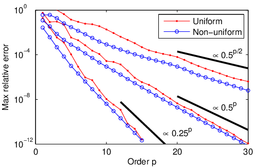
Secondly, we evaluated the efficiency of the proposed adaptivity at an effective relative tolerance of about (using expansion coefficients). Since our code is developed from a highly optimized uniform code outlined in Deglaire et al. [2009], a reasonably fair comparison is possible. Evidently, a square and uniformly subdivided multipole mesh implies a completely regular access pattern so that a highly efficient implementation using direct addressing techniques is possible. It is therefore of some interest to estimate under what circumstances adaptivity is actually beneficial. For this purpose we measured the speedup achieved by the adaptive code when the point sources were sampled from increasingly non-uniform data. The results are displayed in Figure 5.2 and shows that only for very uniform distributions of points is there a small gain () in using the uniform code.

As a third and final experiment we assessed the performance of the adaptive code for different point distributions. Using again a relative tolerance of , we measured the CPU-time for increasing number of points sampled from three very different distributions. As shown in Figure 5.3, the code is very robust indeed and scales well at least up to some 5 million point sources on a single CPU.

5.1 Reproducibility
Our two-dimensional implementation as described in Section 4 is available for download via the author’s web-page11 1 http://user.it.uu.se/~stefane/freeware. The code has been tested on several platforms, is fully documented, and comes with a convenient Matlab mex-interface. Along with the code, automatic Matlab-scripts that repeat the numerical experiments in Section 5 are also distributed. The results presented here were all obtained with a 3.06 GHz Intel Core 2 Duo processor with 4GB of internal memory running under Mac OS X 10.6.6.
6 Conclusions
Asymmetric adaptive meshes offer convenient and efficient FMM implementations. If cluster-to-cluster interactions are restricted to boxes for which the -criterion is true and if the kernel satisfies the assumptions outlined in Section 2, then the relative error can be bounded by a for and with the number of expansion terms. The computational complexity of the resulting 2D-algorithm can be expected to be about for some target tolerance . Not only is the actual performance of the algorithm competitive with optimized uniform FMMs even for relatively uniform data, but it is also robust for non-uniform distribution of points. Ongoing work includes porting the code to manycore platforms.
Acknowledgment
This work was supported by the Swedish Research Council within the FLOW and the UPMARC Linnaeus centers of Excellence.
References
- Aluru [1996] S. Aluru, Greengard’s -body algorithm is not order , SIAM J. Sci. Comput. 17 (1996) 773–776. doi:10.1137/S1064827593272031.
- Blelloch and Narlikar [1997] G. Blelloch, G. Narlikar, A practical comparison of -body algorithms, in: Parallel Algorithms, volume 30 of Series in Discrete Mathematics and Theoretical Computer Science.
- Carrier et al. [1988] J. Carrier, L. Greengard, V. Rokhlin, A fast adaptive multipole algorithm for particle simulations, SIAM J. Sci. Stat. Comput. 9 (1988) 669–686. doi:10.1137/0909044.
- Cheng et al. [1999] H. Cheng, L. Greengard, V. Rokhlin, A fast adaptive multipole algorithm in three dimensions, J. Comput. Phys. 155 (1999) 468–498. doi:10.1006/jcph.1999.6355.
- Coulaud et al. [2010] O. Coulaud, P. Fortin, J. Roman, High performance BLAS formulation of the adaptive fast multipole method, Math. Comput. Modelling 51 (2010) 177–188. doi:10.1016/j.mcm.2009.08.039.
- Deglaire et al. [2009] P. Deglaire, S. Engblom, O. Ågren, H. Bernhoff, Analytical solutions for a single blade in vertical axis turbine motion in two-dimensions, Eur. J. Mech. B Fluids 28 (2009) 506–520. doi:10.1016/j.euromechflu.2008.11.004.
- Greengard and Rokhlin [1987] L. Greengard, V. Rokhlin, A fast algorithm for particle simulations, J. Comput. Phys. 73 (1987) 325–348. doi:10.1016/0021-9991(87)90140-9.
- Griebel et al. [2007] M. Griebel, S. Knapek, G. Zumbusch, Numerical Simulation in Molecular Dynamics, volume 5 of Texts in Computational Science and Engineering, Springer Verlag, Berlin, 2007.
- Gumerov and Duraiswami [2004] N.A. Gumerov, R. Duraiswami, Fast multipole methods for the Helmholtz equation in three dimensions, Elsevier Series in Electromagnetism, Elsevier, Oxford, 2004.
- Gumerov and Duraiswami [2008] N.A. Gumerov, R. Duraiswami, Fast multipole methods on graphics processors, J. Comput. Phys. 227 (2008) 8290–8313. doi:10.1016/j.jcp.2008.05.023.
- Petersen et al. [1995] H.G. Petersen, E.R. Smith, D. Soelvason, Error estimates for the fast multipole method. II. The three-dimensional case, Proc. Math. Phys. Sci. 448 (1995) 401–418.
- Salmon and Warren [1994] J.K. Salmon, M.S. Warren, Skeletons from the treecode closet, J. Comput. Phys. 111 (1994) 136–155. doi:10.1006/jcph.1994.1050.
- Sedgewick [1990] R. Sedgewick, Algorithms in C, Addison-Wesley Series in Computer Science, Addison-Wesley, Reading, MA, 1990.
- Shanker and Huang [2007] B. Shanker, H. Huang, Accelerated Cartesian expansions - a fast method for computing of potentials of the form for all real , J. Comput. Phys. 226 (2007) 732–753. doi:10.1016/j.jcp.2007.04.033.
- Sundar et al. [2008] H. Sundar, R.S. Sampath, G. Biros, Bottom-up construction and 2:1 balance refinement of linear octrees in parallel, SIAM J. Sci. Comput. 30 (2008) 2675–2708. doi:10.1137/070681727.
- Vikram et al. [2009] M. Vikram, A. Baczewzki, B. Shanker, S. Aluru, Parallel accelerated Cartesian expansions for particle dynamics simulations, in: Proceedings of the 2009 IEEE International Parallel and Distributed Processing Symposium, pp. 1–11. doi:10.1109/IPDPS.2009.5161038.
- Warren and Salmon [1995] M.S. Warren, J.K. Salmon, A portable parallel particle program, Comput. Phys. Commun. 87 (1995) 266–290. doi:10.1016/0010-4655(94)00177-4.
- Zhang and Tanaka [2007] J.M. Zhang, M. Tanaka, Adaptive spatial decomposition in fast multipole method, J. Comput. Phys. 226 (2007) 17–28. doi:10.1016/j.jcp.2007.03.032.