Improved microscopic-macroscopic approach incorporating the effects of continuum states

The Woods-Saxon potential is a finite-depth potential, which has a continuum spectrum of unlocalized states as well as a discrete spectrum of localized states. Combined with a spin-orbit and proton’s Coulomb potentials, it resembles very well the potentials for a nucleon in atomic nuclei, having a flat central part and a short-range tail. The expression we employ is given by

$$H_{\rm WS}=\frac{\bm{p}^{2}}{2m}+V_{\rm CE}+V_{\rm SO}+\frac{1}{2}\left(1-\tau_{3}\right)V_{\rm CO},$$

(1)

where the central part $V_{\rm CE}$ and the spin-orbit part $V_{\rm SO}$ are the standard ones [43],

$$V_{\rm CE}=V_{\rm WS}(\bm{r};V_{\rm 0CE},\kappa_{\rm CE},R_{\rm 0CE},a_{\rm CE},\bm{\beta}),$$

(2)

$$V_{\rm SO}=\lambda_{\rm SO}\left(\frac{\hbar}{2m_{\rm red}c}\right)^{2}\Bigl(\bm{\nabla}V_{\rm WS}(\bm{r};V_{\rm 0CE},\kappa_{\rm SO},R_{\rm 0SO},a_{\rm SO},\bm{\beta})\Bigr)\cdot(\bm{\sigma}\times\frac{1}{i}\bm{\nabla}),$$

(3)

where $m_{\rm red}=\frac{A-1}{A}m$ with $m$ being the nucleon mass, $\tau_{3}$ the third component of the nucleon’s isospin multiplied by two (1 for neutrons and $-1$ for protons), $\bm{\sigma}$ the Pauli matrix for the nucleon’s spin ($\bm{s}=\frac{\hbar}{2}\bm{\sigma}$), and the function $V_{\rm WS}$ is defined by

$$V_{\rm WS}(\bm{r};V_{0},\kappa,R_{0},a,\bm{\beta})=-V_{0}\,\left[1\pm\kappa\frac{N-Z}{A}\right]\frac{1}{1+\exp[D(\bm{r};R_{0},\bm{\beta})/a]}.$$

(4)

Here, $N$, $Z$, and $A$ are the neutron, proton, and mass numbers, respectively, while $\pm$ in front of $\kappa$ means $+$ for proton and $-$ for neutron. $D(\bm{r};R_{0},\bm{\beta})$ denotes the (perpendicular) distance (with minus sign if $\bm{r}$ is inside the surface) between a given point $\bm{r}$ and the nuclear surface, so that $D(\bm{r};R_{0},\bm{\beta}=\bm{0})=r-R_{0}$ for spherical shape. The surface is specified by the radius $R_{0}$ and the deformation parameters $\bm{\beta}\equiv(\beta_{\lambda})$ as,

$$R(\theta;R_{0},\bm{\beta})=R_{0}\,c_{v}(\bm{\beta})\left[1+\sum_{\lambda}\beta_{\lambda}Y_{\lambda 0}(\theta)\right],$$

(5)

where the constant $c_{v}(\bm{\beta})$ takes care of the conservation of the volume inside the surface against deformation ($c_{v}=1$ for $\bm{\beta}=\bm{0}$). We consider only axially symmetric deformations and take into account the quadrupole ($\beta_{2}$) and hexadecapole ($\beta_{4}$) ones in this paper. The Coulomb potential $V_{\rm CO}$ acts only on protons, and is created by electric charge $(Z-1)e$ distributed uniformly inside the nuclear surface given by Eq. (5) with $R_{0}=R_{\rm 0CE}$.

The parameters $R_{\rm 0CE}$ ($R_{\rm 0SO}$) and $a_{\rm CE}$ ($a_{\rm SO}$) are the radius and the surface diffuseness of the central (spin-orbit) potential. For $N=Z$ nuclei, the depth of the central potential is $V_{\rm 0CE}$, while a dimensionless parameter $\lambda_{\rm SO}$ specifies the depth of the spin-orbit potential relative to the central potential. The quantities $\kappa_{\rm CE}$ and $\kappa_{\rm SO}$ describe the nuclear isospin dependence of the two potentials. Note that the radii and diffusenesses of the central and spin-orbit potentials are different in general, but the shape of nuclear surfaces are taken to be the same, i.e., the common deformation parameters $\bm{\beta}$ are used in both of them. The set of the values of these parameters mainly used to obtain the results shown in this paper is the universal parameter set of Ref. [43] (Note that the parameter $r_{0-\mbox{so}}(\mbox{P})=1.20$ in Table 1 of Ref. [43] is a misprint and should be replaced to $1.320$, see Ref. [44]). It should, however, be noted that we modify the depth of the central potential in order to be consistent with the liquid-drop Fermi energy; see Sec. III.8 for details.

The Nilsson potential is a harmonic oscillator potential combined with a spin-orbit and an $l^{2}$ terms. Since its depth (or height) is infinite, its spectrum does not have a continuum part. See, e.g., Ref. [45] for the equations to define the potential. We employ the $N_{\rm osc}$-dependent $ls$ and $l^{2}$ parameters of Ref. [46].

We use the anisotropic harmonic oscillator basis to diagonalize these single-particle Hamiltonians. The oscillator frequencies, $\omega_{3}$ and $\omega_{\bot}$, along the symmetry axis and the perpendicular axis, respectively, are determined by the two conditions; the volume conservation and the condition that they are inversely proportional to the root mean square length of each axis, which is calculated assuming the uniform sharp-cut density inside the nuclear surface given by Eq. (5). Namely the conditions are $\omega_{3}\omega_{\bot}^{2}=\omega_{0}^{3}$ and $\omega_{3}/\omega_{\bot}=\sqrt{\langle x^{2}\rangle_{\rm uni}/\langle z^{2}\rangle_{\rm uni}}\,$, where $\omega_{0}$ is the frequency for spherical shape and $\langle\;\rangle_{\rm uni}$ denotes average value based on the uniform sharp-cut density. The number of the basis states is specified by the total oscillator quantum number $N_{\rm osc}=n_{\bot}+n_{3}$ ($n_{\bot}=n_{1}+n_{2}$), where $n_{i}$ $(i=1,2,3)$ is the number of oscillator quanta in the $i$-th axis. In the following discussions, we use the standard harmonic oscillator energy, $\hbar\omega=41/A^{1/3}$ MeV, and the Woods-Saxon potential is diagonalized in the oscillator basis with a frequency $\omega_{0}=1.2\,\omega$.

In the shell correction method, the total energy of a nucleus is assumed to be decomposed as

$$E=E_{\rm mac}+\sum_{{\rm q}={\rm n},{\rm p}}\left(E_{\rm sh}^{(\rm q)}+E_{\rm pair}^{(\rm q)}\right),$$

(6)

where $E_{\rm mac}$ is the energy of a macroscopic model like the liquid-drop model while $E^{\rm(q)}_{\rm sh}$ and $E^{\rm(q)}_{\rm pair}$ are the microscopic corrections. Because the equations to define the contributions from neutrons (q=n) and protons (q=p) are very similar, we show only the terms for neutrons in the rest of this paper. For the sake of conciseness, we omit the superscript (n) for the most part, i.e., $E_{\rm sh}$ and $E_{\rm pair}$ designate $E_{\rm sh}^{(\rm n)}$ and $E_{\rm pair}^{(\rm n)}$, respectively.

The term $E_{\rm sh}$ is the shell correction energy, which is defined by

$$E_{\rm sh}=E_{\rm s.p.}-\tilde{E}_{\rm s.p.}.$$

(7)

The first term on the right-hand side is the sum of the single-particle energies of occupied levels,

$$E_{\rm s.p.}=\sum_{i=1}^{N}\epsilon_{i},$$

(8)

where $\epsilon_{1}\leq\epsilon_{2}\leq\cdots$ are the neutron single-particle energies. Since we are going to discuss about the Kruppa method (see Sec. II.4), these levels are the results of diagonalizations of the single-particle Hamiltonian in a truncated harmonic oscillator basis and thus they are discrete through negative and positive energies.

By introducing the (single-particle) level density,

$$g(\epsilon)=\sum_{i}\delta(\epsilon-\epsilon_{i}),$$

(9)

the quantity $E_{\rm s.p.}$ in Eq. (8) can be written as an integral,

$$E_{\rm s.p.}=\int_{-\infty}^{\lambda}\epsilon g(\epsilon)d\epsilon,$$

(10)

up to the Fermi energy $\lambda$. Analogously, the second term on the right-hand side of Eq. (7) is the integral of the product of the energy and a smoothed level density $\tilde{g}(\epsilon)$ over a semiinfinite energy interval up to the corresponding Fermi energenergy $\tilde{\lambda}$,

$$\tilde{E}_{\rm s.p.}=\int_{-\infty}^{\tilde{\lambda}}\epsilon\tilde{g}(\epsilon)d\epsilon,$$

(11)

with $\tilde{\lambda}$ determined to satisfy a constraint on the number of particles,

$$\int_{-\infty}^{\tilde{\lambda}}\tilde{g}(\epsilon)d\epsilon=N.$$

(12)

The term $E_{\rm pair}$ is the correction for the pairing energy, which is defined by

$$E_{\rm pair}=\left(E_{\rm BCS}-E_{\rm s.p.}\right)-\left(\tilde{E}_{\rm BCS}-\tilde{E}_{\rm s.p.}\right).$$

(13)

$E_{\rm BCS}$ and $\tilde{E}_{\rm BCS}$ are the energies of the BCS solutions of the pairing Hamiltonian with discrete and smoothed level densities, respectively. The terms in the first parentheses in the right-hand side represent the energy gain due to the pairing correlation. The terms in the second parentheses are the part of the pairing energy gain smoothly changing as a function of $N$ and $Z$, which should be subtracted since it is already included in $E_{\rm mac}$. Explicit expressions for these quantities are given in Secs. III.4 and III.6.

Using Eqs. (7) and (13), one can simplify Eq. (6) as

$$E=E_{\rm mac}+\sum_{\rm q=n,p}\left(E^{\rm(q)}_{\rm BCS}-\tilde{E}^{\rm(q)}_{\rm BCS}\right).$$

(14)

However, from a physical point of view, we discuss $E_{\rm sh}$ and $E_{\rm pair}$ separately. It may be worth noticing that one often uses simplified expressions for the smoothed part of the pairing energy in many of existing calculations, e.g., Refs. [10, 15], assuming that the single-particle levels are uniformly distributed with the smoothed level density at the Fermi energy. In such cases Eq. (14) does not hold exactly. In this paper we calculate $\tilde{E}_{\rm BCS}$ consistently without such simplifications, as is discussed in Secs. III.4 and III.6.

As for the energy of the macroscopic part, we use the liquid-drop model of Ref. [47] in this paper; see also Ref. [48] for its explicit form.

In the conventional Strutinsky smoothing method, the smoothed level density is obtained by a convolution integral with respect to the single-particle energy,

$$\tilde{g}(\epsilon)=\frac{1}{\gamma}\int_{-\infty}^{\infty}g(\epsilon^{\prime})f_{p}\left(\frac{\epsilon-\epsilon^{\prime}}{\gamma}\right)d\epsilon^{\prime},$$

(15)

where $f_{p}(x)$ is a smoothing function normalized as ${\displaystyle\int_{-\infty}^{\infty}f_{p}(x)dx=1}$, while $\gamma$ is the width parameter. The smoothing function is chosen as

$$f_{p}(x)=\frac{1}{\sqrt{\pi}}e^{-x^{2}}L^{1/2}_{p}(x^{2}).$$

(16)

Here, $L^{1/2}_{p}(x)$ is a polynomial of order $p$ (the generalized or associated Laguerre polynomial [49]), with which the transformation (15) leaves $g(\epsilon)$ unchanged, i.e., $\tilde{g}(\epsilon)=g(\epsilon)$, if $g(\epsilon)$ is a polynomial of order $2p$. Note that the order of polynomial is denoted by “$p$” in, e.g., Refs. [16, 26, 27], so that the parameter $p$ in these references is $2p$ in this work. Fig. 1 (a) shows the graphs of $f_{p}(x)$ for several values of $p$.

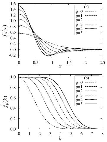
For a discrete level density,

$$g(\epsilon)=\sum_{i=1}^{M}\delta(\epsilon-\epsilon_{i}),$$

(17)

the smoothed density is given by

$$\tilde{g}(\epsilon)=\frac{1}{\gamma}\sum_{i=1}^{M}f_{p}\left(\frac{\epsilon-\epsilon_{i}}{\gamma}\right),$$

(18)

where $M$ is the number of single-particle levels included in the calculations. Owing to the gaussian form factor in $f_{p}(x)$, this transformation has a short-range character, which is a large advantage because it makes high positive energy levels unnecessary to evaluate Eq. (11) since they hardly affect $\tilde{g}(\epsilon)$ at negative energies.

Let us unveil another aspect of this transformation. The Fourier transform of a convolution of two functions is proportional to the product of each function’s Fourier transform. Therefore, by denoting the Fourier transform of a function $F$ as $\hat{F}$ like

$$\hat{F}(k)=\int_{-\infty}^{\infty}F(x)\,e^{-ikx}dx,$$

(19)

one can rewrite Eq. (15) as

$$\hat{\tilde{g}}(\tau)=\hat{f}_{p}(\gamma\tau)\,\hat{g}(\tau).$$

(20)

(A similar expression in terms of the Laplace transformation is given in Ref. [38] in a different context.) The “wavenumber” $\tau$ in Eq. (20) has a dimension of (energy)^-1 and may be regarded as a time variable (divided by $\hbar$). Now, we show that the function $\hat{f}_{p}$ has a typical shape of a low-pass filter. The Laguerre polynomial can be expressed in terms of the Hermite polynomials $H_{2l}$ as,

$$L^{1/2}_{p}(x^{2})=\sum_{l=0}^{p}C_{l}H_{2l}(x),\quad C_{l}=(-)^{l}(2^{2l}l!)^{-1}.$$

(21)

By multiplying $e^{-x^{2}}$ to the generating function of Hermite polynomials,

$$e^{-s^{2}+2xs}=\sum_{n=0}^{\infty}H_{n}(x)\,\frac{s^{n}}{n!},$$

(22)

one obtains

$$e^{-(s-x)^{2}}=\sum_{n=0}^{\infty}H_{n}(x)\,e^{-x^{2}}\,\frac{s^{n}}{n!}.$$

(23)

The Fourier transform of the left-hand side can be calculated easily as

$$\int_{-\infty}^{\infty}\,e^{-(s-x)^{2}}\,e^{-ikx}dx=\sqrt{\pi}\,e^{-k^{2}/4}e^{-iks}=\sum_{n=0}^{\infty}\sqrt{\pi}(-ik)^{n}e^{-k^{2}/4}\frac{s^{n}}{n!},$$

(24)

which means that the Fourier transform of $H_{n}(x)e^{-x^{2}}$ is

$$\int_{-\infty}^{\infty}\,H_{n}(x)e^{-x^{2}}dx=\sqrt{\pi}(-ik)^{n}e^{-k^{2}/4}.$$

(25)

Using above results, one obtains the Fourier transform of the Strutinsky smoothing function as

$$\hat{f}_{p}(k)=\sum_{l=0}^{p}C_{l}(-ik)^{2l}e^{-k^{2}/4}=\left[\sum_{l=0}^{p}\frac{1}{l!}\left(\frac{k}{2}\right)^{2l}\right]e^{-(k/2)^{2}}.$$

(26)

The term in the square brackets is the Taylor series of $e^{(k/2)^{2}}$ truncated at order $2p$. For $k\ll k_{p}^{\rm cut}\equiv 2\sqrt{p}$, the term is very close to $e^{(k/2)^{2}}$ and hence $\hat{f}_{p}\simeq 1$, i.e., the filter is almost perfectly transparent. From this fact, one may give an alternative definition of the polynomial part of the Strutinsky smoothing function: It is a polynomial which minimizes the distortion of this low-pass filter in such a way that $\hat{f}_{p}^{(l)}(0)=0$ for $1\leq l\leq 2p+1$. For $k\gg k_{p}^{\rm cut}$, the term in the square brackets is much smaller than $e^{(k/2)^{2}}$ and thus $\hat{f}_{p}\simeq 0$, i.e., the filter is almost completely opaque.

In Fig. 1 (b), the Fourier transform $\hat{f}_{p}(k)$ of the smoothing function is shown for several values of $p$. One sees that they are almost a constant function near $k=0$ and decrease monotonically to zero. They become a half of the maximum around $k\approx k_{p}^{\rm cut}=2\sqrt{p}$ (except $p$=0). The length of the interval where the function drops from 90% to 10% of the maximum ($\hat{f}_{p}(0)=1$) is $\sim 2.5$ and almost independent of $p$. One can verify these features in Table 1. In this way, the usage of higher order polynomials lengthens the width of the filter. At the same time, it shortens the width of the smoothing function in Fig. 1 (a) in a complementary manner.

Since the width of the filter of order $p$ is proportional to $\sqrt{p}$, it is convenient to use variables scaled with $\sqrt{p}$, $k^{\prime}=k/\sqrt{p}$. In Fig. 2 (b), we show $\hat{f}_{p}(k^{\prime}\sqrt{p}\,)$ versus $k^{\prime}$ for several values of $p$. As the order $p$ is increased, the cutoff becomes sharper while the position of the cutoff converges to $k^{\prime}=2$ independent of $p$; it approaches a step function $\theta\left(2-|k^{\prime}|\right)$ in the limit of $p\rightarrow\infty$. Corresponding changes in the function $f_{p}$ can be found by using a dimensionless variable $x^{\prime}=\sqrt{p}\,(\epsilon-\epsilon^{\prime})/\gamma$ and a rescaled smoothing function $f_{p}(x^{\prime}/\sqrt{p}\,)/\sqrt{p}$ to rewrite Eq. (15) as

$$\tilde{g}(\epsilon)=\int_{-\infty}^{\infty}g(\epsilon-\gamma x^{\prime}/\sqrt{p}\,)f_{p}(x^{\prime}/\sqrt{p}\,)\,dx^{\prime}/\sqrt{p}.$$

(27)

In Fig. 2 (a), $f_{p}(x^{\prime}/\sqrt{p}\,)/\sqrt{p}$ is shown as a function of $x^{\prime}$ for several values of $p$. Although the convergence is slow, for very large values of $p$, $f_{p}(x^{\prime}/\sqrt{p}\,)/\sqrt{p}\simeq(\sin 2x^{\prime})/\pi x^{\prime}$, which can be obtained as the inverse Fourier transform of $\theta\left(2-|k^{\prime}|\right)$. The curve for $p=50$ is quite close to this function in the interval shown in the figure. For larger $x^{\prime}$, however, the rescaled smoothing function decreases much faster than $x^{\prime-1}$ due to the Gaussian form factor.

Using the semiclassical periodic-orbit theory, the quantum mechanical level density (17) for a certain class of potentials can be represented by a sum of contributions from classical periodic (closed) orbits, the so-called trace formula [50, 51, 52]. It is discussed that the origin of the gross shell structure can be well understood in terms of a few important short periodic orbits; for example, a beating pattern of the level density in the spherical billiard [53], the shell structure in deformed nuclei [54], and the supershells in metal clusters [55]. The smooth part of the energy corresponds to the gross shell structure, to which only short periodic orbits contribute. The low-pass filter expression (20) demonstrates clearly that the conventional Strutinsky smoothing cuts off the contributions of long periodic orbits with period (divided by $\hbar$) $\tau=k/\gamma\gg\tau_{p}^{\rm cut}$ for the filter $\hat{f}_{p}(k)$, where the cutoff period is $\tau_{p}^{\rm cut}\equiv k_{p}^{\rm cut}/\gamma=2\sqrt{p}/\gamma$.

If one changes $\gamma$ as $\gamma\propto\sqrt{p}$ for different choices of the order $p$ in the smoothing function, the cutoff period $\tau_{p}^{\rm cut}$ is independent of $p$, while the cutoff becomes sharper for larger $p$ value as is clearly seen in Fig. 2 (b). In Sec. II.6 and Sec. III.3, we use this fact for discussions on the plateau condition, i.e., the stability of the smoothed energy with respect to the smoothing width $\gamma$ and the order $p$ specifying the curvature correction polynomials.

For finite-depth potentials like the Woods-Saxon one, positive energy levels appear as continuum states. They also affect the energy of bound nuclei through Eqs. (11) and (18). Their contribution becomes larger when $\tilde{\lambda}$ is closer to zero. If one obtains the positive energy spectrum by diagonalizing the Hamiltonian in a truncated oscillator basis, the positive energy spectrum is not continuous but discrete. Thus one can calculate the summation in Eq. (18) straightforwardly. However, the result depends strongly on the size of the basis $M$. In fact, the smoothed level density (18) diverges in the continuous limit and so does the smoothed energy (11); it is monotonically increasing or decreasing as increasing the size of the basis [17, 16]. A practical way to avoid this problem is to restrict the size of the basis; it is recommended in Ref. [17, 15] to take $N_{\rm osc}^{\rm max}\approx 12$ for the harmonic oscillator basis. However, in such small bases, negative energy levels may not be sufficiently accurate as we will see in the followings (see, e.g., Fig. 4).

A way to circumvent the diverging single-particle level density $g(\epsilon)$ due to the particle continuum is to replace it with the so-called continuum level density $g_{\rm c}(\epsilon)$. In the case of spherically symmetric potentials, it is written as [19, 20],

$$g(\epsilon)\quad\Rightarrow\quad g_{\rm c}(\epsilon)=\sum_{i:{\mbox{\scriptsize bound}}}\delta(\epsilon_{i}-\epsilon)+\frac{1}{\pi}\sum_{lj}(2j+1)\frac{d\delta_{lj}(\epsilon)}{d\epsilon},$$

(28)

where $\delta_{lj}(\epsilon)$ is the scattering phase shift. This expression was used for the calculation of shell correction energy and it was found that the contributions of the particle continuum (the second term on the right-hand side) through $\tilde{E}_{\rm s.p.}$ are never negligible even in stable nuclei for finite-depth potentials [18, 21].

One can roughly regard the continuum level density as the difference between the full and the free level densities [20]. Taking the energy derivative of the phase shift in Eq. (28) means calculating the level density from the number of states. The number of states is actually proportional to the phase of the radial oscillation of the wavefunction because an increase in the phase by $\pi$ corresponds to the addition of one radial node in the box boundary condition. The phase shift is the difference of the phases between full and free solutions. Therefore, the definition in terms of the phase shifts is actually equal to taking the limit of infinite volume of the difference between the full and free level densities in a finite volume cavity.

This can be shown more rigorously. The generalization of Eq. (28) for non-spherically symmetric potentials is given by [23, 22]

$$g_{\rm c}(\epsilon)=\frac{1}{2\pi i}\,{\hat{\rm tr}}_{\mbox{$\epsilon$}}\left[S^{\dagger}(\epsilon)\frac{dS(\epsilon)}{d\epsilon}\right],$$

(29)

where $S(\epsilon)$ is the on-shell S-matrix corresponding to the single-particle Hamiltonian $H$ with energy $\epsilon$, and ${\hat{\rm tr}}_{\mbox{$\epsilon$}}$ means the restricted trace operation with respect to the eigenstates with energy $\epsilon$. Note that Eq. (29) contains the contributions from the bound states because they appear as poles of the S-matrix. This quantity is related to the time-delay [56], and shown to be identical to the trace of the difference between the full and free single-particle Green’s functions [23]. In this way, the level density can be written as

$$g_{\rm c}(\epsilon)=\frac{1}{\pi}\mbox{Im}\left[{\rm tr}\,\frac{1}{H-\epsilon}-{\rm tr}\,\frac{1}{H_{0}-\epsilon}\right],$$

(30)

where $H_{0}$ is the free Hamiltonian (with the repulsive Coulomb potential for proton), and ${\rm tr}$ here is the full trace operation. This expression clearly tells that both full and free level densities are divergent for positive energies but their difference is finite. It is used for investigation of the level density in Ref. [24] by using the Green’s function technique [57].

Inspired by Eq. (30), Kruppa has introduced a prescription [22], which is suitable to treat the particle continuum by the diagonalization method with, e.g., the harmonic oscillator basis. He has demonstrated that results with his prescription have much weaker dependence on the size of the basis and converge for enough large basis. Let us call his prescription the Kruppa method. This method changes the definition of $g(\epsilon)$ as the difference of the single-particle level density between the full Hamiltonian (including the potential) and the free-particle Hamiltonian,

$$g(\epsilon)\quad\Rightarrow\quad g^{\rm K}(\epsilon)=\sum_{i=1}^{M}\delta\left(\epsilon-\epsilon_{i}\right)-\sum_{j=1}^{M}\delta(\epsilon-\epsilon^{0}_{j}),$$

(31)

where $\epsilon_{i}$ and $\epsilon^{0}_{j}$ are the eigenvalues of the full and the free Hamiltonians, respectively. Here $M$ is the dimension of the basis commonly used in the two diagonalizations, and $g^{\rm K}(\epsilon)\rightarrow g_{\rm c}(\epsilon)$ as $M\rightarrow\infty$ (see Eq. (30)). Note that, for one-body observables like the total single-particle energy in Eq. (10), the free energy terms in Eq. (31) do not contribute as long as $\lambda<0$, i.e., when the Fermi energy does not exceed the particle threshold. However, they contribute to the smoothed quantities. Now the smoothed level density $\tilde{g}(\epsilon)$ should be obtained by applying the Strutinsky smoothing to this $g^{\rm K}(\epsilon)$:

$$\tilde{g}(\epsilon)\quad\Rightarrow\quad\tilde{g}^{\rm K}(\epsilon)=\frac{1}{\gamma}\sum_{i=1}^{M}f_{p}\left(\frac{\epsilon-\epsilon_{i}}{\gamma}\right)-\frac{1}{\gamma}\sum_{j=1}^{M}f_{p}\left(\frac{\epsilon-\epsilon^{0}_{j}}{\gamma}\right).$$

(32)

The redefined level density $\tilde{g}^{\rm K}(\epsilon)$ converges to $\tilde{g}_{\rm c}(\epsilon)$ for sufficiently large basis sizes, the reason of which is explained transparently in Sec. II.5.

The continuum level density was originally used to calculate the second virial coefficient (related to the deviation of the equation of state from that for the ideal gas) arising from the interaction between gas particles [19, 20]. For this purpose, one naturally has to separate the part corresponding to the free motion of non-interacting particles from the integral over the continuous spectrum. Unlike this case, the reason to subtract the free spectrum is not so obvious in the calculation of the shell correction. At present, we do not know whether it can be derived rigorously from a more basic theoretical framework. Nevertheless, it certainly seems to be the most reasonable prescription so far to obtain physically meaningful results.

In Fig. 3 we show three kinds of level densities, i.e., the full (with Woods-Saxon potential), the free, and the Kruppa for ¹⁶⁴Er. They are the results of the Strutinsky smoothing with $\gamma=1.2\,\hbar\omega$ and $p=3$. The potential is deformed with $\beta_{2}=0.27$ and $\beta_{4}=0.02$. The number of basis states $M$ in Eq. (31) is specified by the maximum number of the oscillator quanta $N_{\rm osc}^{\rm max}$, $M=\frac{1}{3}(N_{\rm osc}^{\rm max}+1)(N_{\rm osc}^{\rm max}+2)(N_{\rm osc}^{\rm max}+3)$. Comparing panels (a), (b) and (c), one can see that positive energy part of the full and the free level densities are increased rapidly as $N_{\rm osc}^{\rm max}$ is increased from 12 to 20 and to 30, while the Kruppa’s level density does not change essentially. This clearly shows the fact that continuum parts of both the full and free densities are divergent but their difference is convergent. The energy range of the most influential part is $\epsilon\leq\lambda$ for the smoothed single-particle energy $\tilde{E}_{\rm s.p.}$ and $\left|\epsilon-\lambda\right|\leq\Lambda\sim\hbar\omega$ for the smoothed BCS energy $\tilde{E}_{\rm BCS}$. Though the difference in this part between the calculated level density with $N_{\rm osc}^{\rm max}=12$, 20 and 30 is much smaller than that in positive energy, e.g., at $\epsilon\sim 10$MeV, it brings about significant differences to the resulting nuclear properties, especially to the pairing correlation (see Sec. III.7).

All the smoothed quantities in the Kruppa method are obtained by replacing $\tilde{g}(\epsilon)$ with $\tilde{g}^{\rm K}(\epsilon)$. The shell correction energy $E_{\rm sh}$ by this prescription is investigated in Ref. [27], and shown to be also convergent when increasing the size of the basis. Examples are depicted in Fig. 4 as functions of the basis cutoff $N_{\rm osc}^{\rm max}$. Without the Kruppa’s prescription, $E_{\rm sh}$ depends on the size of the basis even in a stable nuclei ¹⁶⁶Er, and the dependence is much stronger in a neutron rich nuclei ²²⁶Er. The subtraction of the continuum contributions reduces the dependence on the model space drastically and the shell correction energy with the Kruppa method converges in the large $N_{\rm osc}^{\rm max}$ limit. These examples clearly show that the Kruppa’s prescription is indeed promising. We extend it for other observables in Sec. III.5.

It is also worth noting that while the shell correction energy $E_{\rm sh}$ almost converges at $N_{\rm osc}^{\rm max}\approx 12$, the sum of the single-particle energies $E_{\rm s.p.}$ itself does not; especially for the unstable nuclei ²²⁶Er the single-particle energies are not obtained very accurately when $N_{\rm osc}^{\rm max}\leq 20$. From this fact one may compose a syllogism on the necessity of the Kruppa method. (1) For large $N_{\rm osc}^{\rm max}$, the Kruppa method is necessary to treat correctly the dense positive energy spectrum. For small $N_{\rm osc}^{\rm max}$, it is not necessary. (2) One has to use large $N_{\rm osc}^{\rm max}$ for sufficiently accurate bound-state energies. (3) One needs the Kruppa method.

One can roughly reproduce the shape of the Kruppa’s level density in terms of a new variant of the Thomas-Fermi approximation within the limited phase space corresponding to the truncated oscillator basis. We call it the oscillator-basis Thomas-Fermi (OBTF) approximation in this paper. One can also demonstrate the independence of the results of the Kruppa method from $N_{\rm osc}^{\rm max}$ (if it is sufficiently large) in this approximation.

We study only spherically symmetric potentials without spin-orbit couplings. Lifting these restrictions is possible but does not seem to be very meaningful, because it turns out that the OBTF approximation is not sufficiently accurate to be used as a replacement of the smoothed energy in the realistic Strutinsky calculations. This corresponds to the known fact that, in order to obtain the Strutinsky smoothed energy, one has to include up to the third order terms in the semiclassical $\hbar^{2}$ expansion [38, 39], in which the Thomas-Fermi approximation is the lowest.

Hence we express the Hamiltonian for a nucleon as

$$H(p,r)=\frac{\bm{p}^{2}}{2m}+V(r),\;\;\;V(r)=V_{\rm CE}(r)+\frac{1}{2}\left(1-\tau_{3}\right)V_{\rm CO}(r),$$

(33)

where $V_{\rm CE}(r)$ and $V_{\rm CO}(r)$ are the central and Coulomb potentials in Sec.II.1 with spherical shape, i.e., with the deformation parameters $\bm{\beta}=\bm{0}$. The states are assumed to be doubly degenerated for the two spin states $s_{z}=\pm\frac{1}{2}$. In the Thomas-Fermi approximation, the number of particles in the potential well for a given single-particle energy $\epsilon$ is given by

$${\Gamma}(\epsilon)=4\pi\int_{0}^{\infty}\rho_{\!\!\phantom{.}{}_{\mbox{\tiny TF}}}(r,\epsilon)r^{2}dr$$

(34)

where $\rho_{\!\!\phantom{.}{}_{\mbox{\tiny TF}}}(r,\epsilon)$ is the particle density at position $r$ for Fermi level $\epsilon$ expressed as (using the Heaviside function $\theta$),

$$\rho_{\!\!\phantom{.}{}_{\mbox{\tiny TF}}}(r,\epsilon)=\frac{(2m)^{3/2}}{3\pi^{2}\hbar^{3}}\left|\epsilon-V(r)\right|^{3/2}\theta\left(\epsilon-V(r)\right).$$

(35)

The level density is related to the number of particles ${\Gamma}(\epsilon)$ as

$$g_{\!\!\phantom{.}{}_{\mbox{\tiny TF}}}(\epsilon)=\frac{d{\Gamma}(\epsilon)}{d\epsilon}=4\pi\int_{0}^{\infty}\frac{d\rho_{\!\!\phantom{.}{}_{\mbox{\tiny TF}}}(r,\epsilon)}{d\epsilon}r^{2}dr.$$

(36)

This level density diverges above the particle threshold, $\epsilon>0$, for finite-depth potentials because of the infinite volume of the space.

The idea of OBTF is to extend the Thomas-Fermi approximation in such a way that the phase space is limited within a subspace spanned by a truncated harmonic oscillator (HO) basis, which can be specified by the maximum kinetic energy as a function of position as in the followings. By replacing $V(r)$ with the oscillator potential $V_{\rm HO}(r)=\frac{1}{2}m\omega^{2}r^{2}$ in Eq. (35), one obtains

$${\Gamma}_{\rm HO}(\epsilon)=\frac{1}{3}\left(\frac{\epsilon}{\hbar\omega}\right)^{3},$$

(37)

which is always finite. A truncated oscillator basis is usually defined by the maximum oscillator quantum number $N_{\rm osc}^{\rm max}$. Equating the right-hand sides of Eqs. (37) to the number of states with $N_{\rm osc}\leq N_{\rm osc}^{\rm max}$ leads to the cutoff energy of the truncated basis, $\epsilon=\epsilon_{\rm cut}(N_{\rm osc}^{\rm max})$,

$$\epsilon_{\rm cut}=\hbar\omega\left[(N_{\rm osc}^{\rm max}+1)(N_{\rm osc}^{\rm max}+2)(N_{\rm osc}^{\rm max}+3)\right]^{1/3}.$$

(38)

We also define $R_{\rm max}$ by a condition $V_{\rm HO}(R_{\rm max})=\epsilon_{\rm cut}$, i.e.,

$$R_{\rm max}=\sqrt{\frac{2\epsilon_{\rm cut}}{m\omega^{2}}},$$

(39)

and the local maximum kinetic energy expressed as

	$\displaystyle\epsilon_{\rm kin}^{\rm max}(r)$	$\displaystyle=$	$\displaystyle\left(\epsilon_{\rm cut}-V_{\rm HO}(r)\right)\theta\left(\epsilon_{\rm cut}-V_{\rm HO}(r)\right)$		(40)
		$\displaystyle=$	$\displaystyle\frac{1}{2}m\omega^{2}\left(R_{\rm max}^{2}-r^{2}\right)\theta\left(R_{\rm max}-r\right).$

Now we define the level density in OBTF, similarly to Eq. (36), as

$$g_{\!\!\phantom{.}{}_{\mbox{\tiny OB}}}(\epsilon)=4\pi\int_{0}^{\infty}\frac{d\rho_{\!\!\phantom{.}{}_{\mbox{\tiny OB}}}(r,\epsilon)}{d\epsilon}r^{2}dr,$$

(41)

where $\rho_{\!\!\phantom{.}{}_{\mbox{\tiny OB}}}(r,\epsilon)$ is equal to the right-hand side of Eq. (35) with an additional restriction that the energy $\epsilon$ should be smaller than $\epsilon_{\rm kin}^{\rm max}(r)+V(r)$. Its derivative is given by (with the $\delta$-function contribution from the Heaviside function having no effects),

$$\frac{d\rho_{\!\!\phantom{.}{}_{\mbox{\tiny OB}}}(r,\epsilon)}{d\epsilon}=\frac{(2m)^{3/2}}{2\pi^{2}\hbar^{3}}\left|\epsilon-V(r)\right|^{1/2}\theta\left(\epsilon-V(r)\right)\theta\left(\epsilon_{\rm kin}^{\rm max}(r)+V(r)-\epsilon\right).$$

(42)

In this way, the finite level density $g_{\!\!\phantom{.}{}_{\mbox{\tiny OB}}}(\epsilon)$ is obtained for a given maximum oscillator quantum number $N_{\rm osc}^{\rm max}$.

The Kruppa’s level density $g_{\!\!\phantom{.}{}_{\mbox{\tiny OB}}}^{\rm K}(\epsilon)$ is defined as $g_{\!\!\phantom{.}{}_{\mbox{\tiny OB}}}^{\rm K}(\epsilon)=g_{\!\!\phantom{.}{}_{\mbox{\tiny OB}}}(\epsilon)-g_{\!\!\phantom{.}{}_{\mbox{\tiny OB}}}^{0}(\epsilon)$, where $g_{\!\!\phantom{.}{}_{\mbox{\tiny OB}}}^{0}(\epsilon)$ is the free-particle level density expressed as $g_{\!\!\phantom{.}{}_{\mbox{\tiny OB}}}^{0}(\epsilon)=4\pi{\displaystyle\int}\left[d\rho_{\!\!\phantom{.}{}_{\mbox{\tiny OB}}}^{0}(r,\epsilon)/d\epsilon\right]r^{2}dr$ with $\rho_{\!\!\phantom{.}{}_{\mbox{\tiny OB}}}^{0}(r,\epsilon)$ obtained by omitting $V(r)$ in the right-hand side of Eq. (42). (This is for neutrons and changes necessary for protons are described in the following paragraph). It is readily shown that

$$\Gamma_{\mbox{\tiny OB}}(\epsilon)=\int_{-\infty}^{\epsilon}g_{\!\!\phantom{.}{}_{\mbox{\tiny OB}}}(\epsilon^{\prime})d\epsilon^{\prime}=\frac{2(2m)^{3/2}}{\pi\hbar^{3}}\int_{\rm A}\epsilon_{\rm kin}^{1/2}\,r^{2}d\epsilon_{\rm kin}dr,$$

(43)

where $\epsilon_{\rm kin}=\epsilon^{\prime}-V(r)$, and the domain A of integration is depicted in panel (a) of Fig. 5. Changing the domain to B and C shown in panels (b) and (c) gives the similar expressions for ${\displaystyle\Gamma_{\mbox{\tiny OB}}^{0}(\epsilon)=\int_{-\infty}^{\epsilon}g_{\!\!\phantom{.}{}_{\mbox{\tiny OB}}}^{0}(\epsilon^{\prime})d\epsilon^{\prime}}$ and ${\displaystyle\Gamma_{\mbox{\tiny OB}}^{\rm K}(\epsilon)=\int_{-\infty}^{\epsilon}g_{\!\!\phantom{.}{}_{\mbox{\tiny OB}}}^{\rm K}(\epsilon^{\prime})d\epsilon^{\prime}}$, respectively. By enlarging the harmonic oscillator basis (i.e., by increasing $N_{\rm osc}^{\rm max}$ to ${N_{\rm osc}^{\rm max}}^{\prime}>N_{\rm osc}^{\rm max}$), domains A and B are expanded while domain C is left unchanged. The unchanged domain results in an unchanged number of levels and thus an unchanged level density. This explains pictorially why the Kruppa’s level density converges for large $N_{\rm osc}^{\rm max}$ above the particle threshold, $\epsilon>0$.

It is also possible to show that $g_{\!\!\phantom{.}{}_{\mbox{\tiny OB}}}^{\rm K}(\epsilon)\propto\epsilon^{-1/2}$ as $\epsilon\rightarrow\infty$ after the limit $N_{\rm osc}^{\rm max}\rightarrow\infty$ is taken. For an arbitrarily given $\epsilon>0$, one can take sufficiently large $N_{\rm osc}^{\rm max}$ to express the region C as $\left\{\left(\epsilon_{\rm kin},r\right)|\,0\leq r<\infty,\;\epsilon\leq\epsilon_{\rm kin}\leq\epsilon-V(r)\right\}$ with an approximation that $V(r)=0$ for $r>R_{\rm max}$ to obtain

$$\Gamma_{\mbox{\tiny OB}}^{\rm K}(\epsilon)\approx\frac{4(2m)^{3/2}}{3\pi\hbar^{3}}\int_{0}^{\infty}\left\{\left[\epsilon-V(r)\right]^{3/2}-\epsilon^{3/2}\right\}r^{2}dr.$$

(44)

Thus, for the level density $g_{\rm OB}^{\rm K}(\epsilon)=d\Gamma_{\mbox{\tiny OB}}^{\rm K}(\epsilon)/d\epsilon$,

	$\displaystyle\epsilon^{1/2}g_{\rm OB}^{\rm K}(\epsilon)$	$\displaystyle\approx$	$\displaystyle-\frac{2(2m)^{3/2}}{\pi\hbar^{3}}\int_{0}^{\infty}\frac{V(r)r^{2}dr}{1+\left[1-V(r)/\epsilon\right]^{1/2}}$		(45)
		$\displaystyle\rightarrow$	$\displaystyle-\frac{(2m)^{3/2}}{\pi\hbar^{3}}\int_{0}^{\infty}V(r)r^{2}dr\qquad(\epsilon\rightarrow\infty).$

It can be confirmed that the following expression is a very good approximation for the $N_{\rm osc}^{\rm max}\rightarrow\infty$ limit of the Kruppa level density in the whole range of single-particle energy:

$$g_{\!\!\phantom{.}{}_{\mbox{\tiny OB}}}^{\rm K}(\epsilon)\approx\frac{2(2m)^{3/2}}{\pi\hbar^{3}}\int_{0}^{\infty}\left[\left(\epsilon-V(r)\right)^{1/2}\theta\left(\epsilon-V(r)\right)-\epsilon^{1/2}\theta\left(\epsilon\right)\right]\,r^{2}dr.$$

(46)

For protons, one can repeat the same argument if one includes $V_{\rm CO}(r)$ in the free Hamiltonian, because $V_{\rm CO}(r)$ is not negligible even at $r=R_{\rm max}$ and $V(r)$ includes $V_{\rm CO}(r)$. In the same way, it is readily seen that the Kruppa level density is convergent as $N_{\rm osc}^{\rm max}\rightarrow\infty$ and in a very good approximation,

$$g_{\!\!\phantom{.}{}_{\mbox{\tiny OB}}}^{\rm K}(\epsilon)\approx\frac{2(2m)^{3/2}}{\pi\hbar^{3}}\int_{0}^{\infty}\left[\left(\epsilon-V(r)\right)^{1/2}\theta\left(\epsilon-V(r)\right)-\left(\epsilon-V_{\rm CO}(r)\right)^{1/2}\theta\left(\epsilon-V_{\rm CO}(r)\right)\right]\,r^{2}dr.$$

(47)

In Figs. 6 and 7, the OBTF level density is compared with the smoothed exact level density for a spherical nucleus ¹⁵⁴Er. Figure 7 includes the proton Kruppa densities. The spin-orbit force is neglected and a larger smoothing parameter $\gamma=1.8\hbar\omega$ is used with $p=3$ for this calculation to make the comparison more appropriate. One can see that the OBTF is a fairly good approximation for both $N_{\rm osc}^{\rm max}=12$ and $N_{\rm osc}^{\rm max}=20$. The proton Kruppa level density is very similar to the neutron one except that the single particle energy is shifted by the Coulomb barrier, about 10 MeV in this nucleus, as is shown in Fig. 7. Threshold behaviors of the OBTF neutron and proton level densities are slightly different, which reflects the effect of the long-range Coulomb potential, while such differences do not exist for the smoothed exact level densities.

Apart from oscillations at large $\epsilon$, the average behavior of the continuum level density is well reproduced in the OBTF approximation in Fig. 6. It can also be clearly seen how subtracting the free level density, Eq. (31), works to diminish the dependence on $N_{\rm osc}^{\rm max}$ in the Kruppa method. However, as it is clearly shown in Fig. 7, the precise shape of the smoothed level density cannot be obtained; especially, the peak near the threshold ($\epsilon\approx 0$) shows cusp behavior in the OBTF density, which is characteristic to the semiclassical approximation, while the smoothed density looks like a broad peak. In order to obtain more precise level density one has to go beyond the Thomas-Fermi approximation.

The Kruppa OBTF level density $g_{\!\!\phantom{.}{}_{\mbox{\tiny OB}}}^{\rm K}(\epsilon)$ becomes negative in the range of single-particle energy, $\epsilon_{\rm cut}+V(0)\leq\epsilon\leq\epsilon_{\rm cut}$ (see Fig. 6 (a)), and it can be shown, for a finite $N_{\rm osc}^{\rm max}$, that the positive and negative contributions exactly cancel out, ${\displaystyle\int_{-\infty}^{\infty}g_{\!\!\phantom{.}{}_{\mbox{\tiny OB}}}^{\rm K}(\epsilon)d\epsilon=0}$. This behavior is also known [24] in the exact continuum level density $g_{\rm c}(\epsilon)$ defined by Eqs. (28)$-$(30), and reflects the Levinson’s theorem [56], i.e., ${\displaystyle\int_{-\infty}^{\infty}g_{\rm c}(\epsilon)d\epsilon=0}$. In this way the OBTF Kruppa level density satisfies the desired property of the continuum level density.

It would be preferable if $\tilde{E}_{\rm s.p.}$ of Eq. (11) did not depend on the parameters concerning the smoothing of the level density ($\gamma$ and $p$ in Eq. (15)) because their values can be chosen arbitrarily. Since a perfect independence is unlikely to be satisfied, one usually demands a weaker condition that the dependence is very weak in a certain interval of $\gamma$ for a few values of $p$. This is the meaning of the plateau condition in this paper.

For the Nilsson spectrum, a long plateau appears in most cases (see, e.g., Ref. [9, 21]). On the other hand, for finite-depth potentials like the Woods-Saxon potential, the situation is subtle. If the oscillator basis is truncated at $N_{\rm osc}^{\rm max}\approx 10$ to $12$, reasonable plateau are obtained in many cases [17], and $N_{\rm osc}^{\rm max}=12$ is a recommend value as a working prescription in Ref. [15]. However, the model space defined by $N_{\rm osc}^{\rm max}=12$ is not large enough to calculate single-particle states accurately, especially for unstable nuclei (see, e.g., Fig. 4 (d)), and this truncation is not justified. The appearance of plateau obtained by the relatively small model space with $N_{\rm osc}^{\rm max}\approx 10$ to $12$ is accidental and increasing $N_{\rm osc}^{\rm max}$ drastically change the situation [17, 16]; the shell correction energy depends strongly on the smoothing width $\gamma$. This clearly indicates that a naïve inclusion of continuum states by the diagonalization method does not work. Then, the continuum level density, Eq. (28), is used to calculate the shell correction energy [18, 21]. Although the dependence on $\gamma$ is weaker if the phase shift is calculated up to enough high energies, no good plateau like in the case of the Nilsson potential is obtained [26].

We show examples in Figs. 8 to 11. Figures 8 and 9 depict the neutron shell correction energies $E_{\rm sh}$ calculated with the standard Strutinsky smoothing method and with the Kruppa-method, respectively, changing the basis size specified by the maximum oscillator quantum number $N_{\rm osc}^{\rm max}$. The results for the stable and unstable nuclei, ${}^{166}{\rm Er}$ and ${}^{226}{\rm Er}$, are compared. If $N_{\rm osc}^{\rm max}=12$ is used for the basis size, a plateau-like behavior is observed in a reasonably long range for ${}^{166}{\rm Er}$ and in a shorter range for ${}^{226}{\rm Er}$. But this is “spurious” because, using larger $N_{\rm osc}^{\rm max}$, the shell correction energy depends more strongly both on the smoothing width $\gamma$ and the order $p$ of the curvature correction polynomial, while the range of “real” plateau in the case of the harmonic oscillator potential grows as the basis size increases [25]. The possible reason of this “spurious” plateau is that the number of discretized continuum states with $N_{\rm osc}^{\rm max}=12$ is just suitable for the smoothed level density to be approximated by the lower order polynomial functions across the particle threshold $\epsilon\approx 0$. Increasing the basis size the curvature of the smoothed level density changes suddenly at $\epsilon\approx 0$, as is shown in Fig. 3, which no longer be approximated by a simple polynomial; leading to the strong dependence of $E_{\rm sh}$ on $\gamma$ and $p$. Therefore, it is difficult to obtain reliable shell correction energies in the standard Strutinsky method.

In contrast, the Kruppa’s prescription reduces the basis-size dependence dramatically, as can be seen in Fig. 9. Compared with the standard method, where the plateau condition is more and more unsatisfied as increasing the basis size, the stability against the increase of $N_{\rm osc}^{\rm max}$ is a very important feature of the Kruppa method. However, although there are almost degenerate local minima with different order $p$’s, the plateau is not well established generally. The situation is worse for unstable nucleus ²²⁶Er. A possible improvement will be discussed in Secs. III.1 to III.3.

At first sight, the dependence of the shell correction energy on the smoothing width $\gamma$ is quite different when the order $p$ of the smoothing function (16) is changed. Close inspection reveals, however, that the different curves in each panel of Figs. 8 and 9 are almost isomorphic if they are drawn as functions of the $\sqrt{p}\,$–scaled width parameter,

$$\gamma_{p}\equiv\gamma/\sqrt{p/3},$$

(48)

as shown in Figs. 10 and 11. Here we choose $\gamma_{p=3}=\gamma$ because $p=3$ is a standard choice for the curvature correction polynomial. The reason of this “isomorphism” between the results with different order $p$’s can be understood from the discussion in Sec.II.3; the range of the low-pass filter increases when employing the larger order $p$, and if is used the variable scaled with $\sqrt{p}$ the cutoff ranges are the same but the filter becomes sharper, as is clearly shown in Fig. 2 (b). Therefore, the complete isomorphism means the shell correction energy is independent of the sharpness of the filter. We have found that, for calculation with larger $N_{\rm osc}^{\rm max}$, better isomorphism is generally obtained by the Kruppa smoothing method than by the standard one; compare Fig. 10 with Figs. 11. Even better isomorphism is obtained in the improved treatment in Sec. III.1 (see Fig. 19). In the following discussions for the plateau condition, we always use the Kruppa prescription and show the results as functions of the $\sqrt{p}\,$–scaled width parameter $\gamma_{p}$ (48).

In the course of writing the present paper, we noticed that a similar scaled smoothing width is used for investigating the plateau condition in Ref. [58], where the isomorphism of the smoothing width dependence between different order $p$’s is not as good as in our case. This is due to a different choice of basic smoothing function that is not gaussian. We believe that the Fourier transform of the smoothing function will be useful for more detailed comparison of our results with those of Ref. [58].

A clue to find the origin of this difference between the Nilsson (or the harmonic oscillator) potential and the Woods-Saxon (or the finite-depth, in general) potential is the fact that the Strutinsky smoothing is a low-pass filter as discussed in Sec. II.3. In the Fourier transformed world, the smoothed level density is simply the original density multiplied by the filter. Therefore, the Fourier transform of the original level density (17), or the Kruppa density (31),

$$\hat{g}(\tau)=\sum_{i=1}^{M}\exp(-i\tau\epsilon_{i}),\qquad\hat{g}^{\rm K}(\tau)=\sum_{i=1}^{M}\exp(-i\tau\epsilon_{i})-\sum_{j=1}^{M}\exp(-i\tau\epsilon^{0}_{j})$$

(49)

should be investigated.

In this subsection, we employ the units $\hbar\omega$ for the energy ($\epsilon$, $\gamma$, and $\sigma$) and $(\hbar\omega)^{-1}$ for the Fourier transformed time variable $\tau$, and regard $\epsilon$ and $\tau$ as if they were dimensionless.

The level density $g(\epsilon)$ and its Fourier transform $\hat{g}(\tau)$ for the Nilsson potential are shown in Fig. 12 for the spherical nucleus ²⁰⁸Pb. The single-particle states up to $N_{\rm osc}^{\rm max}=9$ are included because the $ls$ and $l^{2}$ parameters are given only for them [46]. Fig. 12 (a) shows that the smoothed level density with $\gamma=1.2\,\hbar\omega$ is approximately a quadratic function in $\epsilon$, while the major shell oscillation is clearly seen in that with $\gamma=0.5\,\hbar\omega$. This indicates that the semiclassical property of the Nilsson spectra is essentially the same as that of the HO potential; its Thomas-Fermi level density is $g_{\!\!\phantom{.}{}_{\mbox{\tiny TF}}}^{\rm HO}(\epsilon)=\epsilon^{2}/(\hbar\omega)^{3}$, see Eq. (37). Note that the so-called “iso-stretching” is done for the neutron and proton frequencies in the Nilsson potential [45], $\omega_{\rm n}=(2N/A)^{1/3}\omega$ and $\omega_{\rm p}=(2Z/A)^{1/3}\omega$, so that the coefficient of $\epsilon^{2}$ is reduced by a factor $208/(2\times 126)$ in Fig. 12 (a).

Concerning the behavior of $\hat{g}(\tau)$ shown in Fig. 12 (b), one can see a very low density interval ($2<\tau<5$). One may probably call its origin as the harmonicity of the potential. If the cutoff period $\tau_{p}^{\rm cut}=2\sqrt{p}\gamma^{-1}$ of the filter $\hat{f}_{p}(\tau\gamma)$ is in this interval, the result of the filtering, $\hat{\tilde{g}}(\tau)$, hardly depends on $\tau_{p}^{\rm cut}$ (see Sec. II.3). Namely, the dependences on $\gamma$ and $p$ are weak and there appears a plateau. This feature can be qualitatively understood by considering the case of the anisotropic harmonic oscillator potential, for which the spectra are equidistant and the sum in Eq. (49) with $M\rightarrow\infty$ can be evaluated as an infinite geometric series to be

$$\hat{g}_{\rm HO}(\tau)=\left[(2i)^{3}\sin\left(\frac{1}{2}\tau\hbar\omega_{x}\right)\sin\left(\frac{1}{2}\tau\hbar\omega_{y}\right)\sin\left(\frac{1}{2}\tau\hbar\omega_{z}\right)\right]^{-1},$$

(50)

with $\omega_{x}\approx\omega_{y}\approx\omega_{z}\approx\omega$, which has a long low density interval between $\tau=0$ and $\tau=2\pi$ (in units of $(\hbar\omega)^{-1}$).

In contrast to the case of Nilsson potential, the Fourier transform of the Woods-Saxon level density shown in Fig. 13 does not have this low-amplitude region, although the smoothed level density in the panels (a) and (b) clearly shows the similar major shell oscillation to that in Fig. 12 (a). In Fig. 13 the Fourier transforms of not only the Woods-Saxon spectra but of the Kruppa spectra and of the restricted spectra within the bound states are also depicted. The Fourier transform of the bound-states spectra is smaller than that of the Woods-Saxon spectra, but is still about a factor two to three larger than that of the Nilsson spectra in the low density interval ($2<\tau<5$) (note the difference of scale in ordinates in Fig. 12 and 13). Moreover, the Fourier transform of the Kruppa spectra is larger than that of the Woods-Saxon spectra on average, and increasing the basis size makes the situation worse. This clearly shows that the Kruppa prescription does not help to make a plateau in the shell correction energy, which is already confirmed in the previous subsection. The mechanism to develop a long plateau in the Nilsson spectrum is not functioning in the Woods-Saxon spectrum. This seems to be the very reason for the absence of plateau for the Woods-Saxon spectrum.

The Woods-Saxon potential is different from the Nilsson potential not only in the anharmonicity but also in the finite depth. It seems interesting to investigate further the difference between negative and positive parts of the spectrum. In order to examine this point, the short-time Fourier transform [59] seems useful. It is defined by

$$\begin{array}[]{lll}\hat{F}(k,x;\sigma)&=&{\displaystyle\int_{-\infty}^{\infty}F(x^{\prime})w_{\sigma}(x^{\prime}-x)e^{-ikx^{\prime}}dx^{\prime},}\\ &=&{\displaystyle\frac{1}{2\pi}e^{-ikx}\int_{-\infty}^{\infty}\hat{F}(k^{\prime})\hat{w}_{\sigma}(k-k^{\prime})e^{ik^{\prime}x}dk^{\prime},}\end{array}$$

(51)

where for the window function $w_{\sigma}(\xi)$ and its Fourier transform we employ

$$w_{\sigma}(\xi)=e^{-(\xi/\sigma)^{2}},\qquad\hat{w}_{\sigma}(\kappa)=\sqrt{\pi}{\sigma}\,e^{-(\sigma\kappa/2)^{2}}.$$

(52)

In this paper we apply it to a “short energy interval” Fourier transform. Figures 14 to 16 show $\hat{g}(\tau,\epsilon;\sigma)$ with $\sigma=\sqrt{2}$, which gives the same size of window widths in two complementary variables $\tau$ and $\epsilon$. The same nucleus ²⁰⁸Pb is used for this calculation. The input level density $\tilde{g}(\epsilon)$ has been smoothed with $\gamma=1.2$ and $p=3$ in the right-hand panels (no smoothing has been done for the left-hand panels). The location of cutoff due to these smoothings are $\tau_{p}^{\rm cut}=2\sqrt{p}\gamma^{-1}=2.9$ for $\gamma=1.2$, but then the cutoff result is blurred by the convolution with the window function of width $\sqrt{2}/\sigma=1$ (see Eq. (51)).

References

- [1] J. Dobaczewski and W. Nazarewicz, Phill. Trans. R. Soc. Lond. A 356, 2007 (1998).
- [2] M. Arnould, S. Goriely, and K. Takahashi, Phys. Rep. 450, 97 (2007).
- [3] J. Dobaczewski, N. Michel, W. Nazarewicz, and M. Plaszajczak, Prog. Part. Nucl. Phys. 59, 432 (2007).
- [4] P. Ring and P. Schuck, The nuclear many-body problem, Springer, New York (1980).
- [5] M. Bender, P. -H. Heenen and P. -G. Reinhard, Rev. Mod. Phys. 75, 121 (2003).
- [6] D. Lunney, J. M. Pearson and C. Thibault, Rev. Mod. Phys. 75, 1021 (2003).
- [7] M. Strutinsky, Sov. J. Nucl. Phys. 3 449 (1966); Nucl. Phys. A95, 420 (1967).
- [8] M. Strutinsky, Nucl. Phys. A122, 1 (1968).
- [9] S. G. Nilsson, C. F. Tsang, A. Sobiczewski, Z.Szymanski, S.Wycech, C. Gustafsson, I. L. Lamm, P. Moller, and B. Nilsson, Nucl. Phys. A131, 1 (1969).
- [10] M. Brack, J. Damgård, A. S. Jensen, H. C. Pauli, V. M. Strutinsky, and C. Y. Wong, Rev. Mod. Phys. 44, 320 (1972).
- [11] M. Strutinsky, Nucl. Phys. A218, 169 (1974).
- [12] M. Brack and P. Quentin, Nucl. Phys. A361, 35 (1981).
- [13] S. Goriely, N. Chamel, and J. M. Pearson, Phys. Rev. Lett. 102, 152503 (2009).
- [14] S. Goriely, S. Hilaire, M. Girod, and S. Péru, Phys. Rev. Lett. 102, 242501 (2009).
- [15] P. Möller, J. R. Nix, W. D. Myers, and W. J. Swiatecki, At. Data Nucl. Data Tables 59, 185 (1995).
- [16] W. Nazarewicz, T. R. Werner, J. Dobaczewski, Phys. Rev. C 50, 2860, (1994).
- [17] M. Bolsterli, E. O. Fiset, J. R. Nix, and J. L. Norton, Phys. Rev. C 5, 1050 (1972).
- [18] Wing-fai Lin, Phys. Rev. C 2, 871 (1970).
- [19] E. Beth and G. E. Uhlenbeck, Physica 4, 915 (1937).
- [20] L. D. Landau and E. M. Lifshitz, Statistical Physics, §77, Pergamon (1958).
- [21] C. K. Ross and R. K. Bhaduri, Nucl. Phys. A188, 566 (1972).
- [22] A. T. Kruppa, Phys. Lett. B431, 237 (1998).
- [23] T. Y. Tsang and T. A. Osborn, Nucl. Phys. A247, 566 (1975).
- [24] S. Shlomo, Nucl. Phys. A539, 17 (1992).
- [25] M. Brack and H. C. Pauli, Nucl. Phys. A207, 401 (1973).
- [26] T. Vertse, A. T. Kruppa, R. J. Liotta, W. Nazarewicz, N. Sandulescu, and T. R. Werner, Phys. Rev. C 57, 3089 (1998).
- [27] T. Vertse, A. T. Kruppa, W. Nazarewicz, Phys. Rev. C 61, 064317 (2000).
- [28] G. G. Bunatian, V. M. Kolomietz, and V. V. Strutinsky, Nucl. Phys. A188, 225 (1972).
- [29] V. V. Strutinsky and F. A. Ivanjuk, Nucl. Phys. A255, 405 (1975).
- [30] F. A. Ivanyuk and V. M. Strutinsky, Z. Phys. A286, 291 (1978).
- [31] F. A. Ivanyuk and V. M. Strutinsky, Z. Phys. A290, 107 (1979).
- [32] F. A. Ivanyuk, Z. Phys. A316, 233 (1984).
- [33] F. A. Ivanjuk and V. V. Strutinsky, Z. Phys. A293, 337 (1979).
- [34] F. Tondeur, Nucl. Phys. A383, 32 (1982).
- [35] K. Pomorski, Phys. Rev. C 70, 044306 (2004).
- [36] R. K. Bhaduri and C. K. Ross, Phys. Rev. Lett. 27, 606 (1971).
- [37] M. Brack and R. K. Bhaduri, Semiclassical Physics (Addison-Wesley, Reading, MA, 1997).
- [38] B. K. Jennings, Nucl. Phys. A207, 538 (1973).
- [39] B. K. Jennings, R. K. Bhaduri, and M. Brack, Nucl. Phys. A253, 29 (1975).
- [40] A. Bhagwat, X. Vias, M. Centelles, P. Schuck, and R. Wyss, Microscopic-Macroscopic Approach for Binding Energies with Wigner-Kirkwood Method, preprint arXiv:0911.4648v1.
- [41] J. Dobaczewski, H. Flocard, and J. Treiner, Nucl. Phys. A422, 103 (1984).
- [42] W. D. Myers, Nucl. Phys. A145, 387 (1970).
- [43] S. Cwiok, J. Dudek, W. Nazarewicz, J. Skalski and T. Werner, Comp. Phys. Comm. 46, 379 (1987).
- [44] J. Dudek, Z. Szymanski and T. Werner, Phys. Rev. C 23, 920 (1981).
- [45] S. G. Nilsson and I. Ragnarsson, Shapes and Shells in Nuclear Structure, Cambridge University Press (1995).
- [46] T. Bengtsson and I. Ragnarsson, Nucl. Phys. A436, 14 (1985).
- [47] W. D. Myers and W. J. Swiatecki, Nucl. Phys. 81 1 (1966); Ark. Phys. 36, 343 (1967).
- [48] A. V. Afanasjev, D. B. Fossan, G. J. Lane, and I. Ragnarsson, Phys. Rep. 322, 1 (1999).
- [49] M. Abramowitz and I. Stegun, Handbook of Mathematical Functions, (Dover, New York, 1965), p. 773.
- [50] M. C. Gutzwiller, J. Math. Phys. 8, 1979 (1967).
- [51] M. V. Berry and M. Tabor, Proc. Roy. Soc. London A 349, 101 (1976).
- [52] M. C. Gutzwiller, Chaos in Quantum and Classical Mechanics, Springer Verlag (1990).
- [53] R. Balian and C. Bloch, Ann. Phys. 69, 76 (1972).
- [54] V. M. Strutinsky, A. G. Magner, S. R. Ofengenden, and T .Døssing, Z. Phys. A 283, 269 (1977).
- [55] H. Nishioka, K. Hansen and B. R. Mottelson, Phys. Rev. B 42, 9377 (1990).
- [56] M. L. Goldberger and K. M. Watson, Collision Theory, Wiley, New York (1964).
- [57] S. Shlomo and G. F. Bertsch, Nucl. Phys. A243, 507 (1975).
- [58] P. Salamon, A. T. Kruppa, and T. Vertse, New method for calculating shell correction, preprint arXiv:1002.4333v1.
- [59] Karlheinz Gröchenig, Foundations of Time-Frequency Analysis, Birkhäuser, Boston (2001).
- [60] A. G. Magner, K. Arita, and S.N. Fedotkin, Progr. Theor. Phys. 115, 523 (2006).
- [61] J. Dobaczewski and W. Nazarewicz, Prog. Theor. Phys., suppl. 146, 70 (2002).
- [62] N. Tajima, Phys. Rev. C69, 034305 (2004).
- [63] N. Tajima, Euro. Phys. J. A, 25, Suppl. 1, 571 (2005).
- [64] K. Bennaceur,l J. Dobaczewski, and M. Ploszajczak, Phys. Lett. B496, 154 (2000).
- [65] J. Dobaczewski, W. Nazarewicz, T.R. Werner, J.F. Berger, C.R. Chinn, and J. Dechargé, Phys. Rev. C 53, 2809 (1996).
- [66] H. J. Lipkin, Ann. Phys. 9, 272 (1960).
- [67] Y. Nogami, Phys. Rev. 134, B313 (1964).
- [68] H. C. Pradhan, Y. Nogami, and J. Law, Nucl. Phys. A201, 357 (1973).
- [69] Y. R. Shimizu, J. D. Garrett, R. A. Broglia, M. Gallardo and E. Vigezzi, Rev. Mod. Phys. 61, 131 (1989).
- [70] F. Tondeur, Nucl. Phys. A315, 353 (1979).
- [71] P. Bonche, H. Flocard, P.-H. Heenen, S.J. Krieger, and M.S. Weiss, Nucl. Phys. A443, 39 (1985).
- [72] J. Dobaczewski, W. Nazarewicz, and T. R. Werner, Z. Phys. A 354, 27 (1996).
- [73] T. Ono, Y. R. Shimizu, N. Tajima and S. Takahara, in preparation.
- [74] N. Tajima, S. Takahara, and N. Onishi, Nucl. Phys. A603, 23 (1996).
- [75] N. Tajima, Progr. Theor. Phys. suppl. 142, 265 (2001).
- [76] S. Takahara, N. Tajima, and N. Onishi, Nucl. Phys. A642, 461 (1998).
- [77] P. Möller, J.R. Nix, Nucl. Phys. A536, 20 (1992).
- [78] A. S. Jensen and J. Damgaard, Nucl. Phys. A203, 578 (1973).
- [79] J. Blomquist and S. Wahlborn, Ark. Fiz. 16,543 (1960).
- [80] E. Rost, Phys. Lett. B26, 184 (1968).
- [81] R. Wyss, private communication.
- [82] T. Shoji and Y. R. Shimizu, Progr. Theor. Phys. 121, 319 (2009).
- [83] A. Chepurnov, Yad. Fiz. 6, 955 (1967).
- [84] N. Tajima and N. Suzuki, Phys. Rev. C 64, 037301 (2001).
- [85] N. Tajima, Y. R. Shimizu, and N. Suzuki, Progr. Theor. Phys. suppl. 146, 628 (2002).