跳到论文正文
W Papers独立论文阅读器 arXiv:1006.2172 论文正文 计算阅读时间 · 0%
引用这篇论文根据当前论文元数据生成,正式投稿前建议核对。


License: arXiv.org perpetual non-exclusive license
arXiv:1006.2172v2 [math.AP] 14 Jul 2010

On stable self–similar blow up for equivariant wave maps: The linearized problemThanks: The first author is an Erwin Schrödinger Fellow of the FWF (Austrian Science Fund) Project No. J2843. He wants to thank Wilhelm Schlag for many interesting discussions and the ESI Vienna for hospitality during the workshop “Quantitative studies of nonlinear wave phenomena”.Thanks: The second author acknowledges partial support from the program “Innovative Ideas” of Vienna University of Technology; the Austria-Croatia Project HR 10/2010; the Austria-France Project FR 07/2010; and the Austria-Spain Project ES 08/2010 of the Austrian Exchange Service (ÖAD)Thanks: The third author acknowledges partial support from the FUNDACION FEDERICO and the Erwin Schrödinger Institute for Mathematical Physics, Vienna, for hosting a program on ”Quantitative studies of nonlinear wave phenomena”.

Roland Donninger Address: University of Chicago, Department of Mathematics, 5734 South University Avenue, Chicago, IL 60637, U.S.A. Email address: donninger@uchicago.edu , Birgit Schörkhuber Address: Vienna University of Technology, Faculty of Mathematics and Geoinformation, Institute for Analysis and Scientific Computing, Wiedner Hauptstr. 8, 1040 Wien, Austria Email address: schoerkhuber@asc.tuwien.ac.at and Peter C. Aichelburg Address: Universität Wien, Fakultät für Physik, Gravitational Physics, Boltzmanngasse 5, A-1090 Wien, Austria Email address: aichelp8@univie.ac.at
Abstract.

We consider co–rotational wave maps from (3+13+1) Minkowski space into the three–sphere. This is an energy supercritical model which is known to exhibit finite time blow up via self–similar solutions. The ground state self–similar solution f0f_{0} is known in closed form and based on numerics, it is supposed to describe the generic blow up behavior of the system. In this paper we develop a rigorous linear perturbation theory around f0f_{0}. This is an indispensable prerequisite for the study of nonlinear stability of the self–similar blow up which is conducted in the companion paper [11]. In particular, we prove that f0f_{0} is linearly stable if it is mode stable. Furthermore, concerning the mode stability problem, we prove new results that exclude the existence of unstable eigenvalues with large imaginary parts and also, with real parts larger than 12\frac{1}{2}. The remaining compact region is well–studied numerically and all available results strongly suggest the nonexistence of unstable modes.

1. Introduction

Let (M,g)(M,g) be a Lorentzian manifold and (N,h)(N,h) a Riemannian manifold with metrics gg and hh, respectively. Consider the geometric action functional

S⁡(u)=∫Mtrg​(u∗​h),S(u)=\int_{M}\mathrm{tr}_{g}(u^{*}h),

for a function u:M→Nu:M\to N, i.e., S⁡(u)S(u) is the integral over the trace (with respect to gg) of the pullback u∗​hu^{*}h. In abstract index notation, this expression reads

S⁡(u)=∫Mgμ​ν​(∂μua)​(∂νub)​ha​b∘uS(u)=\int_{M}g^{\mu\nu}(\partial_{\mu}u^{a})(\partial_{\nu}u^{b})h_{ab}\circ u

and formally, in local coordinates (xμ)(x^{\mu}), the Euler–Lagrange equations associated to this action are given by

(1.1) □g​ua​(x)+gμ​ν​(x)​Γb​ca​(u⁡(x))​∂μub​(x)​∂νuc​(x)=0\Box_{g}u^{a}(x)+g^{\mu\nu}(x)\Gamma^{a}_{bc}(u(x))\partial_{\mu}u^{b}(x)\partial_{\nu}u^{c}(x)=0

where Einstein’s summation convention is in force. The indices μ,ν\mu,\nu and a,b,ca,b,c take the values 0,1,…,dimM−10,1,\dots,\dim M-1 and 1,2,…,dimN1,2,\dots,\dim N, respectively, and □g\Box_{g} denotes the Laplace–Beltrami operator on MM. Furthermore, Γb​ca\Gamma^{a}_{bc} are the Christoffel symbols associated to the metric hh on the target manifold NN. Eq. (1.1) is known as the wave maps equation in the intrinsic formulation. In order to develop some intuition, let us consider simple examples. If N=ℝnN=\mathbb{R}^{n} with the standard Euclidean metric and MM is (m+1)(m+1)–dimensional Minkowski space with coordinates (t,x1,x2,…,xm)(t,x^{1},x^{2},\dots,x^{m}), then Eq. (1.1) reduces to

ut​ta−Δℝm​ua=0,u^{a}_{tt}-\Delta_{\mathbb{R}^{m}}u^{a}=0,

the ordinary linear wave equation for a vector–valued function. As a consequence, if the target is curved, the wave maps equation constitutes a nonlinear generalization of the wave equation and its geometric origin makes this generalization very natural. Indeed, consider for instance M=(0,1)M=(0,1), an open interval, and NN any Riemannian manifold. Then the corresponding wave maps equation reads

d2​uad​t2​(t)+Γb​ca​(u⁡(t))​d​ubd​t​(t)​d​ucd​t​(t)=0\frac{d^{2}u^{a}}{dt^{2}}(t)+\Gamma^{a}_{bc}(u(t))\frac{du^{b}}{dt}(t)\frac{du^{c}}{dt}(t)=0

which is nothing but the geodesic equation on NN. These simple examples already indicate that the wave maps functional is a rich source for interesting nonlinear equations.

In physics, wave maps first appeared in the 1960s as the SU(2) sigma model [17] which corresponds to mappings from physical (that is, (3+1)(3+1)–dimensional) Minkowski space to the three–sphere. In fact, the present work deals exactly with this model subject to a certain symmetry reduction, see below. Let us mention at least two more applications of wave maps in physics. Due to its geometric nature, the wave maps equation is frequently used as a toy model for the much more involved Einstein equations of general relativity, in particular in the context of critical gravitational collapse. Furthermore, self–gravitating wave maps are used in general relativity to study the behavior of nonlinear matter fields coupled to Einstein’s equations. These works include the study of singularity formation (“hairy black holes”, “naked singularities”), solitons with nonzero cosmological constant and, more recently, long–time asymptotics (“tails”) of global solutions (see e.g., [9], [28], [3] and references therein). We also refer the reader to [31] for more (possible) applications of wave maps in physics.

From now on we restrict ourselves to wave maps on Minkowski space, i.e., we assume that M=ℝm+1M=\mathbb{R}^{m+1} with the standard Minkowski metric (gμ​ν)=diag⁡(−1,1,…,1)(g_{\mu\nu})=\mathrm{diag}(-1,1,\dots,1) and coordinates (t,x1,x2,…,xm)(t,x^{1},x^{2},\dots,x^{m}). In this case, Eq. (1.1) reads

(1.2) ut​ta​(t,x)−Δℝm​ua​(t,x)=gμ​ν​Γb​ca​(u⁡(t,x))​∂μub​(t,x)​∂νuc​(t,x)u^{a}_{tt}(t,x)-\Delta_{\mathbb{R}^{m}}u^{a}(t,x)=g^{\mu\nu}\Gamma^{a}_{bc}(u(t,x))\partial_{\mu}u^{b}(t,x)\partial_{\nu}u^{c}(t,x)

and it is natural to consider the Cauchy problem, that is, one prescribes initial data (ua​(0,⋅),uta​(0,⋅))(u^{a}(0,\cdot),u_{t}^{a}(0,\cdot)) and studies the future development. The Cauchy problem for the wave maps equation has attracted a lot of interest in the past 20 years. Eq. (1.2) is a system of semilinear wave equations and the standard theory immediately yields local well–posedness in the Sobolev space Hs​(ℝm)×Hs−1​(ℝm)H^{s}(\mathbb{R}^{m})\times H^{s-1}(\mathbb{R}^{m}) provided that s>m2+1s>\frac{m}{2}+1, see e.g., [22]. However, by exploiting the null structure of the wave maps nonlinearity, it is possible to improve this result to s>m2s>\frac{m}{2} (“Klainerman–Machedon theory”), see the survey [22] and references therein. The wave maps equation (1.2) is invariant under the scaling u⁡(t,x)↦uλ​(t,x):=u⁡(λ​t,λ​x)u(t,x)\mapsto u_{\lambda}(t,x):=u(\lambda t,\lambda x) for a λ>0\lambda>0 and there exists a conserved energy given by

E⁡(u)=12​∫ℝm[ha​b​(u⁡(t,x))​∂tua​(t,x)​∂tub​(t,x)+ha​b​(u⁡(t,x))​∑i=1m∂iua​(t,x)​∂iub​(t,x)]​𝑑xE(u)=\frac{1}{2}\int_{\mathbb{R}^{m}}\left[h_{ab}(u(t,x))\partial_{t}u^{a}(t,x)\partial_{t}u^{b}(t,x)+h_{ab}(u(t,x))\sum_{i=1}^{m}\partial_{i}u^{a}(t,x)\partial_{i}u^{b}(t,x)\right]dx

which scales like E⁡(uλ)=λ2−m​E​(u)E(u_{\lambda})=\lambda^{2-m}E(u). This shows that the wave maps equation is energy subcritical if m=1m=1, critical if m=2m=2 and supercritical if m≥3m\geq 3. Based on a well–known heuristic principle one expects large data global well–posedness in the energy subcritical case and finite time blow up for energy supercritical equations. Indeed, large data global well–posedness in the subcritical case has been proved in [20]. Also, small data global well–posedness in dimensions m≥2m\geq 2 for a large class of targets has been established in the last ten years, see e.g., [50], [51], [46], [47], [21], [38], [52], [26], [27], [33], [32]. We refer the reader to [23] for a survey on these results and a detailed list of references. In the energy critical dimension m=2m=2, the questions of large data global existence and blow up are related to the geometry of the target. For spherical targets (and also more general surfaces of revolution), blow up solutions have been constructed in [25], [35] and, very recently, [5], [34]. Again, we refer the reader to [23] for more references and earlier results related to this. On the other hand, large data global well–posedness results for the energy critical case have been obtained in [24] as well as [48], [49] and in the series [45].

In the present paper we study the energy supercritical case. More precisely, we consider wave maps from physical Minkowski space to the three–sphere, the original SU(2) sigma model of particle physics. Furthermore, we impose a restrictive symmetry assumption: we require the wave map to be co–rotational. In order to explain what this means, choose standard spherical coordinates (t,r,θ,φ)(t,r,\theta,\varphi) on Minkowski space and hyperspherical coordinates (ψ,Θ,Φ)(\psi,\Theta,\Phi) on the three–sphere, i.e., the respective metrics are given by

g=−d​t2+d​r2+r2​(d​θ2+sin2⁡θ​d​φ2)g=-dt^{2}+dr^{2}+r^{2}(d\theta^{2}+\sin^{2}\theta d\varphi^{2})

and

h=d​ψ2+sin2⁡ψ⁡(d​Θ2+sin2⁡Θ​d​Φ2).h=d\psi^{2}+\sin^{2}\psi(d\Theta^{2}+\sin^{2}\Theta d\Phi^{2}).

In these coordinates, a mapping u:M→Nu:M\to N is described by the three functions ψ⁡(t,r,θ,φ)\psi(t,r,\theta,\varphi), Θ⁡(t,r,θ,φ)\Theta(t,r,\theta,\varphi) and Φ⁡(t,r,θ,φ)\Phi(t,r,\theta,\varphi). The mapping uu is said to be co–rotational if Θ\Theta and Φ\Phi are trivial in the sense that Θ⁡(t,r,θ,φ)=θ\Theta(t,r,\theta,\varphi)=\theta, Φ⁡(t,r,θ,φ)=φ\Phi(t,r,\theta,\varphi)=\varphi and ψ\psi is independent of θ\theta, φ\varphi. The wave maps equation for co–rotational maps reduces to the single semilinear wave equation

(1.3) ψt​t−ψr​r−2r​ψr+sin⁡(2​ψ)r2=0\psi_{tt}-\psi_{rr}-\frac{2}{r}\psi_{r}+\frac{\sin(2\psi)}{r^{2}}=0

and requiring regularity (e.g., C2C^{2}) of ψ\psi at the origin yields the asymptotic behavior ψ⁡(t,r)=O⁡(r)\psi(t,r)=O(r) for any tt as r→0+r\to 0+ and in particular we have the boundary condition ψ⁡(t,0)=0\psi(t,0)=0 for all tt. However, note carefully that smoothness of ψ\psi at r=0r=0 does not imply that ψr​(t,0)\psi_{r}(t,0) has to vanish (observe the special cancellation by Taylor expansion).

A considerable amount of the wave maps literature is devoted to the study of the Cauchy problem in the presence of symmetries such as equivariance or spherical symmetry, see e.g., [7], [8], [43], [42], [44], [16], [41], [37]. For the model under investigation, the papers [40] and [39] are of particular interest. In [40], small data global well–posedness in a sufficiently high Sobolev space is established whereas in [39], many different aspects of the Cauchy problem are considered, in particular the minimal regularity requirements for local well–posedness. It is well–known that Eq. (1.3) exhibits self–similar finite time blow up. A solution ψT\psi^{T} of (1.3) is said to be self–similar if it is of the form ψT​(t,r)=f⁡(rT−t)\psi^{T}(t,r)=f(\frac{r}{T-t}) for a constant T>0T>0 and a smooth function ff 11 1 A priori, a self–similar solution is of the form ψ⁡(t,r)=f⁡(rt)\psi(t,r)=f(\frac{r}{t}) but one may immediately apply the time translation and reflection symmetries of the equation to obtain the one–parameter family ψT​(t,r)=f⁡(rT−t)\psi^{T}(t,r)=f(\frac{r}{T-t}).. The existence of a smooth self–similar solution f0f_{0} for Eq. (1.3) has been proved in [36] by variational techniques and independently, it has been found in closed form [53], see also [6]. We refer to f0f_{0} as the fundamental or ground state self–similar solution and reserve the symbol ψT\psi^{T} for this solution, i.e.,

ψT​(t,r):=f0​(rT−t)=2​arctan⁡(rT−t).\psi^{T}(t,r):=f_{0}\left(\tfrac{r}{T-t}\right)=2\arctan\left(\tfrac{r}{T-t}\right).

By exploiting finite speed of propagation, f0f_{0} can be used to construct a perfectly smooth solution of Eq. (1.3) with compactly supported initial data that breaks down at t=Tt=T. However, a natural question to ask is how generic this break down is. Does it only happen for very special initial data or is there an “open” set of data that lead to this type of self–similar blow up? Numerical experiments [4] indicate that the latter is true, i.e., the blow up described by f0f_{0} is conjectured to be stable. More precisely, one observes that the future development of sufficiently large generic initial data converges to ψT\psi^{T} in the backward lightcone of the spacetime point (T,0)(T,0) as t→T−t\to T-.

It is worth mentioning that the blow up behavior of the corresponding energy critical model of equivariant wave maps on (2+1)(2+1) Minkowski space is fundamentally different. Due to a result of Struwe [43], it is known that the blow up in the energy critical case cannot be self–similar. In this respect it is interesting to note that Struwe’s result does not imply that blow up actually happens. However, as already mentioned, blow up solutions for equivariant wave maps from (2+1) Minkowski space to the two–sphere have been constructed in [25], [35], [34].

1.1. Outline of the paper

In the present paper we develop a functional analytic linear perturbation theory around the self–similar solution ψT\psi^{T}. Since ψT\psi^{T} is time–dependent, we introduce adapted coordinates (τ,ρ)(\tau,\rho) (“similarity variables”) such that ψT\psi^{T} becomes independent of the new time coordinate τ\tau. The coordinates (τ,ρ)(\tau,\rho) cover the backward lightcone of the blow up point (t,r)=(T,0)(t,r)=(T,0) which is mapped to τ=∞\tau=\infty. The linearization of Eq. (1.3) around the solution ψT\psi^{T} in the adapted coordinates is written as a system of the form

(1.4) dd​τ​Φ​(τ)=L​Φ​(τ)\frac{d}{d\tau}\Phi(\tau)=L\Phi(\tau)

where LL is a linear spatial differential operator which is realized as an unbounded operator on a suitable Hilbert space. However, the linearized operator LL is not self–adjoint (in fact, not even normal) and thus, the analysis of this equation is highly nontrivial since one cannot resort to standard methods from self–adjoint spectral theory. Consequently, we apply semigroup theory to study the linearized time evolution of perturbations of ψT\psi^{T}. In Sec. 2, we present a heuristic discussion that motivates the choice of the underlying Hilbert space. Then, in Sec. 3, we review known theoretical and numerical results on the point spectrum of LL, that is, we consider mode solutions Φ⁡(τ)=eλ​τ​𝐮\Phi(\tau)=e^{\lambda\tau}\mathbf{u} of Eq. (1.4) and prove a new result that excludes unstable eigenvalues with real parts larger than 12\frac{1}{2}. In Sec. 4, we show that LL generates a strongly continuous one–parameter semigroup S⁡(τ)S(\tau). This yields the well–posedness of the Cauchy problem for Eq. (1.4) and provides the rigorous spectral theoretic basis for the mode analysis in Sec. 3. It turns out that the time translation symmetry of the wave maps equation induces a single unstable eigenvalue in the spectrum of LL. This introduces an additional difficulty since the instability is “artificial” and one is actually interested in the flow “modulo this instability”. In order to make this precise, we construct an appropriate spectral projection that decomposes the underlying Hilbert space in a stable and an unstable part. We show that the unstable subspace is spanned by the single eigenvector associated to the aforementioned unstable eigenvalue of the linearized operator LL. Finally, we prove an appropriate growth bound for the linear time evolution S⁡(τ)S(\tau) restricted to the stable subspace which shows that ψT\psi^{T} is indeed linearly stable, provided that there are no unstable modes. As a consequence, we obtain a thorough understanding of the linear stability problem for ψT\psi^{T}. Remarkably, we identify many features that are known from analogous self–adjoint problems. As a by–product, we also show that unstable eigenvalues with large imaginary parts do not occur. This result justifies some of the numerical methods that have been employed to study mode stability of ψT\psi^{T}, in particular the shooting method. The results of this paper are of fundamental importance for the study of the full nonlinear stability of ψT\psi^{T} which is conducted in [11].

1.2. Notations and conventions

For Banach spaces X,YX,Y we denote by ℬ⁡(X,Y)\mathcal{B}(X,Y) the Banach space of bounded linear operators from XX to YY. As usual, we write ℬ⁡(X)\mathcal{B}(X) if X=YX=Y. Vectors are denoted by bold letters and the individual components are numbered by lower indices, e.g., 𝐮=(u1,u2)\mathbf{u}=(u_{1},u_{2}). We do not distinguish between row and column vectors. Furthermore, we denote the spectrum and resolvent set of a linear operator AA by σ⁡(A)\sigma(A) and ρ⁡(A)\rho(A), respectively. In particular, we write σp​(A)\sigma_{p}(A) for the point spectrum, i.e., the set of all eigenvalues. For λ∈ρ⁡(A)\lambda\in\rho(A) we set RA​(λ):=(λ−A)−1R_{A}(\lambda):=(\lambda-A)^{-1}, i.e., RAR_{A} is the resolvent of AA. Finally, for a,b∈ℝa,b\in\mathbb{R} we use the notation a≲ba\lesssim b if there exists a constant c>0c>0 such that a≤c​ba\leq cb and we write a≃ba\simeq b if a≲ba\lesssim b and b≲ab\lesssim a. The symbol ∼\sim is reserved for asymptotic equality. Also, the letter CC (possibly with indices) denotes a generic nonnegative constant which is not supposed to have the same value at each occurrence.

2. Self–similar blow up

Our strategy is to treat the nonlinearity in Eq. (1.3) as a perturbation of a suitable “free” equation. Note that the nonlinearity is singular at r=0r=0 and thus, we have to split off the singular part first and assign it to the differential operator, i.e., the free equation. In order to do so, we simply rewrite Eq. (1.3) as

(2.5) ψt​t−ψr​r−2r​ψr+2r2​ψ+sin⁡(2​ψ)−2​ψr2=0.\psi_{tt}-\psi_{rr}-\frac{2}{r}\psi_{r}+\frac{2}{r^{2}}\psi+\frac{\sin(2\psi)-2\psi}{r^{2}}=0.

Formally, the nonlinear term sin⁡(2​ψ)−2​ψr2\frac{\sin(2\psi)-2\psi}{r^{2}} is now regular at r=0r=0 since we assume ψ⁡(t,r)=O⁡(r)\psi(t,r)=O(r) as r→0+r\to 0+. Our goal is to study Eq. (2.5) in the backward lightcone

𝒞T:={(t,r):t∈(0,T),r∈[0,T−t]}\mathcal{C}_{T}:=\{(t,r):t\in(0,T),r\in[0,T-t]\}

of the blow up point (t,r)=(T,0)(t,r)=(T,0). The conserved energy of the free equation

(2.6) ψt​t−ψr​r−2r​ψr+2r2​ψ=0\psi_{tt}-\psi_{rr}-\frac{2}{r}\psi_{r}+\frac{2}{r^{2}}\psi=0

is given by

12​∫0∞(r2​ψt2​(t,r)+r2​ψr2​(t,r)+2​ψ2​(t,r))​𝑑r\frac{1}{2}\int_{0}^{\infty}\left(r^{2}\psi_{t}^{2}(t,r)+r^{2}\psi_{r}^{2}(t,r)+2\psi^{2}(t,r)\right)dr

as follows immediately by multiplying the equation by r2​ψtr^{2}\psi_{t} and integrating by parts. Naively one might expect this energy to yield a natural norm suitable for the study of the stability of ψT\psi^{T}. We give an argument why this is not the case. Consider the local energy in the backward lightcone 𝒞T\mathcal{C}_{T} given by

Eψ​(t):=12​∫0T−t(r2​ψt2​(t,r)+r2​ψr2​(t,r)+2​ψ2​(t,r))​𝑑r.E_{\psi}(t):=\frac{1}{2}\int_{0}^{T-t}\left(r^{2}\psi_{t}^{2}(t,r)+r^{2}\psi_{r}^{2}(t,r)+2\psi^{2}(t,r)\right)dr.

By energy conservation, one has the estimate Eψ​(t)≲1E_{\psi}(t)\lesssim 1 and for a generic energy solution living on 𝒞T\mathcal{C}_{T} this cannot be improved to obtain polynomial decay of the form Eψ​(t)≲(T−t)γE_{\psi}(t)\lesssim(T-t)^{\gamma} as t→T−t\to T- for some constant γ>0\gamma>0. To see this, consider the function

ψε​(t,r)=(T−t)−12+ε​uε​(rT−t)\psi_{\varepsilon}(t,r)=(T-t)^{-\frac{1}{2}+\varepsilon}u_{\varepsilon}\left(\tfrac{r}{T-t}\right)

where

uε​(ρ):=1−(12+ε)​ρρ2​(1+ρ)12+ε−1+(12+ε)​ρρ2​(1−ρ)12+εu_{\varepsilon}(\rho):=\frac{1-(\frac{1}{2}+\varepsilon)\rho}{\rho^{2}}(1+\rho)^{\frac{1}{2}+\varepsilon}-\frac{1+(\frac{1}{2}+\varepsilon)\rho}{\rho^{2}}(1-\rho)^{\frac{1}{2}+\varepsilon}

for arbitrary ε>0\varepsilon>0 which is a solution of the free equation inside the lightcone 𝒞T\mathcal{C}_{T}. Its local energy satisfies Eψε​(t)≃(T−t)2​εE_{\psi_{\varepsilon}}(t)\simeq(T-t)^{2\varepsilon} and, since ε>0\varepsilon>0 is arbitrary, this shows that there cannot exist a γ>0\gamma>0 such that Eψ​(t)≲(T−t)γE_{\psi}(t)\lesssim(T-t)^{\gamma} as t→T−t\to T- for generic solutions ψ\psi of the free equation. On the other hand, for the self–similar function ψT\psi^{T} we have EψT​(t)≲(T−t)E_{\psi^{T}}(t)\lesssim(T-t) and thus, the local energy of ψT\psi^{T} decays faster than the local energy of a generic free solution. This, of course, renders a perturbative approach hopeless from the very beginning. As a consequence, the local energy does not yield a suitable norm for studying the blow up of ψT\psi^{T} because it does not blow up. Obviously, the same is true for the energy of the full nonlinear equation (1.3). Thus, in order to make a perturbative approach feasible, we need to find a norm ∥⋅∥\|\cdot\| which is derived from a conserved quantity of the free equation and ‖(ψT​(t,⋅),ψtT​(t,⋅))‖→∞\|(\psi^{T}(t,\cdot),\psi^{T}_{t}(t,\cdot))\|\to\infty as t→T−t\to T-. The idea is obvious: we have to consider the gradient instead of the function itself since hitting the self–similar solution ψT\psi^{T} with ∂r\partial_{r} brings out the singular factor (T−t)−1(T-t)^{-1}. Thus, we need a convenient equation for ψr\psi_{r}. However, differentiating Eq. (2.6) directly yields a true third–order equation for ψr\psi_{r} due to the term 2r2​ψ\frac{2}{r^{2}}\psi which is not desirable. Hence, we have to remove this term first by transforming to a new dependent variable ψ~\tilde{\psi} of the form ψ⁡(t,r)=rk​ψ~​(t,r)\psi(t,r)=r^{k}\tilde{\psi}(t,r) for a suitable kk. We obtain

ψ~t​t−ψ~r​r−2​(k+1)r​ψ~r−(k−1)​(k+2)r2​ψ~=0\tilde{\psi}_{tt}-\tilde{\psi}_{rr}-\frac{2(k+1)}{r}\tilde{\psi}_{r}-\frac{(k-1)(k+2)}{r^{2}}\tilde{\psi}=0

and this shows that there are two possibilities, either k=1k=1 or k=−2k=-2. Let us investigate those two possible paths. At first glance one might expect k=1k=1 to be the more appealing choice since it leads to the radial 55–dimensional wave equation

ψ~t​t−ψ~r​r−4r​ψ~r=0\tilde{\psi}_{tt}-\tilde{\psi}_{rr}-\frac{4}{r}\tilde{\psi}_{r}=0

and differentiating with respect to rr yields

ψ~r​t​t−ψ~r​r​r−4r​ψ~r​r+4r2​ψ~r=0.\tilde{\psi}_{rtt}-\tilde{\psi}_{rrr}-\frac{4}{r}\tilde{\psi}_{rr}+\frac{4}{r^{2}}\tilde{\psi}_{r}=0.

Multiplying by r4​ψ~r​tr^{4}\tilde{\psi}_{rt} and integrating by parts we obtain the conserved quantity

(2.7) 12​∫0∞(r4​ψ~r​t​(t,r)2+r4​ψ~r​r​(t,r)2+4​r2​ψ~r​(t,r)2)​𝑑r.\frac{1}{2}\int_{0}^{\infty}\left(r^{4}\tilde{\psi}_{rt}(t,r)^{2}+r^{4}\tilde{\psi}_{rr}(t,r)^{2}+4r^{2}\tilde{\psi}_{r}(t,r)^{2}\right)dr.

This suggests to use ψ~t\tilde{\psi}_{t} and ψ~r\tilde{\psi}_{r} as evolution variables. However, there is a serious disadvantage of this choice: we do not have a boundary condition for ψ~​(t,r)\tilde{\psi}(t,r) (recall that ψ~=ψr\tilde{\psi}=\frac{\psi}{r} and ψ⁡(t,r)=O⁡(r)\psi(t,r)=O(r) as r→0+r\to 0+). As a consequence, at a fixed time slice t=constt=\mathrm{const}, we cannot reconstruct the orginal field ψ\psi from the proposed evolution variables ψ~t\tilde{\psi}_{t}, ψ~r\tilde{\psi}_{r}. This shows that the full equation (1.3) cannot be written in terms of the variables ψ~t\tilde{\psi}_{t}, ψ~r\tilde{\psi}_{r}. Another way to put this is to note that the prospective local energy “norm” derived from the quantity (2.7) is in fact only a seminorm on the space of functions we are interested in which is too weak for our purposes. Consequently, we dismiss the choice k=1k=1 and follow the second possible path.

Choosing k=−2k=-2 we obtain the equation

ψ~t​t−ψ~r​r+2r​ψ~r=0.\tilde{\psi}_{tt}-\tilde{\psi}_{rr}+\frac{2}{r}\tilde{\psi}_{r}=0.

Note carefully that this is not a radial wave equation since the first order term has the wrong sign! Differentiating with respect to rr yields

ψ~r​t​t−ψ~r​r​r+2r​ψ~r​r−2r2​ψ~r=0.\tilde{\psi}_{rtt}-\tilde{\psi}_{rrr}+\frac{2}{r}\tilde{\psi}_{rr}-\frac{2}{r^{2}}\tilde{\psi}_{r}=0.

In order to obtain a conserved quantity (“energy”) for this equation, one notes that ψ~r​r​r−2r​ψ~r​r=r2​∂r(r−2​ψ~r​r)\tilde{\psi}_{rrr}-\frac{2}{r}\tilde{\psi}_{rr}=r^{2}\partial_{r}(r^{-2}\tilde{\psi}_{rr}), multiplies by 1r2​ψ~r​t\frac{1}{r^{2}}\tilde{\psi}_{rt} and integrates by parts. However, the resulting expression is not positive definite due to the wrong sign of the first–order term. Thus, we make another transformation ψ~r​(t,r)=:rk​ψ^​(t,r)\tilde{\psi}_{r}(t,r)=:r^{k}\hat{\psi}(t,r) to obtain

ψ^t​t−ψ^r​r−2​k−1r​ψ^r−(k−1)​(k−2)r2​ψ^=0\hat{\psi}_{tt}-\hat{\psi}_{rr}-2\frac{k-1}{r}\hat{\psi}_{r}-\frac{(k-1)(k-2)}{r^{2}}\hat{\psi}=0

and by choosing k=1k=1 we end up with the one–dimensional wave equation

ψ^t​t−ψ^r​r=0\hat{\psi}_{tt}-\hat{\psi}_{rr}=0

on the half–line r≥0r\geq 0. In terms of the original field ψ\psi we have

ψ^​(t,r)=r​ψr​(t,r)+2​ψ​(t,r)\hat{\psi}(t,r)=r\psi_{r}(t,r)+2\psi(t,r)

and this implies the boundary condition ψ^​(t,0)=0\hat{\psi}(t,0)=0 for all tt. As a consequence, we obtain the conserved quantity

(2.8) 12​∫0∞(ψ^t​(t,r)2+ψ^r​(t,r)2)​𝑑r\frac{1}{2}\int_{0}^{\infty}\left(\hat{\psi}_{t}(t,r)^{2}+\hat{\psi}_{r}(t,r)^{2}\right)dr

and this suggests to use ψ^t\hat{\psi}_{t} and ψ^r\hat{\psi}_{r} as evolution variables. This is indeed possible now since the boundary condition ψ^​(t,0)=0\hat{\psi}(t,0)=0 allows us to express ψ^\hat{\psi} in terms of ψ^r\hat{\psi}_{r} as

ψ^​(t,r)=∫0rψ^r​(t,r′)​d​r′\hat{\psi}(t,r)=\int_{0}^{r}\hat{\psi}_{r}(t,r^{\prime})dr^{\prime}

and as a consequence, for the original field ψ\psi, we obtain

ψ⁡(t,r)=1r2​∫0rr′​ψ^​(t,r′)​d​r′=1r2​∫0rr′​∫0r′ψ^r​(t,s)​𝑑s​d​r′.\psi(t,r)=\frac{1}{r^{2}}\int_{0}^{r}r^{\prime}\hat{\psi}(t,r^{\prime})dr^{\prime}=\frac{1}{r^{2}}\int_{0}^{r}r^{\prime}\int_{0}^{r^{\prime}}\hat{\psi}_{r}(t,s)dsdr^{\prime}.

Now observe further that for the self–similar solution

ψ^T​(t,r)=r​ψrT​(t,r)+2​ψT​(t,r)=2​ρ1+ρ2+4​arctan⁡ρ\hat{\psi}^{T}(t,r)=r\psi^{T}_{r}(t,r)+2\psi^{T}(t,r)=\frac{2\rho}{1+\rho^{2}}+4\arctan\rho

we have

ψ^rT​(t,r)=(T−t)−1​2​(3+ρ2)(1+ρ2)2=:(T−t)−1​g​(ρ)\hat{\psi}^{T}_{r}(t,r)=(T-t)^{-1}\frac{2(3+\rho^{2})}{(1+\rho^{2})^{2}}=:(T-t)^{-1}g(\rho)

and

ψ^tT​(t,r)=(T−t)−1​ρ​g​(ρ)\hat{\psi}^{T}_{t}(t,r)=(T-t)^{-1}\rho g(\rho)

where ρ=rT−t\rho=\frac{r}{T-t}. This implies

∫0T−t(ψ^tT​(t,r)2+ψ^rT​(t,r)2)​𝑑r\displaystyle\int_{0}^{T-t}\left(\hat{\psi}^{T}_{t}(t,r)^{2}+\hat{\psi}^{T}_{r}(t,r)^{2}\right)dr =(T−t)−2​∫0T−t[(rT−t)2​g​(rT−t)2+g​(rT−t)2]​𝑑r\displaystyle=(T-t)^{-2}\int_{0}^{T-t}\left[\left(\tfrac{r}{T-t}\right)^{2}g\left(\tfrac{r}{T-t}\right)^{2}+g\left(\tfrac{r}{T-t}\right)^{2}\right]dr
=(T−t)−1​∫01(ρ2​g​(ρ)2+g​(ρ)2)​𝑑ρ\displaystyle=(T-t)^{-1}\int_{0}^{1}\left(\rho^{2}g(\rho)^{2}+g(\rho)^{2}\right)d\rho
≃(T−t)−1\displaystyle\simeq(T-t)^{-1}

as t→T−t\to T- and thus, the local “energy” norm derived from the conserved quantity (2.8) blows up. Therefore, it is a promising candidate for a suitable norm to study the stability of ψT\psi^{T}. In this paper we develop the linearized perturbation theory about ψT\psi^{T} in the topology given by this higher energy norm.

3. Mode stability

3.1. Similarity coordinates

In this section we study so–called mode solutions of the linearized equation around the fundamental self–similar solution ψT\psi^{T}. We linearize Eq. (1.3) by inserting the ansatz ψ=ψT+φ\psi=\psi^{T}+\varphi and neglecting terms of order φ2\varphi^{2} or higher. This yields the linearized equation

(3.9) φt​t−φr​r−2r​φr+2​cos⁡(2​ψT)r2​φ=0​ in ​𝒞T\varphi_{tt}-\varphi_{rr}-\frac{2}{r}\varphi_{r}+\frac{2\cos(2\psi^{T})}{r^{2}}\varphi=0\mbox{ in }\mathcal{C}_{T}

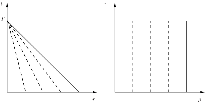
with appropriate initial data. The concrete form of the data is irrelevant for the mode analysis and therefore, we omit them in this section. Since the solution ψT\psi^{T} is self–similar, it is natural to switch to similarity coordinates (τ,ρ)(\tau,\rho) defined by τ:=−log⁡(T−t)\tau:=-\log(T-t), ρ:=rT−t\rho:=\frac{r}{T-t}.

Refer to caption
Figure 3.1. The backward lightcone 𝒞T\mathcal{C}_{T} in (t,r)(t,r) and (τ,ρ)(\tau,\rho) coordinates. We have also included some lines of constant ρ\rho (dashed).

Observe that this change of variables transforms the cone 𝒞T\mathcal{C}_{T} to the infinite cylinder

𝒵T:={(τ,ρ):τ>−logT,ρ∈[0,1]},\mathcal{Z}_{T}:=\{(\tau,\rho):\tau>-\log T,\rho\in[0,1]\},

see Fig. 3.1. In particular, the blow up of ψT\psi^{T} takes place as τ\tau goes to infinity. According to the chain rule, the derivatives transform as ∂t=eτ(∂τ+ρ∂ρ)\partial_{t}=e^{\tau}(\partial_{\tau}+\rho\partial_{\rho}) and ∂r=eτ∂ρ\partial_{r}=e^{\tau}\partial_{\rho}. In similarity coordinates (τ,ρ)(\tau,\rho), the evolution equation (3.9) reads

(3.10) ϕτ​τ+ϕτ+2​ρ​ϕτ​ρ−(1−ρ2)​ϕρ​ρ−2​1−ρ2ρ​ϕρ+V⁡(ρ)ρ2​ϕ=0\phi_{\tau\tau}+\phi_{\tau}+2\rho\phi_{\tau\rho}-(1-\rho^{2})\phi_{\rho\rho}-2\frac{1-\rho^{2}}{\rho}\phi_{\rho}+\frac{V(\rho)}{\rho^{2}}\phi=0

where ϕ⁡(τ,ρ):=φ⁡(T−e−τ,e−τ​ρ)\phi(\tau,\rho):=\varphi(T-e^{-\tau},e^{-\tau}\rho) and the “potential” VV is given by

(3.11) V⁡(ρ)=2​cos⁡(4​arctan⁡(ρ))=2​(1−6​ρ2+ρ4)(1+ρ2)2.V(\rho)=2\cos(4\arctan(\rho))=\frac{2(1-6\rho^{2}+\rho^{4})}{(1+\rho^{2})^{2}}.

The first step in a stability analysis of such an equation is to look for mode solutions, i.e., solutions of the form ϕ⁡(τ,ρ,λ)=eλ​τ​u​(ρ,λ)\phi(\tau,\rho;\lambda)=e^{\lambda\tau}u(\rho,\lambda) for a complex number λ\lambda and a sufficiently regular function u⁡(⋅,λ)u(\cdot,\lambda). The nonexistence of mode solutions with Re​λ≥0\mathrm{Re}\lambda\geq 0 is a necessary (though, in general, not sufficient) requirement for linear stability of the fundamental self–similar solution ψT\psi^{T}.

3.2. The eigenvalue equation

In order to decide whether there are unstable mode solutions or not, we insert the ansatz ϕ⁡(τ,ρ,λ)=eλ​τ​u​(ρ,λ)\phi(\tau,\rho;\lambda)=e^{\lambda\tau}u(\rho,\lambda) into Eq. (3.10) to derive the ordinary differential equation

(3.12) −(1−ρ2)​u′′​(ρ,λ)−2​1−ρ2ρ​u′​(ρ,λ)+2​λ​ρ​u′​(ρ,λ)+V⁡(ρ)ρ2​u​(ρ,λ)+λ⁡(λ+1)​u​(ρ,λ)=0-(1-\rho^{2})u^{\prime\prime}(\rho,\lambda)-2\frac{1-\rho^{2}}{\rho}u^{\prime}(\rho,\lambda)+2\lambda\rho u^{\prime}(\rho,\lambda)+\frac{V(\rho)}{\rho^{2}}u(\rho,\lambda)+\lambda(\lambda+1)u(\rho,\lambda)=0

which constitutes a generalized eigenvalue problem for the function u⁡(⋅,λ)u(\cdot,\lambda) where ′ always means derivative with respect to ρ\rho. Unfortunately, due to the complexity of the potential VV, this equation cannot be solved explicitly and it seems to be a hard problem to exclude unstable mode solutions rigorously. Indeed, there are only partial results available, see below. The rest of this section is devoted to the analysis of Eq. (3.12).

We start off with some basic observations. Eq. (3.12) has two regular singular points at ρ=0\rho=0 and ρ=1\rho=1 (which is the location of the lightcone). Furthermore, a brief inspection of the potential VV shows that additionally there are regular singular points outside the “physical” domain at ρ=−1,±i\rho=-1,\pm i as well as ρ=∞\rho=\infty. By the change of variables ρ↦ρ2\rho\mapsto\rho^{2} one can reduce the number of regular singular points from six to four which shows that the general solution is given in terms of Heun’s functions. This, however, is not of much use for us since there is no rigorous theory of Heun’s functions and most of the results are based on some sort of numerics. Nevertheless, we can at least get information on the asymptotic behavior of the solutions around the singular points ρ=0\rho=0 and ρ=1\rho=1 by applying Frobenius’ method (see e.g., [30], §6.2). The indices at ρ=0\rho=0 are {1,−2}\{1,-2\} and at ρ=1\rho=1 we have {0,1−λ}\{0,1-\lambda\} which shows that analytic solutions behave like ρ\rho around 00 and like 11 at ρ=1\rho=1. However, note carefully that the nonanalytic solution around ρ=1\rho=1 behaves like (1−ρ)1−λ(1-\rho)^{1-\lambda} and it therefore becomes more and more regular as Re​λ\mathrm{Re}\lambda decreases. It is not clear at this stage (and in fact it is false) that only analytic solutions of Eq. (3.12) are relevant. The precise regularity requirements can only be derived once one has a well–posed initial value formulation of Eq. (3.10) and a well–defined spectral problem. This will be postponed to Sec. 4 and for the moment we only look for analytic solutions of Eq. (3.12). Thus, we say that λ∈ℂ\lambda\in\mathbb{C} is an eigenvalue iff Eq. (3.12) has a nontrivial analytic solution u⁡(ρ,λ)u(\rho,\lambda). Note also that it is sufficient to consider smooth solutions (i.e., solutions in C∞​[0,1]C^{\infty}[0,1]) since any smooth solution of Eq. (3.12) is automatically analytic by Frobenius’ method.

3.3. The gauge mode

By a direct computation one immediately checks that the function g⁡(ρ)=ρ1+ρ2g(\rho)=\frac{\rho}{1+\rho^{2}} is a solution of Eq. (3.12) with λ=1\lambda=1 and thus, there exists an unstable mode. However, it is well–known that this instability emerges from the fact that ψT\psi^{T} is a family of solutions (depending on the free parameter TT) rather than a single one. Hence, the time translation symmetry of the original wave map equation (1.3) is reflected by this unstable mode of the linearized operator and therefore, the mode gg is sometimes called a gauge mode. As a consequence, we really want to study stability “modulo” this gauge instability. We will make this precise in Sec. 4. For the moment we just ignore this gauge mode and look for other unstable modes. Note also that there are no other “gauge modes” since all the remaining symmetries of the equation are eliminated by our restriction to co–rotational wave maps (of course, there is still the scaling symmetry but, when acting on a self–similar solution, scaling and time translation are equivalent).

3.4. Known results

The eigenvalue equation (3.12) has been extensively studied by several authors. First, there are a number of numerical works where essentially three different methods have been applied to show that there are no unstable modes 22 2 We always mean unstable modes apart from the gauge mode.. Probably the easiest thing to do is to employ a so–called shooting and matching technique where one integrates the equation (3.12) away from the singular points by using a standard numerical method like Runge–Kutta or variants thereof. One then tries to match the two solutions at ρ=12\rho=\frac{1}{2}. Such a numerical analysis has been performed in [10], [12], [4], [29]. Special care has to be taken since one has to solve singular initial value problems but this can be done in a satisfactory way. A more serious disadvantage of this method is that one has to have good initial guesses and therefore, it is in principle possible to “miss” eigenvalues. That is why one would like to have additional (theoretical) arguments that there are no eigenvalues far away from the real axis. In fact, we will prove such a statement, see Lemma 4.23 below. Second, one can numerically integrate the time evolution equation (3.10) and remove the gauge instability by a suitable projection [10], [12]. With this approach one cannot “miss” eigenvalues with large imaginary parts but it is numerically more delicate since one has to solve a PDE instead of an ODE. Finally, it is possible to rewrite the problem (3.12) as a difference equation and use continued fractions expansions which eventually leads to a root finding problem for a transcendental function. This is a highly accurate method and it has been successfully applied to Eq. (3.12) in [2]. The outcome of all these numerical studies is that the eigenvalue with the largest real part (apart from the gauge mode) is λ≈−0.542466\lambda\approx-0.542466 and this strongly suggests the mode stability of the solution ψT\psi^{T}.

As far as rigorous arguments are concerned, there are only partial results. In [14], Eq. (3.12) is transformed into a self–adjoint Sturm–Liouville form and this approach can be used to show that there are no unstable eigenvalues λ\lambda with Re​λ>1\mathrm{Re}\lambda>1. Furthermore, by ODE techniques it has been proved that there are no real unstable eigenvalues except for λ=1\lambda=1 [13]. However, there is no result so far that excludes unstable eigenvalues λ\lambda with 0≤Re​λ<10\leq\mathrm{Re}\lambda<1 and Im​λ≠0\mathrm{Im}\lambda\not=0. In what follows we push the boundary a bit further and prove a result that excludes eigenvalues λ\lambda with Re​λ≥12\mathrm{Re}\lambda\geq\frac{1}{2}.

3.5. The dual eigenvalue problem

In [14] there is given a factorization of the linear operator which can be used to obtain a “dual” eigenvalue problem which gives important new insights into the problem of mode stability.

Lemma 3.1.

Let u⁡(⋅,λ)∈C∞​[0,1]u(\cdot,\lambda)\in C^{\infty}[0,1] be a nontrivial solution of Eq. (3.12). Then either λ=1\lambda=1 and u⁡(ρ,1)=c​ρ1+ρ2u(\rho,1)=\frac{c\rho}{1+\rho^{2}} for a constant c∈ℂc\in\mathbb{C} (i.e., u⁡(⋅,λ)u(\cdot,\lambda) is a multiple of the gauge mode) or the equation

(3.13) −(1−ρ2)​v′′​(ρ,λ)−2​1−ρ2ρ​v′​(ρ,λ)+2​λ​ρ​v′​(ρ,λ)+V~​(ρ)ρ2​v​(ρ,λ)+λ⁡(λ+1)​v​(ρ,λ)=0,-(1-\rho^{2})v^{\prime\prime}(\rho,\lambda)-2\frac{1-\rho^{2}}{\rho}v^{\prime}(\rho,\lambda)+2\lambda\rho v^{\prime}(\rho,\lambda)+\frac{\tilde{V}(\rho)}{\rho^{2}}v(\rho,\lambda)+\lambda(\lambda+1)v(\rho,\lambda)=0,

with the potential

V~​(ρ):=6−2​ρ21+ρ2\tilde{V}(\rho):=\frac{6-2\rho^{2}}{1+\rho^{2}}

has a nontrivial solution v⁡(⋅,λ)∈C∞​[0,1]v(\cdot,\lambda)\in C^{\infty}[0,1].

Proof.

Let u⁡(⋅,λ)∈C∞​[0,1]u(\cdot,\lambda)\in C^{\infty}[0,1] be a nontrivial solution of Eq. (3.12). We define a new variable u~​(ρ,λ):=(1−ρ2)λ/2​u​(ρ,λ)\tilde{u}(\rho,\lambda):=(1-\rho^{2})^{\lambda/2}u(\rho,\lambda). Then u~​(⋅,λ)\tilde{u}(\cdot,\lambda) satisfies

−(1−ρ2)2​u~′′​(ρ,λ)−2​(1−ρ2)2ρ​u~′​(ρ,λ)+(1−ρ2)​V​(ρ)−ρ2ρ2​u~​(ρ,λ)=−(1−λ)2​u~​(ρ,λ)-(1-\rho^{2})^{2}\tilde{u}^{\prime\prime}(\rho,\lambda)-2\frac{(1-\rho^{2})^{2}}{\rho}\tilde{u}^{\prime}(\rho,\lambda)+\frac{(1-\rho^{2})V(\rho)-\rho^{2}}{\rho^{2}}\tilde{u}(\rho,\lambda)=-(1-\lambda)^{2}\tilde{u}(\rho,\lambda)

and this equation can be written as

(3.14) β^​β​u~​(⋅,λ)=−(1−λ)2​u~​(⋅,λ)\hat{\beta}\beta\tilde{u}(\cdot,\lambda)=-(1-\lambda)^{2}\tilde{u}(\cdot,\lambda)

where the (formal) differential operators β\beta and β^\hat{\beta} are given by

β:=(1−ρ2)​dd​ρ−1−3​ρ2ρ⁡(1+ρ2)\beta:=(1-\rho^{2})\frac{d}{d\rho}-\frac{1-3\rho^{2}}{\rho(1+\rho^{2})}

and

β^:=−(1−ρ2)​dd​ρ−3−ρ2ρ⁡(1+ρ2),\hat{\beta}:=-(1-\rho^{2})\frac{d}{d\rho}-\frac{3-\rho^{2}}{\rho(1+\rho^{2})},

see [14]. The solutions of the first–order ODE β​u~=0\beta\tilde{u}=0 can be given explicitly and the one–dimensional solution space is spanned by the function ρ↦ρ​1−ρ21+ρ2\rho\mapsto\frac{\rho\sqrt{1-\rho^{2}}}{1+\rho^{2}}. Thus, if β​u~​(⋅,λ)=0\beta\tilde{u}(\cdot,\lambda)=0 then Eq. (3.14) implies λ=1\lambda=1 and u⁡(⋅,λ)u(\cdot,\lambda) is a multiple of the gauge mode. Suppose β​u~​(⋅,λ)≠0\beta\tilde{u}(\cdot,\lambda)\not=0. Applying the operator β\beta to Eq. (3.14) yields

(3.15) β​β^​β​u~​(⋅,λ)=−(1−λ)2​β​u~​(⋅,λ)\beta\hat{\beta}\beta\tilde{u}(\cdot,\lambda)=-(1-\lambda)^{2}\beta\tilde{u}(\cdot,\lambda)

and this is a second order ODE for the nonzero function v~​(⋅,λ):=β​u~​(⋅,λ)\tilde{v}(\cdot,\lambda):=\beta\tilde{u}(\cdot,\lambda). The operator β\beta is singular at ρ=0\rho=0 but due to the asymptotics u~​(ρ,λ)≃ρ\tilde{u}(\rho,\lambda)\simeq\rho as ρ→0+\rho\to 0+ (Frobenius’ method) we still have v~(⋅,λ)∈C∞[0,1)\tilde{v}(\cdot,\lambda)\in C^{\infty}[0,1). Furthermore, as ρ→1−\rho\to 1-, v~​(ρ,λ)\tilde{v}(\rho,\lambda) behaves like (1−ρ)λ/2(1-\rho)^{\lambda/2}. Explicitly, Eq. (3.15) reads

−(1−ρ2)2​v~′′​(ρ,λ)−2​(1−ρ2)2ρ​v~′​(ρ,λ)+(1−ρ2)​V~​(ρ)−ρ2ρ2​v~​(ρ,λ)=−(1−λ)2​v~​(ρ,λ)-(1-\rho^{2})^{2}\tilde{v}^{\prime\prime}(\rho,\lambda)-2\frac{(1-\rho^{2})^{2}}{\rho}\tilde{v}^{\prime}(\rho,\lambda)+\frac{(1-\rho^{2})\tilde{V}(\rho)-\rho^{2}}{\rho^{2}}\tilde{v}(\rho,\lambda)=-(1-\lambda)^{2}\tilde{v}(\rho,\lambda)

with the new potential V~​(ρ)=6−2​ρ21+ρ2\tilde{V}(\rho)=\frac{6-2\rho^{2}}{1+\rho^{2}}. Setting v(ρ,λ):=(1−ρ2)−λ/2v~(ρ,λ)v(\rho,\lambda):=(1-\rho^{2})^{-\lambda/2}\tilde{v}(\rho,\lambda) we obtain v⁡(⋅,λ)∈C∞​[0,1]v(\cdot,\lambda)\in C^{\infty}[0,1] and v⁡(⋅,λ)v(\cdot,\lambda) satisfies Eq. (3.13). ∎

3.6. Nonexistence of eigenvalues with Re​λ≥12\mathrm{Re}\lambda\geq\frac{1}{2}

Based on Lemma 3.1 we can now prove that the gauge mode is the only eigenmode with Re​λ≥12\mathrm{Re}\lambda\geq\frac{1}{2}.

Proposition 3.2.

Let u⁡(⋅,λ)∈C∞​[0,1]u(\cdot,\lambda)\in C^{\infty}[0,1] be a nontrivial solution of Eq. (3.12) with Re​λ≥12\mathrm{Re}\lambda\geq\frac{1}{2}. Then λ=1\lambda=1 and there exists a (nonzero) constant c∈ℂc\in\mathbb{C} such that u⁡(ρ,1)=c​ρ1+ρ2u(\rho,1)=\frac{c\rho}{1+\rho^{2}}.

Proof.

Let u⁡(⋅,λ)∈C∞​[0,1]u(\cdot,\lambda)\in C^{\infty}[0,1] be a nonzero solution of Eq. (3.12) with Re≥12\mathrm{Re}\geq\frac{1}{2} and assume that λ≠1\lambda\not=1. According to Lemma 3.1 there exists a nonzero v⁡(⋅,λ)∈C∞​[0,1]v(\cdot,\lambda)\in C^{\infty}[0,1] such that

−(1−ρ2)​v′′​(ρ,λ)−2​1−ρ2ρ​v′​(ρ,λ)+2​λ​ρ​v′​(ρ,λ)+V~​(ρ)ρ2​v​(ρ,λ)+λ⁡(λ+1)​v​(ρ,λ)=0.-(1-\rho^{2})v^{\prime\prime}(\rho,\lambda)-2\frac{1-\rho^{2}}{\rho}v^{\prime}(\rho,\lambda)+2\lambda\rho v^{\prime}(\rho,\lambda)+\frac{\tilde{V}(\rho)}{\rho^{2}}v(\rho,\lambda)+\lambda(\lambda+1)v(\rho,\lambda)=0.

Thus, χ⁡(τ,ρ,λ):=eλ​τ​v​(ρ,λ)\chi(\tau,\rho;\lambda):=e^{\lambda\tau}v(\rho,\lambda) is a smooth solution of the evolution equation

χτ​τ+χτ+2​ρ​χτ​ρ−(1−ρ2)​χρ​ρ−2​1−ρ2ρ​χρ+V~​(ρ)ρ2​χ=0\chi_{\tau\tau}+\chi_{\tau}+2\rho\chi_{\tau\rho}-(1-\rho^{2})\chi_{\rho\rho}-2\frac{1-\rho^{2}}{\rho}\chi_{\rho}+\frac{\tilde{V}(\rho)}{\rho^{2}}\chi=0

and transforming back to the physical coordinates (t,r)(t,r) this simply reads

χt​t−χr​r−2r​χr+V~​(rT−t)r2​χ=0.\chi_{tt}-\chi_{rr}-\frac{2}{r}\chi_{r}+\frac{\tilde{V}(\frac{r}{T-t})}{r^{2}}\chi=0.

Motivated by the energy of this equation, consider the positive smooth function

Fχ​(t):=12​∫0T−t[r2​|χt​(t,r,λ)|2+r2​|χr​(t,r,λ)|2+V~​(rT−t)​|χ⁡(t,r,λ)|2]​𝑑r.F_{\chi}(t):=\frac{1}{2}\int_{0}^{T-t}\left[r^{2}|\chi_{t}(t,r;\lambda)|^{2}+r^{2}|\chi_{r}(t,r;\lambda)|^{2}+\tilde{V}\left(\frac{r}{T-t}\right)|\chi(t,r;\lambda)|^{2}\right]dr.

Differentiation yields

Fχ′​(t)\displaystyle F_{\chi}^{\prime}(t) =Re​∫0T−t[r2​χt​t​χt¯+r2​χr​χr​t¯+V~​(rT−t)​χ​χt¯+12​V~′​(rT−t)⏟≤0​r(T−t)2​|χ|2​𝑑r]\displaystyle=\mathrm{Re}\int_{0}^{T-t}\left[r^{2}\chi_{tt}\overline{\chi_{t}}+r^{2}\chi_{r}\overline{\chi_{rt}}+\tilde{V}\left(\frac{r}{T-t}\right)\chi\overline{\chi_{t}}+\frac{1}{2}\underbrace{\tilde{V}^{\prime}\left(\frac{r}{T-t}\right)}_{\leq 0}\frac{r}{(T-t)^{2}}|\chi|^{2}dr\right]
−12​(T−t)2​|χt​(t,T−t,λ)|2−12​(T−t)2​|χr​(t,T−t,λ)|2−12​V~​(1)​|χ⁡(t,T−t,λ)|2\displaystyle\quad-\frac{1}{2}(T-t)^{2}|\chi_{t}(t,T-t;\lambda)|^{2}-\frac{1}{2}(T-t)^{2}|\chi_{r}(t,T-t;\lambda)|^{2}-\frac{1}{2}\tilde{V}(1)|\chi(t,T-t;\lambda)|^{2}
≤Re​∫0T−t[∂r(r2​χr)​χt¯+r2​χr​χr​t¯]​𝑑r\displaystyle\leq\mathrm{Re}\int_{0}^{T-t}\left[\partial_{r}(r^{2}\chi_{r})\overline{\chi_{t}}+r^{2}\chi_{r}\overline{\chi_{rt}}\right]dr
−12​(T−t)2​|χt​(t,T−t,λ)|2−12​(T−t)2​|χr​(t,T−t,λ)|2−12​V~​(1)​|χ⁡(t,T−t,λ)|2\displaystyle\quad-\frac{1}{2}(T-t)^{2}|\chi_{t}(t,T-t;\lambda)|^{2}-\frac{1}{2}(T-t)^{2}|\chi_{r}(t,T-t;\lambda)|^{2}-\frac{1}{2}\tilde{V}(1)|\chi(t,T-t;\lambda)|^{2}
≤−|χ⁡(t,T−t,λ)|2\displaystyle\leq-|\chi(t,T-t;\lambda)|^{2}

by integration by parts and Cauchy’s inequality. Inserting χ⁡(t,T−t,λ)=(T−t)−λ​v​(1)\chi(t,T-t;\lambda)=(T-t)^{-\lambda}v(1) and integrating from 00 to tt for t<Tt<T yields

Fχ(t)≤−|v(1)|2∫0t(T−t′)−2​R​e​λdt′+Fχ(0).F_{\chi}(t)\leq-|v(1)|^{2}\int_{0}^{t}(T-t^{\prime})^{-2\mathrm{Re}\lambda}dt^{\prime}+F_{\chi}(0).

However, from the asymptotic behavior of vv we know that v⁡(1)≠0v(1)\not=0 and therefore we have a contradiction since FχF_{\chi} is positive but the right–hand side of the above inequality goes to −∞-\infty as t→T−t\to T- (recall that we assume Re​λ≥12\mathrm{Re}\lambda\geq\frac{1}{2}). ∎

3.7. Reformulation as a resonance problem

We conclude this section by showing that the mode stability problem is in fact equivalent to finding resonances of the ℓ=2\ell=2 Schrödinger operator with a potential that has inverse square decay towards infinity. We formulate the problem for the “dual” eigenvalue equation

−(1−ρ2)​v′′​(ρ,λ)−2​1−ρ2ρ​v′​(ρ,λ)+2​λ​ρ​v′​(ρ,λ)+V~​(ρ)ρ2​v​(ρ,λ)+λ⁡(λ+1)​v​(ρ,λ)=0-(1-\rho^{2})v^{\prime\prime}(\rho,\lambda)-2\frac{1-\rho^{2}}{\rho}v^{\prime}(\rho,\lambda)+2\lambda\rho v^{\prime}(\rho,\lambda)+\frac{\tilde{V}(\rho)}{\rho^{2}}v(\rho,\lambda)+\lambda(\lambda+1)v(\rho,\lambda)=0

with potential V~​(ρ)=6−2​ρ21+ρ2\tilde{V}(\rho)=\frac{6-2\rho^{2}}{1+\rho^{2}}. We are interested in smooth solutions and according to numerics we expect the eigenvalue with the largest real part to be λ≈−0.54\lambda\approx-0.54. Now suppose v⁡(⋅,λ)v(\cdot,\lambda) is an eigenfunction, i.e., a smooth solution to the above equation. By Frobenius’ method we have the asymptotic behavior v⁡(ρ,λ)≃ρ2v(\rho,\lambda)\simeq\rho^{2} as ρ→0+\rho\to 0+ and v⁡(ρ,λ)≃1v(\rho,\lambda)\simeq 1 as ρ→1−\rho\to 1-. Defining a new variable v~\tilde{v} by

v~​(x,μ):=(1−tanh2⁡x)λ/2​sinh⁡x​u​(tanh⁡x,1−i​μ),\tilde{v}(x,\mu):=(1-\tanh^{2}x)^{\lambda/2}\sinh x\>u(\tanh x,1-i\mu),

the eigenvalue problem transforms into

(3.16) −v~′′​(x,λ)+6x2​v~​(x,λ)+Q⁡(x)​v~​(x,λ)=μ2​v~​(x,λ)-\tilde{v}^{\prime\prime}(x,\lambda)+\frac{6}{x^{2}}\tilde{v}(x,\lambda)+Q(x)\tilde{v}(x,\lambda)=\mu^{2}\tilde{v}(x,\lambda)

on the half–line x≥0x\geq 0 with the potential

Q⁡(x)=V~​(tanh⁡x)sinh2⁡x−6x2.Q(x)=\frac{\tilde{V}(\tanh x)}{\sinh^{2}x}-\frac{6}{x^{2}}.

The outgoing Jost solution f+​(⋅,μ)f_{+}(\cdot,\mu) is defined as the solution of Eq. (3.16) that behaves like f+​(x,μ)∼ei​μ​xf_{+}(x,\mu)\sim e^{i\mu x} as x→∞x\to\infty. Furthermore, we denote by f0​(⋅,μ)f_{0}(\cdot,\mu) the solution of Eq. (3.16) which is square–integrable near x=0x=0. The eigenfunction v~​(⋅,μ)\tilde{v}(\cdot,\mu) has the asymptotic behavior v~​(x,μ)≃x3\tilde{v}(x,\mu)\simeq x^{3} as x→0+x\to 0+ and v~​(x,μ)≃ei​μ​x\tilde{v}(x,\mu)\simeq e^{i\mu x} as x→∞x\to\infty. Thus, finding eigenvalues amounts to matching the outgoing Jost solution f+​(⋅,μ)f_{+}(\cdot,\mu) to f0​(⋅,μ)f_{0}(\cdot,\mu) or, in other words, λ\lambda is an eigenvalue iff μ=i⁡(λ−1)\mu=i(\lambda-1) is a zero of the Wronskian

W⁡(f0,f+)​(μ)=f0​(⋅,μ)​f+′​(⋅,μ)−f0′​(⋅,μ)​f+​(⋅,μ).W(f_{0},f_{+})(\mu)=f_{0}(\cdot,\mu)f_{+}^{\prime}(\cdot,\mu)-f_{0}^{\prime}(\cdot,\mu)f_{+}(\cdot,\mu).

We are mainly interested in eigenvalues λ\lambda with Re​λ<1\mathrm{Re}\lambda<1 and this translates into the condition Im​μ<0\mathrm{Im}\mu<0 since μ=−Im​λ+i​Re​(λ−1)\mu=-\mathrm{Im}\lambda+i\mathrm{Re}(\lambda-1). However, zeros of the Wronskian W⁡(f0,f+)​(μ)W(f_{0},f_{+})(\mu) with Im​μ<0\mathrm{Im}\mu<0 are precisely the resonances or scattering poles of the Schrödinger operator defined by Eq. (3.16).

4. The linear perturbation theory

4.1. First–order formulation

We intend to rewrite the wave maps equation (2.5) as a system which is first–order in time. From now on we are a bit more careful and specify the full Cauchy problem we want to study, including the initial data and the domain. Recall the definition of the backward lightcone

𝒞T:={(t,r):t∈(0,T),r∈[0,T−t]}.\mathcal{C}_{T}:=\{(t,r):t\in(0,T),r\in[0,T-t]\}.

Precisely, we are interested in the evolution problem

(4.17) {ψt​t​(t,r)−ψr​r​(t,r)−2r​ψr​(t,r)+sin⁡(2​ψ​(t,r))r2=0​ for ​(t,r)∈𝒞Tψ⁡(0,r)=f⁡(r),ψt​(0,r)=g⁡(r)​ for ​r∈[0,T]\left\{\begin{array}[]{l}\psi_{tt}(t,r)-\psi_{rr}(t,r)-\frac{2}{r}\psi_{r}(t,r)+\frac{\sin(2\psi(t,r))}{r^{2}}=0\mbox{ for }(t,r)\in\mathcal{C}_{T}\\ \psi(0,r)=f(r),\psi_{t}(0,r)=g(r)\mbox{ for }r\in[0,T]\end{array}\right.

with given initial data (f,g)(f,g). For the remainder of this section we assume that a solution ψ\psi of the Cauchy problem (4.17) exists and it is sufficiently regular so that all of the following computations are justified. In particular, we assume that ψ\psi satisfies the regularity condition ψ⁡(t,0)=0\psi(t,0)=0 which implies f⁡(0)=g⁡(0)=0f(0)=g(0)=0. Actually, we want to study the flow about the self–similar solution ψT\psi^{T} and thus, we are interested in “small” perturbations φ\varphi of ψT\psi^{T}. Thus, it is convenient to rewrite the problem relative to ψT\psi^{T} by setting ψ=ψT+φ\psi=\psi^{T}+\varphi and expanding the nonlinearity in Eq. (4.17) as

sin⁡(2​(ψT+φ))=sin⁡(2​ψT)+2​cos⁡(2​ψT)​φ+NT​(φ)\sin(2(\psi^{T}+\varphi))=\sin(2\psi^{T})+2\cos(2\psi^{T})\varphi+N_{T}(\varphi)

where NT​(x)=O⁡(x2)N_{T}(x)=O(x^{2}) for x→0x\to 0 is the nonlinear remainder. The Cauchy problem (4.17) becomes

(4.18) {φt​t−φr​r−2r​φr+2r2​φ+2​cos⁡(2​ψT)−2r2​φ+NT​(φ)r2=0​ in ​𝒞Tφ⁡(0,r)=f⁡(r)−ψT​(0,r),φt​(0,r)=g⁡(r)−ψtT​(0,r)​ for ​r∈[0,T]\left\{\begin{array}[]{l}\varphi_{tt}-\varphi_{rr}-\frac{2}{r}\varphi_{r}+\frac{2}{r^{2}}\varphi+\frac{2\cos(2\psi^{T})-2}{r^{2}}\varphi+\frac{N_{T}(\varphi)}{r^{2}}=0\mbox{ in }\mathcal{C}_{T}\\ \varphi(0,r)=f(r)-\psi^{T}(0,r),\varphi_{t}(0,r)=g(r)-\psi^{T}_{t}(0,r)\mbox{ for }r\in[0,T]\end{array}\right.

where we have suppressed the arguments of φ\varphi and ψT\psi^{T} so as not to overload the equation with too many symbols. From the regularity requirement ψ⁡(t,0)=0\psi(t,0)=0 we obtain the boundary condition φ⁡(t,0)=0\varphi(t,0)=0 for all t∈[0,T)t\in[0,T). Next, motivated by the discussion in Sec. 2, we introduce the new variable φ~​(t,r):=r2​φ​(t,r)\tilde{\varphi}(t,r):=r^{2}\varphi(t,r) which yields

(4.19) {φ~t​t−φ~r​r+2r​φ~r+2​cos⁡(2​ψT)−2r2​φ~+NT​(r−2​φ~)=0​ in ​𝒞Tφ~​(0,r)=r2​[f⁡(r)−ψT​(0,r)],φ~t​(0,r)=r2​[g⁡(r)−ψtT​(0,r)]​ for ​r∈[0,T]\left\{\begin{array}[]{l}\tilde{\varphi}_{tt}-\tilde{\varphi}_{rr}+\frac{2}{r}\tilde{\varphi}_{r}+\frac{2\cos(2\psi^{T})-2}{r^{2}}\tilde{\varphi}+N_{T}(r^{-2}\tilde{\varphi})=0\mbox{ in }\mathcal{C}_{T}\\ \tilde{\varphi}(0,r)=r^{2}[f(r)-\psi^{T}(0,r)],\tilde{\varphi}_{t}(0,r)=r^{2}[g(r)-\psi^{T}_{t}(0,r)]\mbox{ for }r\in[0,T]\end{array}\right.

and again, we occasionally omit the arguments of φ~\tilde{\varphi} and ψT\psi^{T}. In order to write this Cauchy problem as a first–order system in time, we introduce the variables

φ1​(t,r):=φ~t​(t,r)T−t,φ2​(t,r):=φ~r​(t,r)r.\varphi_{1}(t,r):=\frac{\tilde{\varphi}_{t}(t,r)}{T-t},\quad\varphi_{2}(t,r):=\frac{\tilde{\varphi}_{r}(t,r)}{r}.

This choice is motivated by the fact that φj\varphi_{j}, j=1,2j=1,2, scale like the original field φ\varphi or, in other words, they have the same physical dimension. Furthermore, the higher energy (2.8) is a simple expression in terms of φj\varphi_{j}. Note also that the field φ~\tilde{\varphi} can be reconstructed from φ2\varphi_{2} by

φ~​(t,r)=∫0rr′​φ2​(t,r′)​d​r′\tilde{\varphi}(t,r)=\int_{0}^{r}r^{\prime}\varphi_{2}(t,r^{\prime})dr^{\prime}

thanks to the boundary condition φ~​(t,0)=0\tilde{\varphi}(t,0)=0 for all t∈[0,T)t\in[0,T). We obtain the system

(4.20) {∂tφ1=(T−t)−1​[φ1+r​∂rφ2−φ2−2​cos⁡(2​ψT)−2r2​∫r​φ2−NT​(r−2​∫r​φ2)]∂tφ2=T−tr​∂rφ1}​ in ​𝒞Tφ1​(0,r)=1T​r2​[g⁡(r)−ψtT​(0,r)]φ2​(0,r)=r−1​∂rr2​[f⁡(r)−ψT​(0,r)]}​ for ​r∈[0,T]\left\{\begin{array}[]{l}\left.\begin{array}[]{l}\partial_{t}\varphi_{1}=(T-t)^{-1}\left[\varphi_{1}+r\partial_{r}\varphi_{2}-\varphi_{2}-\frac{2\cos(2\psi^{T})-2}{r^{2}}\int r\varphi_{2}-N_{T}\left(r^{-2}\int r\varphi_{2}\right)\right]\\ \partial_{t}\varphi_{2}=\frac{T-t}{r}\partial_{r}\varphi_{1}\end{array}\right\}\mbox{ in }\mathcal{C}_{T}\\ \left.\begin{array}[]{l}\varphi_{1}(0,r)=\frac{1}{T}r^{2}\left[g(r)-\psi^{T}_{t}(0,r)\right]\\ \varphi_{2}(0,r)=r^{-1}\partial_{r}r^{2}\left[f(r)-\psi^{T}(0,r)\right]\end{array}\right\}\mbox{ for }r\in[0,T]\end{array}\right.

where ∫r​φ2\int r\varphi_{2} is shorthand for ∫0rr′​φ2​(t,r′)​d​r′\int_{0}^{r}r^{\prime}\varphi_{2}(t,r^{\prime})dr^{\prime}. Now we switch to similarity coordinates

τ=−log⁡(T−t),ρ=rT−t.\tau=-\log(T-t),\quad\rho=\tfrac{r}{T-t}.

Then we have

∫0rr′​φ2​(t,r′)​d​r′=e−2​τ​∫0ρρ′​φ2​(t,e−τ​ρ′)​d​ρ′\int_{0}^{r}r^{\prime}\varphi_{2}(t,r^{\prime})dr^{\prime}=e^{-2\tau}\int_{0}^{\rho}\rho^{\prime}\varphi_{2}(t,e^{-\tau}\rho^{\prime})d\rho^{\prime}

and t=0t=0 corresponds to τ=−log⁡T\tau=-\log T. Thus, the system (4.20) transforms into

(4.21) {∂τϕ1=−ρ∂ρϕ1+ϕ1+ρ∂ρϕ2−ϕ2−2​cos⁡(2​f0)−2ρ2∫ρϕ2−NT(ρ−2∫ρϕ2)∂τϕ2=1ρ​∂ρϕ1−ρ​∂ρϕ2}​ in ​𝒵Tϕ1​(−log⁡T,ρ)=T​ρ2​[g⁡(T​ρ)−ψtT​(0,T​ρ)]ϕ2​(−log⁡T,ρ)=T​ρ​[f′​(T​ρ)−ψrT​(0,T​ρ)]+2​[f⁡(T​ρ)−ψT​(0,T​ρ)]}​ for ​ρ∈[0,1]\left\{\begin{array}[]{l}\left.\begin{array}[]{l}\partial_{\tau}\phi_{1}=-\rho\partial_{\rho}\phi_{1}+\phi_{1}+\rho\partial_{\rho}\phi_{2}-\phi_{2}-\frac{2\cos(2f_{0})-2}{\rho^{2}}\int\rho\phi_{2}-N_{T}\left(\rho^{-2}\int\rho\phi_{2}\right)\\ \partial_{\tau}\phi_{2}=\frac{1}{\rho}\partial_{\rho}\phi_{1}-\rho\partial_{\rho}\phi_{2}\end{array}\right\}\mbox{ in }\mathcal{Z}_{T}\\ \left.\begin{array}[]{l}\phi_{1}(-\log T,\rho)=T\rho^{2}\left[g(T\rho)-\psi^{T}_{t}(0,T\rho)\right]\\ \phi_{2}(-\log T,\rho)=T\rho\left[f^{\prime}(T\rho)-\psi^{T}_{r}(0,T\rho)\right]+2\left[f(T\rho)-\psi^{T}(0,T\rho)\right]\end{array}\right\}\mbox{ for }\rho\in[0,1]\end{array}\right.

where ϕj​(τ,ρ):=φj​(T−e−τ,e−τ​ρ)\phi_{j}(\tau,\rho):=\varphi_{j}(T-e^{-\tau},e^{-\tau}\rho), j=1,2j=1,2 and f0​(ρ)=2​arctan⁡(ρ)f_{0}(\rho)=2\arctan(\rho) is the fundamental self–similar solution in similarity coordinates. Tracing back the above transformations, we see that (ϕ1,ϕ2)(\phi_{1},\phi_{2}) is a (sufficiently regular) solution of (4.21) if and only if ψ\psi given by

ψ⁡(t,r)=ψT​(t,r)+1r2​∫0rr′​ϕ2​(−log⁡(T−t),r′T−t)​d​r′\psi(t,r)=\psi^{T}(t,r)+\frac{1}{r^{2}}\int_{0}^{r}r^{\prime}\phi_{2}\left(-\log(T-t),\tfrac{r^{\prime}}{T-t}\right)dr^{\prime}

is a (sufficiently regular) solution of (4.17). From now on we restrict ourselves to the linearized problem, i.e., we drop the nonlinearity in Eq. (4.21) and consider the system

(4.22) {∂τϕ1=−ρ∂ρϕ1+ϕ1+ρ∂ρϕ2−ϕ2−2​cos⁡(2​f0)−2ρ2∫ρϕ2∂τϕ2=1ρ​∂ρϕ1−ρ​∂ρϕ2}​ in ​𝒵Tϕ1​(−log⁡T,ρ)=T​ρ2​[g⁡(T​ρ)−ψtT​(0,T​ρ)]ϕ2​(−log⁡T,ρ)=T​ρ​[f′​(T​ρ)−ψrT​(0,T​ρ)]+2​[f⁡(T​ρ)−ψT​(0,T​ρ)]}​ for ​ρ∈[0,1]\left\{\begin{array}[]{l}\left.\begin{array}[]{l}\partial_{\tau}\phi_{1}=-\rho\partial_{\rho}\phi_{1}+\phi_{1}+\rho\partial_{\rho}\phi_{2}-\phi_{2}-\frac{2\cos(2f_{0})-2}{\rho^{2}}\int\rho\phi_{2}\\ \partial_{\tau}\phi_{2}=\frac{1}{\rho}\partial_{\rho}\phi_{1}-\rho\partial_{\rho}\phi_{2}\end{array}\right\}\mbox{ in }\mathcal{Z}_{T}\\ \left.\begin{array}[]{l}\phi_{1}(-\log T,\rho)=T\rho^{2}\left[g(T\rho)-\psi^{T}_{t}(0,T\rho)\right]\\ \phi_{2}(-\log T,\rho)=T\rho\left[f^{\prime}(T\rho)-\psi^{T}_{r}(0,T\rho)\right]+2\left[f(T\rho)-\psi^{T}(0,T\rho)\right]\end{array}\right\}\mbox{ for }\rho\in[0,1]\end{array}\right.

Our aim is to study Eq. (4.22) by means of semigroup theory, i.e., we rewrite the problem as an ordinary differential equation on a suitable Hilbert space.

4.2. Function spaces and operator formulation

We set

H~1:={u∈C2​[0,1]:u⁡(0)=u′​(0)=0},H~2:={u∈C1​[0,1]:u⁡(0)=0}\tilde{H}_{1}:=\{u\in C^{2}[0,1]:u(0)=u^{\prime}(0)=0\},\quad\tilde{H}_{2}:=\{u\in C^{1}[0,1]:u(0)=0\}

and define two sesquilinear forms (⋅|⋅)1(\cdot|\cdot)_{1}, (⋅|⋅)2(\cdot|\cdot)_{2} by

(u|v)1:=∫01u′​(ρ)​v′​(ρ)¯​d​ρρ2,(u|v)2:=∫01u′​(ρ)​v′​(ρ)¯​𝑑ρ.(u|v)_{1}:=\int_{0}^{1}u^{\prime}(\rho)\overline{v^{\prime}(\rho)}\frac{d\rho}{\rho^{2}},\quad(u|v)_{2}:=\int_{0}^{1}u^{\prime}(\rho)\overline{v^{\prime}(\rho)}d\rho.
Lemma 4.1.

The sesquilinear form (⋅|⋅)j(\cdot|\cdot)_{j} defines an inner product on H~j\tilde{H}_{j}, j=1,2j=1,2.

Proof.

Obviously, (⋅|⋅)2(\cdot|\cdot)_{2} is well–defined on all of H~2×H~2\tilde{H}_{2}\times\tilde{H}_{2}. Furthermore, for u∈H~2u\in\tilde{H}_{2}, (u|u)2=0(u|u)_{2}=0 is equivalent to u′=0u^{\prime}=0 which, in turn, is equivalent to u=0u=0 thanks to the boundary condition u⁡(0)=0u(0)=0. This proves the assertion for j=2j=2. For j=1j=1 we apply Hardy’s inequality to see that

(u|u)1=∫01|u′​(ρ)|2ρ2​𝑑ρ≲∫01|u′′​(ρ)|2​𝑑ρ<∞(u|u)_{1}=\int_{0}^{1}\frac{|u^{\prime}(\rho)|^{2}}{\rho^{2}}d\rho\lesssim\int_{0}^{1}|u^{\prime\prime}(\rho)|^{2}d\rho<\infty

for u∈H~1u\in\tilde{H}_{1} which is justified by the boundary condition u′​(0)=0u^{\prime}(0)=0. As a consequence, (⋅|⋅)1(\cdot|\cdot)_{1} is well–defined on all of H~1×H~1\tilde{H}_{1}\times\tilde{H}_{1}. The rest of the proof is identical to the case j=2j=2 from above. ∎

As usual, the inner product on H~j\tilde{H}_{j} induces a norm ∥⋅∥j:=(⋅|⋅)j\|\cdot\|_{j}:=\sqrt{(\cdot|\cdot)_{j}}, j=1,2j=1,2. Moreover, we denote by (⋅|⋅)(\cdot|\cdot) the canonically induced inner product on ℋ~:=H~1×H~2\tilde{\mathcal{H}}:=\tilde{H}_{1}\times\tilde{H}_{2}, i.e.,

(𝐮|𝐯):=(u1|v1)1+(u2|v2)2(\mathbf{u}|\mathbf{v}):=(u_{1}|v_{1})_{1}+(u_{2}|v_{2})_{2}

and ∥⋅∥:=(⋅|⋅)\|\cdot\|:=\sqrt{(\cdot|\cdot)}. The vector space ℋ~\tilde{\mathcal{H}} equipped with (⋅|⋅)(\cdot|\cdot) is a pre–Hilbert space and we denote by ℋ=H1×H2\mathcal{H}=H_{1}\times H_{2} its completion. We have the following convenient density result.

Lemma 4.2.

The set Cc∞(0,1]={u∈C∞[0,1]:supp(u)⊂(0,1]}C_{c}^{\infty}(0,1]=\{u\in C^{\infty}[0,1]:\mathrm{supp}(u)\subset(0,1]\} is dense in HjH_{j}, j=1,2j=1,2.

Proof.

Let u∈H~1u\in\tilde{H}_{1}. By definition, this implies u′w∈L2​(0,1)\frac{u^{\prime}}{w}\in L^{2}(0,1) where w⁡(ρ):=ρw(\rho):=\rho. It is well–known that Cc∞​(0,1)C^{\infty}_{c}(0,1) is dense in L2​(0,1)L^{2}(0,1) (see e.g., [1], p. 31, Theorem 2.19) and thus, for any given ε>0\varepsilon>0, there exists a v∈Cc∞​(0,1)v\in C^{\infty}_{c}(0,1) such that ‖u′w−v‖L2​(0,1)<ε\|\frac{u^{\prime}}{w}-v\|_{L^{2}(0,1)}<\varepsilon. Set

u~​(ρ):=∫0ρρ′​v​(ρ′)​d​ρ′.\tilde{u}(\rho):=\int_{0}^{\rho}\rho^{\prime}v(\rho^{\prime})d\rho^{\prime}.

Then u~∈Cc∞(0,1]\tilde{u}\in C^{\infty}_{c}(0,1] and u~′​(ρ)ρ=v⁡(ρ)\frac{\tilde{u}^{\prime}(\rho)}{\rho}=v(\rho). Consequently, we obtain ‖u−u~‖1=‖u′w−v‖L2​(0,1)<ε\|u-\tilde{u}\|_{1}=\|\frac{u^{\prime}}{w}-v\|_{L^{2}(0,1)}<\varepsilon and, since H~1\tilde{H}_{1} is dense in H1H_{1} by construction, this implies the claim for H1H_{1}. The proof for H2H_{2} is analogous. ∎

For later reference it is useful to note the following embedding and the fact that the boundary conditions for the functions “survive” the completion procedure.

Lemma 4.3.

We have the embedding ℋ↪C⁡[0,1]×C⁡[0,1]\mathcal{H}\hookrightarrow C[0,1]\times C[0,1] and 𝐮∈ℋ\mathbf{u}\in\mathcal{H} implies 𝐮⁡(0)=0\mathbf{u}(0)=0.

Proof.

Note first that for u∈H~2u\in\tilde{H}_{2} we have

|u⁡(ρ)|=|∫0ρu′​(ρ)​𝑑ρ|≤∫01|u′​(ρ)|​𝑑ρ≤(∫01|u′​(ρ)|2​𝑑ρ)1/2=‖u′‖L2​(0,1)=‖u‖2|u(\rho)|=\left|\int_{0}^{\rho}u^{\prime}(\rho)d\rho\right|\leq\int_{0}^{1}|u^{\prime}(\rho)|d\rho\leq\left(\int_{0}^{1}|u^{\prime}(\rho)|^{2}d\rho\right)^{1/2}=\|u^{\prime}\|_{L^{2}(0,1)}=\|u\|_{2}

for all ρ∈[0,1]\rho\in[0,1] and this computation also implies |u⁡(ρ)|≤‖u‖1|u(\rho)|\leq\|u\|_{1} for all u∈H~1u\in\tilde{H}_{1} and ρ∈[0,1]\rho\in[0,1]. By approximation, these estimates extend to H2H_{2} and H1H_{1}, respectively, and we obtain

‖𝐮‖L∞​(0,1)×L∞​(0,1)2=‖u1‖L∞​(0,1)2+‖u2‖L∞​(0,1)2≤‖𝐮‖2\|\mathbf{u}\|_{L^{\infty}(0,1)\times L^{\infty}(0,1)}^{2}=\|u_{1}\|_{L^{\infty}(0,1)}^{2}+\|u_{2}\|_{L^{\infty}(0,1)}^{2}\leq\|\mathbf{u}\|^{2}

for all 𝐮∈ℋ\mathbf{u}\in\mathcal{H} by taking the supremum over ρ∈[0,1]\rho\in[0,1]. Now let 𝐮∈ℋ\mathbf{u}\in\mathcal{H} be arbitrary. By construction, there exists a sequence (𝐮j)⊂ℋ~(\mathbf{u}_{j})\subset\tilde{\mathcal{H}} such that ‖𝐮−𝐮j‖→0\|\mathbf{u}-\mathbf{u}_{j}\|\to 0 as j→∞j\to\infty. The above inequality implies

‖𝐮−𝐮j‖L∞​(0,1)×L∞​(0,1)≲‖𝐮−𝐮j‖→0\|\mathbf{u}-\mathbf{u}_{j}\|_{L^{\infty}(0,1)\times L^{\infty}(0,1)}\lesssim\|\mathbf{u}-\mathbf{u}_{j}\|\to 0

as j→∞j\to\infty and, since the uniform limit of continuous functions is continuous, this shows that 𝐮∈C⁡[0,1]×C⁡[0,1]\mathbf{u}\in C[0,1]\times C[0,1]. In particular, 𝐮j→𝐮\mathbf{u}_{j}\to\mathbf{u} pointwise and, since 𝐮j​(0)=0\mathbf{u}_{j}(0)=0 for all jj, we obtain 𝐮⁡(0)=0\mathbf{u}(0)=0. ∎

Now we define a linear operator L~0:𝒟⁡(L~0)⊂ℋ→ℋ\tilde{L}_{0}:\mathcal{D}(\tilde{L}_{0})\subset\mathcal{H}\to\mathcal{H} that represents the spatial differential operator in Eq. (4.22) as follows. We set

𝒟⁡(L~0):={u∈C3​[0,1]:u⁡(0)=u′​(0)=u′′​(0)=0}×{u∈C3​[0,1]:u⁡(0)=0}\mathcal{D}(\tilde{L}_{0}):=\{u\in C^{3}[0,1]:u(0)=u^{\prime}(0)=u^{\prime\prime}(0)=0\}\times\{u\in C^{3}[0,1]:u(0)=0\}

and

L~0​𝐮​(ρ):=(−ρ​u1′​(ρ)+u1​(ρ)+ρ​u2′​(ρ)−u2​(ρ)1ρ​u1′​(ρ)−ρ​u2′​(ρ)).\tilde{L}_{0}\mathbf{u}(\rho):=\left(\begin{array}[]{c}-\rho u_{1}^{\prime}(\rho)+u_{1}(\rho)+\rho u_{2}^{\prime}(\rho)-u_{2}(\rho)\\ \frac{1}{\rho}u_{1}^{\prime}(\rho)-\rho u_{2}^{\prime}(\rho)\end{array}\right).

It should be emphasized that the definition of 𝒟⁡(L~0)\mathcal{D}(\tilde{L}_{0}) is a crucial point in the whole construction. One has to be very careful with the boundary conditions so as not to “lose” solutions one is actually interested in. To see that this is not the case, recall that, in terms of the original perturbation φ\varphi, the field φ1\varphi_{1} is given by

φ1​(t,r)=φ~t​(t,r)T−t=r2​φt​(t,r)T−t\varphi_{1}(t,r)=\frac{\tilde{\varphi}_{t}(t,r)}{T-t}=\frac{r^{2}\varphi_{t}(t,r)}{T-t}

and by regularity, we may assume that φt​(t,r)=O⁡(r)\varphi_{t}(t,r)=O(r) as r→0+r\to 0+. Since ϕ1\phi_{1} is nothing but φ1\varphi_{1} in similarity coordinates, we may assume ϕ1​(τ,ρ)=O⁡(ρ3)\phi_{1}(\tau,\rho)=O(\rho^{3}) as ρ→0+\rho\to 0+. Analogously, one obtains ϕ2​(τ,ρ)=O⁡(ρ)\phi_{2}(\tau,\rho)=O(\rho) as ρ→0+\rho\to 0+. This justifies the chosen boundary conditions.

Lemma 4.4.

For any 𝐮∈𝒟⁡(L~0)\mathbf{u}\in\mathcal{D}(\tilde{L}_{0}) we have L~0​𝐮∈ℋ~\tilde{L}_{0}\mathbf{u}\in\tilde{\mathcal{H}}.

Proof.

Let 𝐮∈𝒟⁡(L~0)\mathbf{u}\in\mathcal{D}(\tilde{L}_{0}). The first component [L~0​𝐮]1[\tilde{L}_{0}\mathbf{u}]_{1} of L~0​𝐮\tilde{L}_{0}\mathbf{u} is obviously twice continuously differentiable and satisfies the boundary conditions [L~0​𝐮]1​(0)=[L~0​𝐮]1′​(0)=0[\tilde{L}_{0}\mathbf{u}]_{1}(0)=[\tilde{L}_{0}\mathbf{u}]_{1}^{\prime}(0)=0. Thus, we have [L~0​𝐮]1∈H~1[\tilde{L}_{0}\mathbf{u}]_{1}\in\tilde{H}_{1}. For the second component we obviously have [L~0𝐮]2∈C1(0,1][\tilde{L}_{0}\mathbf{u}]_{2}\in C^{1}(0,1] and by applying de l’Hôpital’s rule we obtain

limρ→0+[L~0​𝐮]2​(ρ)=limρ→0+u1′​(ρ)ρ=limρ→0+u1′′​(ρ)=0\lim_{\rho\to 0+}[\tilde{L}_{0}\mathbf{u}]_{2}(\rho)=\lim_{\rho\to 0+}\frac{u_{1}^{\prime}(\rho)}{\rho}=\lim_{\rho\to 0+}u_{1}^{\prime\prime}(\rho)=0

as well as

limρ→0+[L~0​𝐮]2′​(ρ)=limρ→0+ρ​u1′′​(ρ)−u1′​(ρ)ρ2−u2′​(0)=limρ→0+u1′′′​(ρ)2−u2′​(0)=u1′′′​(0)2−u2′​(0)\lim_{\rho\to 0+}[\tilde{L}_{0}\mathbf{u}]_{2}^{\prime}(\rho)=\lim_{\rho\to 0+}\frac{\rho u_{1}^{\prime\prime}(\rho)-u_{1}^{\prime}(\rho)}{\rho^{2}}-u_{2}^{\prime}(0)=\lim_{\rho\to 0+}\frac{u_{1}^{\prime\prime\prime}(\rho)}{2}-u_{2}^{\prime}(0)=\frac{u_{1}^{\prime\prime\prime}(0)}{2}-u_{2}^{\prime}(0)

which shows that [L~0​𝐮]2∈H~2[\tilde{L}_{0}\mathbf{u}]_{2}\in\tilde{H}_{2} as claimed. ∎

As a consequence of Lemma 4.4, L~0\tilde{L}_{0} can be viewed as an unbounded operator

L~0:𝒟⁡(L~0)⊂ℋ→ℋ\tilde{L}_{0}:\mathcal{D}(\tilde{L}_{0})\subset\mathcal{H}\to\mathcal{H}

and Lemma 4.2 implies that L~0\tilde{L}_{0} is densely defined. We also define another linear operator L′L^{\prime} that represents the “potential term” in Eq. (4.22) by 𝒟⁡(L′)=ℋ~\mathcal{D}(L^{\prime})=\tilde{\mathcal{H}} and

L′​𝐮​(ρ):=(−V1(ρ)∫0ρρ′u2(ρ′)dρ′0)L^{\prime}\mathbf{u}(\rho):=\left(\begin{array}[]{c}-V_{1}(\rho)\int_{0}^{\rho}\rho^{\prime}u_{2}(\rho^{\prime})d\rho^{\prime}\\ 0\end{array}\right)

where we have set

(4.23) V1​(ρ):=V⁡(ρ)−2ρ2=2​cos⁡(2​f0​(ρ))−2ρ2=−16(1+ρ2)2,V_{1}(\rho):=\frac{V(\rho)-2}{\rho^{2}}=\frac{2\cos(2f_{0}(\rho))-2}{\rho^{2}}=-\frac{16}{(1+\rho^{2})^{2}},

cf. Eq. (3.11). Obviously, we have L′​𝐮∈ℋ~L^{\prime}\mathbf{u}\in\tilde{\mathcal{H}} for any 𝐮∈𝒟⁡(L′)\mathbf{u}\in\mathcal{D}(L^{\prime}) and thus, L′L^{\prime} may be viewed as a linear operator

L′:𝒟⁡(L′)⊂ℋ→ℋ.L^{\prime}:\mathcal{D}(L^{\prime})\subset\mathcal{H}\to\mathcal{H}.
Lemma 4.5.

The operator L′:𝒟⁡(L′)⊂ℋ→ℋL^{\prime}:\mathcal{D}(L^{\prime})\subset\mathcal{H}\to\mathcal{H} is bounded. As a consequence, it uniquely extends to a bounded linear operator L′:ℋ→ℋL^{\prime}:\mathcal{H}\to\mathcal{H}.

Proof.

By Lemma 4.3 we have

(4.24) ‖u‖L2​(0,1)2=∫01|u⁡(ρ)|2​𝑑ρ≤∫01‖u‖22​𝑑ρ=‖u‖22\|u\|_{L^{2}(0,1)}^{2}=\int_{0}^{1}|u(\rho)|^{2}d\rho\leq\int_{0}^{1}\|u\|_{2}^{2}d\rho=\|u\|_{2}^{2}

for all u∈H2u\in H_{2}. Now let 𝐮∈ℋ~\mathbf{u}\in\tilde{\mathcal{H}}. Then we have

‖L′​𝐮‖2\displaystyle\|L^{\prime}\mathbf{u}\|^{2} =∫01|V1′​(ρ)​∫0ρρ′​u2​(ρ′)​d​ρ′+V1​(ρ)​ρ​u2​(ρ)|2​d​ρρ2\displaystyle=\int_{0}^{1}\left|V_{1}^{\prime}(\rho)\int_{0}^{\rho}\rho^{\prime}u_{2}(\rho^{\prime})d\rho^{\prime}+V_{1}(\rho)\rho u_{2}(\rho)\right|^{2}\frac{d\rho}{\rho^{2}}
≲‖V1′‖L∞​(0,1)2​∫011ρ2​|∫0ρρ′​u2​(ρ′)​d​ρ′|2​𝑑ρ+|V1|∫01L∞​(0,1)2⁡|u2​(ρ)|2​𝑑ρ\displaystyle\lesssim\|V_{1}^{\prime}\|_{L^{\infty}(0,1)}^{2}\int_{0}^{1}\frac{1}{\rho^{2}}\left|\int_{0}^{\rho}\rho^{\prime}u_{2}(\rho^{\prime})d\rho^{\prime}\right|^{2}d\rho+\|V_{1}\|_{L^{\infty}(0,1)}^{2}\int_{0}^{1}|u_{2}(\rho)|^{2}d\rho
≲∫01|ρ​u2​(ρ)|2​𝑑ρ+‖u2‖22≲‖u2‖22\displaystyle\lesssim\int_{0}^{1}|\rho u_{2}(\rho)|^{2}d\rho+\|u_{2}\|_{2}^{2}\lesssim\|u_{2}\|_{2}^{2}
≲‖𝐮‖2\displaystyle\lesssim\|\mathbf{u}\|^{2}

by Hardy’s inequality and the estimate (4.24). Since ℋ~\tilde{\mathcal{H}} is dense in ℋ\mathcal{H}, L′L^{\prime} can be extended to all of ℋ\mathcal{H} by an elementary result of functional analysis. ∎

In what follows we assume that L′L^{\prime} is defined on all of ℋ\mathcal{H}. A preliminary operator formulation of Eq. (4.22) is given by

(4.25) {dd​τ​Φ​(τ)=(L~0+L′)​Φ​(τ)​ for ​τ>−log⁡TΦ⁡(−log⁡T)=𝐮T\left\{\begin{array}[]{l}\frac{d}{d\tau}\Phi(\tau)=(\tilde{L}_{0}+L^{\prime})\Phi(\tau)\mbox{ for }\tau>-\log T\\ \Phi(-\log T)=\mathbf{u}_{T}\end{array}\right.

where Φ:[−logT,∞)→ℋ\Phi:[-\log T,\infty)\to\mathcal{H} and

𝐮T​(ρ):=(T​ρ2​[g⁡(T​ρ)−ψtT​(0,T​ρ)]T​ρ​[f′​(T​ρ)−ψrT​(0,T​ρ)]+2​[f⁡(T​ρ)−ψT​(0,T​ρ)]).\mathbf{u}_{T}(\rho):=\left(\begin{array}[]{c}T\rho^{2}\left[g(T\rho)-\psi^{T}_{t}(0,T\rho)\right]\\ T\rho\left[f^{\prime}(T\rho)-\psi^{T}_{r}(0,T\rho)\right]+2\left[f(T\rho)-\psi^{T}(0,T\rho)\right]\end{array}\right).

4.3. Well–posedness of the linearized evolution

For simplicity, we consider the free evolution

(4.26) {dd​τ​Φ​(τ)=L~0​Φ​(τ)​ for ​τ>−log⁡TΦ⁡(−log⁡T)=𝐮T\left\{\begin{array}[]{l}\frac{d}{d\tau}\Phi(\tau)=\tilde{L}_{0}\Phi(\tau)\mbox{ for }\tau>-\log T\\ \Phi(-\log T)=\mathbf{u}_{T}\end{array}\right.

first. Note that the formal solution to this problem is “Φ⁡(τ)=exp⁡(τ​L~0)​𝐮T\Phi(\tau)=\exp(\tau\tilde{L}_{0})\mathbf{u}_{T}”, however, it is not clear how to define the exponential in this context since the operator L~0\tilde{L}_{0} is unbounded. We apply semigroup theory to assign a precise meaning to “exp⁡(τ​L~0)\exp(\tau\tilde{L}_{0})”.

Proposition 4.6.

The operator L~0\tilde{L}_{0} is closable and its closure L0L_{0} generates a strongly continuous one–parameter semigroup S0:[0,∞)→ℬ⁡(ℋ)S_{0}:[0,\infty)\to\mathcal{B}(\mathcal{H}) satisfying

‖S0​(τ)‖≤e−12​τ\|S_{0}(\tau)\|\leq e^{-\frac{1}{2}\tau}

for all τ≥0\tau\geq 0. In particular, the Cauchy problem

{dd​τ​Φ​(τ)=L0​Φ​(τ)​ for ​τ>−log⁡TΦ⁡(−log⁡T)=𝐮T\left\{\begin{array}[]{l}\frac{d}{d\tau}\Phi(\tau)=L_{0}\Phi(\tau)\mbox{ for }\tau>-\log T\\ \Phi(-\log T)=\mathbf{u}_{T}\end{array}\right.

for 𝐮T∈𝒟⁡(L0)\mathbf{u}_{T}\in\mathcal{D}(L_{0}) has a unique solution which is given by

Φ⁡(τ)=S0​(τ+log⁡T)​𝐮T\Phi(\tau)=S_{0}(\tau+\log T)\mathbf{u}_{T}

for all τ≥−log⁡T\tau\geq-\log T.

Proof.

Let 𝐮∈𝒟⁡(L~0)\mathbf{u}\in\mathcal{D}(\tilde{L}_{0}). In the following calculation, all integrals run from 00 to 11 and for simplicity we omit the arguments of the functions. Integrating by parts, we obtain

Re⁡(L~0​𝐮|𝐮)\displaystyle\mathrm{Re}(\tilde{L}_{0}\mathbf{u}|\mathbf{u}) =Re​∫1ρ2​[−ρ​u1′+u1+ρ​u2′−u2]′​u1′¯+Re​∫[1ρ​u1′−ρ​u2′]′​u2′¯\displaystyle=\mathrm{Re}\int\frac{1}{\rho^{2}}\left[-\rho u_{1}^{\prime}+u_{1}+\rho u_{2}^{\prime}-u_{2}\right]^{\prime}\overline{u_{1}^{\prime}}+\mathrm{Re}\int\left[\frac{1}{\rho}u_{1}^{\prime}-\rho u_{2}^{\prime}\right]^{\prime}\overline{u_{2}^{\prime}}
=−Re∫1ρu1′′u1′¯+Re∫1ρu2′′u1′¯\displaystyle=-\mathrm{Re}\int\frac{1}{\rho}u_{1}^{\prime\prime}\overline{u_{1}^{\prime}}+\mathrm{Re}\int\frac{1}{\rho}u_{2}^{\prime\prime}\overline{u_{1}^{\prime}}
−Re∫1ρ2u1′u2′¯+Re∫1ρu1′′u2′¯−Re∫ρu2′′u2′¯−∫|u2′|2\displaystyle\quad-\mathrm{Re}\int\frac{1}{\rho^{2}}u_{1}^{\prime}\overline{u_{2}^{\prime}}+\mathrm{Re}\int\frac{1}{\rho}u_{1}^{\prime\prime}\overline{u_{2}^{\prime}}-\mathrm{Re}\int\rho u_{2}^{\prime\prime}\overline{u_{2}^{\prime}}-\int|u_{2}^{\prime}|^{2}
=−12​|u1′​(ρ)|2ρ|01−12​∫1ρ2​|u1′|2+Re​u2′​(ρ)​u1′​(ρ)¯ρ|01−Re​∫1ρ​u2′​u1′′¯+Re​∫1ρ2​u2′​u1′¯\displaystyle=-\frac{1}{2}\left.\frac{|u_{1}^{\prime}(\rho)|^{2}}{\rho}\right|_{0}^{1}-\frac{1}{2}\int\frac{1}{\rho^{2}}|u_{1}^{\prime}|^{2}+\mathrm{Re}\left.\frac{u_{2}^{\prime}(\rho)\overline{u_{1}^{\prime}(\rho)}}{\rho}\right|_{0}^{1}-\mathrm{Re}\int\frac{1}{\rho}u_{2}^{\prime}\overline{u_{1}^{\prime\prime}}+\mathrm{Re}\int\frac{1}{\rho^{2}}u_{2}^{\prime}\overline{u_{1}^{\prime}}
−Re∫1ρ2u1′u2′¯+Re∫1ρu1′′u2′¯−12|u2′(1)|2−12∫|u2′|2\displaystyle\quad-\mathrm{Re}\int\frac{1}{\rho^{2}}u_{1}^{\prime}\overline{u_{2}^{\prime}}+\mathrm{Re}\int\frac{1}{\rho}u_{1}^{\prime\prime}\overline{u_{2}^{\prime}}-\frac{1}{2}|u_{2}^{\prime}(1)|^{2}-\frac{1}{2}\int|u_{2}^{\prime}|^{2}
≤−12​‖𝐮‖2\displaystyle\leq-\frac{1}{2}\|\mathbf{u}\|^{2}

by Cauchy’s inequality. Note carefully that the apparently singular boundary terms at ρ=0\rho=0 vanish by de l’Hôpital’s rule thanks to the boundary condition u1′′​(0)=0u_{1}^{\prime\prime}(0)=0.

Now let 𝐟∈Cc∞(0,1]×Cc∞(0,1]\mathbf{f}\in C^{\infty}_{c}(0,1]\times C^{\infty}_{c}(0,1] and define

f⁡(ρ):=f1​(ρ)ρ2+f2​(ρ).f(\rho):=\frac{f_{1}(\rho)}{\rho^{2}}+f_{2}(\rho).

Then f∈Cc∞(0,1]f\in C^{\infty}_{c}(0,1]. Set

u2​(ρ):=ρ1−ρ2​∫ρ1f⁡(ρ′)​d​ρ′.u_{2}(\rho):=\frac{\rho}{1-\rho^{2}}\int_{\rho}^{1}f(\rho^{\prime})d\rho^{\prime}.

Obviously, u2∈C∞[0,1)u_{2}\in C^{\infty}[0,1) and u2​(0)=0u_{2}(0)=0. Expanding ff around ρ=1\rho=1 yields

f⁡(ρ)=f⁡(1)−f′​(1)​(1−ρ)+f′′​(1)2​(1−ρ)2+R⁡(ρ)f(\rho)=f(1)-f^{\prime}(1)(1-\rho)+\frac{f^{\prime\prime}(1)}{2}(1-\rho)^{2}+R(\rho)

where the remainder R∈C∞​[0,1]R\in C^{\infty}[0,1] satisfies the estimate |R⁡(ρ)|≤C​(1−ρ)3|R(\rho)|\leq C(1-\rho)^{3} for all ρ∈[0,1]\rho\in[0,1]. Performing an analogous expansion for f′f^{\prime} and f′′f^{\prime\prime}, one sees that |R(k)​(ρ)|≤Ck​(1−ρ)3−k|R^{(k)}(\rho)|\leq C_{k}(1-\rho)^{3-k} for k=0,1,2,3k=0,1,2,3 and all ρ∈[0,1]\rho\in[0,1]. Thus, for R~​(ρ):=∫ρ1R⁡(ρ′)​d​ρ′\tilde{R}(\rho):=\int_{\rho}^{1}R(\rho^{\prime})d\rho^{\prime}, we have the estimate

|dkd​ρk​R~​(ρ)1−ρ|≤Ck​(1−ρ)3−k\left|\frac{d^{k}}{d\rho^{k}}\frac{\tilde{R}(\rho)}{1-\rho}\right|\leq C_{k}(1-\rho)^{3-k}

for k=0,1,2,3k=0,1,2,3 and ρ∈[0,1]\rho\in[0,1] by the product rule. This shows that u2u_{2} can be written as

u2​(ρ)=ρ1+ρ​[f⁡(1)−f′​(1)2​(1−ρ)+f′′​(1)6​(1−ρ)2+R~​(ρ)1−ρ]u_{2}(\rho)=\frac{\rho}{1+\rho}\left[f(1)-\frac{f^{\prime}(1)}{2}(1-\rho)+\frac{f^{\prime\prime}(1)}{6}(1-\rho)^{2}+\frac{\tilde{R}(\rho)}{1-\rho}\right]

which implies u2∈C3​[0,1]u_{2}\in C^{3}[0,1]. Furthermore, we set

u1​(ρ):=ρ2​u2​(ρ)−∫0ρρ′​[u2​(ρ′)+f2​(ρ′)]​d​ρ′u_{1}(\rho):=\rho^{2}u_{2}(\rho)-\int_{0}^{\rho}\rho^{\prime}\left[u_{2}(\rho^{\prime})+f_{2}(\rho^{\prime})\right]d\rho^{\prime}

and the above implies u1∈C3​[0,1]u_{1}\in C^{3}[0,1]. Clearly, we have u1​(0)=u1′​(0)=u1′′​(0)=0u_{1}(0)=u_{1}^{\prime}(0)=u_{1}^{\prime\prime}(0)=0 and putting everything together we see that 𝐮=(u1,u2)∈𝒟⁡(L~0)\mathbf{u}=(u_{1},u_{2})\in\mathcal{D}(\tilde{L}_{0}). By straightforward differentiation one verifies that

(1−L~0)​𝐮=𝐟(1-\tilde{L}_{0})\mathbf{u}=\mathbf{f}

and, since 𝐟\mathbf{f} was arbitrary, we conclude that the range of (1−L~0)(1-\tilde{L}_{0}) is dense in ℋ\mathcal{H} by Lemma 4.2. The claim now follows from the Lumer–Phillips Theorem, see [15], p. 83, Theorem 3.15. ∎

Remark 4.7.

Note that, strictly speaking, we have not solved the free equation (4.26) but a slightly more general problem where L~0\tilde{L}_{0} is substituted by its closure L0L_{0}. This is typical for the approach to PDEs with operator methods.

Remark 4.8.

The operator S0​(τ)S_{0}(\tau) is bounded for any τ≥0\tau\geq 0. Therefore, we can apply it to general elements of ℋ\mathcal{H} and not only to elements in the subspace 𝒟⁡(L0)\mathcal{D}(L_{0}). By doing so, we obtain more general “solutions” of the free equation. Although those “solutions” do not actually solve the free equation (they solve it only in a weak sense), they are called mild solutions, cf. [15], p. 146, Definition 6.3.

We immediately obtain a result on the structure of the spectrum σ⁡(L0)\sigma(L_{0}) which will be useful later on.

Corollary 4.9.

For the spectrum σ⁡(L0)\sigma(L_{0}) of the generator L0L_{0} we have

σ⁡(L0)⊂{λ∈ℂ:Re​λ≤−12}\sigma(L_{0})\subset\left\{\lambda\in\mathbb{C}:\mathrm{Re}\lambda\leq-\tfrac{1}{2}\right\}

and the resolvent of L0L_{0} satisfies the estimate

‖RL0​(λ)‖≤1Re​λ+12\|R_{L_{0}}(\lambda)\|\leq\frac{1}{\mathrm{Re}\lambda+\frac{1}{2}}

for all λ∈ℂ\lambda\in\mathbb{C} with Re​λ>−12\mathrm{Re}\lambda>-\frac{1}{2}.

Proof.

This follows from the growth estimate ‖S0​(τ)‖≤e−12​τ\|S_{0}(\tau)\|\leq e^{-\frac{1}{2}\tau} in Proposition 4.6 and [15], p. 55, Theorem 1.10. ∎

By a standard result from semigroup theory we can now conclude the well–posedness of the linearized problem.

Corollary 4.10.

The operator L0+L′L_{0}+L^{\prime} generates a strongly continuous one–parameter semigroup S:[0,∞)→ℬ⁡(ℋ)S:[0,\infty)\to\mathcal{B}(\mathcal{H}) satisfying

‖S⁡(τ)‖≤e(−12+‖L′‖)​τ\|S(\tau)\|\leq e^{(-\frac{1}{2}+\|L^{\prime}\|)\tau}

for all τ≥0\tau\geq 0. In particular, the Cauchy problem

{dd​τ​Φ​(τ)=(L0+L′)​Φ​(τ)​ for ​τ>−log⁡TΦ⁡(−log⁡T)=𝐮T\left\{\begin{array}[]{l}\frac{d}{d\tau}\Phi(\tau)=(L_{0}+L^{\prime})\Phi(\tau)\mbox{ for }\tau>-\log T\\ \Phi(-\log T)=\mathbf{u}_{T}\end{array}\right.

for 𝐮T∈𝒟⁡(L0)\mathbf{u}_{T}\in\mathcal{D}(L_{0}) has a unique solution which is given by

Φ⁡(τ)=S⁡(τ+log⁡T)​𝐮T\Phi(\tau)=S(\tau+\log T)\mathbf{u}_{T}

for all τ≥−log⁡T\tau\geq-\log T.

Proof.

This follows from the bounded perturbation theorem, see [15], p. 158, Theorem 1.3. ∎

4.4. Spectral analysis of the generator

We analyse the spectrum of the generator L0+L′L_{0}+L^{\prime} in more detail which will eventually allow us to sharpen the growth estimate given in Corollary 4.10. A crucial observation in this respect is the fact that the perturbation L′L^{\prime} is compact.

Lemma 4.11.

The operator L′:ℋ→ℋL^{\prime}:\mathcal{H}\to\mathcal{H} is compact.

Proof.

We define auxiliary operators KK on Cc∞(0,1]C^{\infty}_{c}(0,1] and AA, MM on Cc∞(0,1]×Cc∞(0,1]C^{\infty}_{c}(0,1]\times C^{\infty}_{c}(0,1] by

(K​u)​(ρ):=∫0ρρ′​u​(ρ′)​d​ρ′,A​𝐮:=(K​u20),M​𝐮:=(−V1​u10).(Ku)(\rho):=\int_{0}^{\rho}\rho^{\prime}u(\rho^{\prime})d\rho^{\prime},\quad A\mathbf{u}:=\left(\begin{array}[]{c}Ku_{2}\\ 0\end{array}\right),\quad M\mathbf{u}:=\left(\begin{array}[]{c}-V_{1}u_{1}\\ 0\end{array}\right).

Then we have (cf. Lemma 4.3)

(4.27) ‖A​𝐮‖2=‖K​u2‖12=∫01|(K​u2)′​(ρ)|2ρ2​𝑑ρ=‖u2‖L2​(0,1)2≤‖u2′‖L2​(0,1)2=‖u2‖22≤‖𝐮‖2\|A\mathbf{u}\|^{2}=\|Ku_{2}\|_{1}^{2}=\int_{0}^{1}\frac{|(Ku_{2})^{\prime}(\rho)|^{2}}{\rho^{2}}d\rho=\|u_{2}\|_{L^{2}(0,1)}^{2}\leq\|u_{2}^{\prime}\|_{L^{2}(0,1)}^{2}=\|u_{2}\|_{2}^{2}\leq\|\mathbf{u}\|^{2}

and, by using Hardy’s inequality,

‖M​𝐮‖2\displaystyle\|M\mathbf{u}\|^{2} =‖V1​u1‖12=∫01|V1′​(ρ)​u1​(ρ)+V1​(ρ)​u1′​(ρ)|2ρ2​𝑑ρ\displaystyle=\|V_{1}u_{1}\|_{1}^{2}=\int_{0}^{1}\frac{|V_{1}^{\prime}(\rho)u_{1}(\rho)+V_{1}(\rho)u_{1}^{\prime}(\rho)|^{2}}{\rho^{2}}d\rho
≲‖V1′‖L∞​(0,1)2​∫01|u1​(ρ)|2ρ2​𝑑ρ+|V1|∫01L∞​(0,1)2⁡|u1′​(ρ)|2ρ2​𝑑ρ\displaystyle\lesssim\|V_{1}^{\prime}\|_{L^{\infty}(0,1)}^{2}\int_{0}^{1}\frac{|u_{1}(\rho)|^{2}}{\rho^{2}}d\rho+\|V_{1}\|_{L^{\infty}(0,1)}^{2}\int_{0}^{1}\frac{|u_{1}^{\prime}(\rho)|^{2}}{\rho^{2}}d\rho
≲∫01|u1′​(ρ)|2​𝑑ρ+‖u1‖12\displaystyle\lesssim\int_{0}^{1}|u_{1}^{\prime}(\rho)|^{2}d\rho+\|u_{1}\|_{1}^{2}
≲‖𝐮‖2\displaystyle\lesssim\|\mathbf{u}\|^{2}

for all 𝐮∈Cc∞(0,1]×Cc∞(0,1]\mathbf{u}\in C^{\infty}_{c}(0,1]\times C^{\infty}_{c}(0,1]. Consequently, by Lemma 4.2, KK, AA and MM extend to bounded operators K:H2→H1K:H_{2}\to H_{1}, A:ℋ→ℋA:\mathcal{H}\to\mathcal{H} and M:ℋ→ℋM:\mathcal{H}\to\mathcal{H}. By construction, we have L′=M​AL^{\prime}=MA and therefore, by an elementary result of functional analysis, it suffices to prove compactness of AA.

Now recall from the proof of Lemma 4.3 that ‖u‖H1​(0,1)≲‖u‖2\|u\|_{H^{1}(0,1)}\lesssim\|u\|_{2} for all u∈H2u\in H_{2} and suppose that (𝐮j)⊂ℋ(\mathbf{u}_{j})\subset\mathcal{H} is a bounded sequence. This implies that (u2​j)(u_{2j}) is a bounded sequence in H2H_{2} and it follows that (u2​j)(u_{2j}) is a bounded sequence in H1​(0,1)H^{1}(0,1). By the compact embedding H1​(0,1)⊂⊂L2​(0,1)H^{1}(0,1)\subset\subset L^{2}(0,1) we conclude that (u2​j)(u_{2j}) has a subsequence which converges in L2​(0,1)L^{2}(0,1). Consequently, Eq. (4.27) implies that (A​𝐮j)(A\mathbf{u}_{j}) has a convergent subsequence in ℋ\mathcal{H} which proves the compactness of AA. ∎

Lemma 4.11 implies that adding the perturbation L′L^{\prime} only affects the point spectrum as will be shown next. From now on we write L:=L0+L′L:=L_{0}+L^{\prime}.

Lemma 4.12.

If λ∈σ⁡(L)\σ⁡(L0)\lambda\in\sigma(L)\backslash\sigma(L_{0}) then λ∈σp​(L)\lambda\in\sigma_{p}(L).

Proof.

The proof is actually a standard argument but in order to keep things as self–contained as possible, we present it in full detail. Let λ∈σ⁡(L)\σ⁡(L0)\lambda\in\sigma(L)\backslash\sigma(L_{0}). The well–known identity

λ−L=(1−L′​RL0​(λ))​(λ−L0)\lambda-L=(1-L^{\prime}R_{L_{0}}(\lambda))(\lambda-L_{0})

implies that 1∈σ⁡(L′​RL0​(λ))1\in\sigma(L^{\prime}R_{L_{0}}(\lambda)) since otherwise the operator λ−L\lambda-L would be bounded invertible which contradicts λ∈σ⁡(L)\lambda\in\sigma(L). However, as a composition of a compact (see Lemma 4.11) and a bounded operator, L′​RL0​(λ)L^{\prime}R_{L_{0}}(\lambda) is compact and it follows that 1∈σp​(L′​RL0​(λ))1\in\sigma_{p}(L^{\prime}R_{L_{0}}(\lambda)) by the spectral theorem for compact operators (see e.g., [19], p. 185, Theorem 6.26). As a consequence, there exists a nonzero 𝐟∈ℋ\mathbf{f}\in\mathcal{H} such that L′​RL0​(λ)​𝐟=𝐟L^{\prime}R_{L_{0}}(\lambda)\mathbf{f}=\mathbf{f}. Set 𝐮:=RL0​(λ)​𝐟\mathbf{u}:=R_{L_{0}}(\lambda)\mathbf{f}. Then 𝐮∈𝒟⁡(L0)=𝒟⁡(L)\mathbf{u}\in\mathcal{D}(L_{0})=\mathcal{D}(L), 𝐮≠0\mathbf{u}\not=0, and (λ−L)​𝐮=0(\lambda-L)\mathbf{u}=0 which shows that λ∈σp​(L)\lambda\in\sigma_{p}(L). ∎

Before we can study the spectrum of LL in detail, we need one more technical lemma. The problem is that, strictly speaking, we do not know how the operator LL acts on general 𝐮∈𝒟⁡(L)\mathbf{u}\in\mathcal{D}(L). We only know that its action on 𝐮∈𝒟⁡(L~0)\mathbf{u}\in\mathcal{D}(\tilde{L}_{0}) is given by (L~0+L′)​𝐮(\tilde{L}_{0}+L^{\prime})\mathbf{u}. However, the operator L0L_{0} (and consequently LL) is given by the closure of L~0\tilde{L}_{0} which is a priori an abstract object. The following result closes this gap.

Lemma 4.13.

Let 𝐮∈𝒟⁡(L)\mathbf{u}\in\mathcal{D}(L). Then 𝐮∈C1​(0,1)×C1​(0,1)∩C⁡[0,1]×C⁡[0,1]\mathbf{u}\in C^{1}(0,1)\times C^{1}(0,1)\cap C[0,1]\times C[0,1], 𝐮⁡(0)=0\mathbf{u}(0)=0 and (λ−L)​𝐮=𝐟(\lambda-L)\mathbf{u}=\mathbf{f} for 𝐟∈ℋ\mathbf{f}\in\mathcal{H} implies

u1​(ρ)=ρ2​u2​(ρ)+(λ−2)​∫0ρρ′​u2​(ρ′)​d​ρ′−∫0ρρ′​f2​(ρ′)​d​ρ′u_{1}(\rho)=\rho^{2}u_{2}(\rho)+(\lambda-2)\int_{0}^{\rho}\rho^{\prime}u_{2}(\rho^{\prime})d\rho^{\prime}-\int_{0}^{\rho}\rho^{\prime}f_{2}(\rho^{\prime})d\rho^{\prime}

and

(4.28) −(1−ρ2)\displaystyle-(1-\rho^{2}) u′′​(ρ)−2​1−ρ2ρ​u′​(ρ)+2​λ​ρ​u′​(ρ)+λ⁡(λ+1)​u​(ρ)+V⁡(ρ)ρ2​u​(ρ)\displaystyle u^{\prime\prime}(\rho)-2\frac{1-\rho^{2}}{\rho}u^{\prime}(\rho)+2\lambda\rho u^{\prime}(\rho)+\lambda(\lambda+1)u(\rho)+\frac{V(\rho)}{\rho^{2}}u(\rho)
=f1​(ρ)ρ2+f2​(ρ)+λ−1ρ2​∫0ρρ′​f2​(ρ′)​d​ρ′\displaystyle=\frac{f_{1}(\rho)}{\rho^{2}}+f_{2}(\rho)+\frac{\lambda-1}{\rho^{2}}\int_{0}^{\rho}\rho^{\prime}f_{2}(\rho^{\prime})d\rho^{\prime}

for all ρ∈(0,1)\rho\in(0,1) where u∈C2​(0,1)u\in C^{2}(0,1) is defined by

u⁡(ρ):=1ρ2​∫0ρρ′​u2​(ρ′)​d​ρ′.u(\rho):=\frac{1}{\rho^{2}}\int_{0}^{\rho}\rho^{\prime}u_{2}(\rho^{\prime})d\rho^{\prime}.
Proof.

Let 𝐮∈𝒟⁡(L)=𝒟⁡(L0)\mathbf{u}\in\mathcal{D}(L)=\mathcal{D}(L_{0}). Since 𝐮∈ℋ\mathbf{u}\in\mathcal{H}, Lemma 4.3 implies 𝐮∈C⁡[0,1]×C⁡[0,1]\mathbf{u}\in C[0,1]\times C[0,1] and 𝐮⁡(0)=0\mathbf{u}(0)=0. By definition of the closure, there exists a sequence (𝐮j)⊂𝒟⁡(L~0)⊂C1​[0,1]×C1​[0,1](\mathbf{u}_{j})\subset\mathcal{D}(\tilde{L}_{0})\subset C^{1}[0,1]\times C^{1}[0,1] such that 𝐮j→𝐮\mathbf{u}_{j}\to\mathbf{u} and L~0​𝐮j→L0​𝐮\tilde{L}_{0}\mathbf{u}_{j}\to L_{0}\mathbf{u} in ℋ\mathcal{H}. This implies (1−L~0)​𝐮j→(1−L0)​𝐮(1-\tilde{L}_{0})\mathbf{u}_{j}\to(1-L_{0})\mathbf{u} in ℋ\mathcal{H} and we set 𝐟j:=(1−L~0)​𝐮j\mathbf{f}_{j}:=(1-\tilde{L}_{0})\mathbf{u}_{j} and 𝐟:=(1−L0)​𝐮\mathbf{f}:=(1-L_{0})\mathbf{u}. Then 𝐟∈ℋ\mathbf{f}\in\mathcal{H} and 𝐟j→𝐟\mathbf{f}_{j}\to\mathbf{f}. Explicitly, (1−L~0)​𝐮j=𝐟j(1-\tilde{L}_{0})\mathbf{u}_{j}=\mathbf{f}_{j} reads

(4.29) {ρ​u1​j′​(ρ)−ρ​u2​j′​(ρ)+u2​j​(ρ)=f1​j​(ρ)−1ρ​u1​j′​(ρ)+ρ​u2​j′​(ρ)+u2​j​(ρ)=f2​j​(ρ)\left\{\begin{array}[]{l}\rho u_{1j}^{\prime}(\rho)-\rho u_{2j}^{\prime}(\rho)+u_{2j}(\rho)=f_{1j}(\rho)\\ -\frac{1}{\rho}u_{1j}^{\prime}(\rho)+\rho u_{2j}^{\prime}(\rho)+u_{2j}(\rho)=f_{2j}(\rho)\end{array}\right.

for all ρ∈[0,1]\rho\in[0,1]. Multiplying the second equation in (4.29) by ρ2\rho^{2} and adding the result to the first equation we obtain

−ρ⁡(1−ρ2)​u2​j′​(ρ)+(1+ρ2)​u2​j​(ρ)=f1​j​(ρ)+ρ2​f2​j​(ρ).-\rho(1-\rho^{2})u_{2j}^{\prime}(\rho)+(1+\rho^{2})u_{2j}(\rho)=f_{1j}(\rho)+\rho^{2}f_{2j}(\rho).

According to Lemma 4.3, convergence in ℋ\mathcal{H} implies uniform convergence of the individual components. Therefore, u2​j→u2u_{2j}\to u_{2}, f1​j→f1f_{1j}\to f_{1} and f2​j→f2f_{2j}\to f_{2} in L∞​(0,1)L^{\infty}(0,1) and thus, the above equation implies that u2​j′u_{2j}^{\prime} converges in L∞​(a,b)L^{\infty}(a,b) for any [a,b]⊂(0,1)[a,b]\subset(0,1). Note that we cannot include the endpoints due to the singular factors in front of u2​j′u_{2j}^{\prime}. Consequently, both u2​ju_{2j} and u2​j′u_{2j}^{\prime} converge in L∞​(a,b)L^{\infty}(a,b) and by an elementary result of analysis, this implies that the limiting function u2u_{2} belongs to C1​[a,b]C^{1}[a,b] and u2​j′→u2′u_{2j}^{\prime}\to u_{2}^{\prime}. Since [a,b]⊂(0,1)[a,b]\subset(0,1) was arbitrary, we obtain u2∈C1​(0,1)u_{2}\in C^{1}(0,1) and the first equation in (4.29) immediately implies u1∈C1​(0,1)u_{1}\in C^{1}(0,1) as claimed.

As a consequence, the operator LL acts as a classical differential operator on 𝐮∈𝒟⁡(L)\mathbf{u}\in\mathcal{D}(L) and (λ−L)​𝐮=𝐟(\lambda-L)\mathbf{u}=\mathbf{f} for an 𝐟∈ℋ\mathbf{f}\in\mathcal{H} implies

(4.30) {ρ​u1′​(ρ)+(λ−1)​u1​(ρ)−ρ​u2′​(ρ)+u2​(ρ)+V1​(ρ)​∫0ρρ′​u2​(ρ′)​d​ρ′=f1​(ρ)−1ρ​u1′​(ρ)+ρ​u2′​(ρ)+λ​u2​(ρ)=f2​(ρ)\left\{\begin{array}[]{l}\rho u_{1}^{\prime}(\rho)+(\lambda-1)u_{1}(\rho)-\rho u_{2}^{\prime}(\rho)+u_{2}(\rho)+V_{1}(\rho)\int_{0}^{\rho}\rho^{\prime}u_{2}(\rho^{\prime})d\rho^{\prime}=f_{1}(\rho)\\ -\frac{1}{\rho}u_{1}^{\prime}(\rho)+\rho u_{2}^{\prime}(\rho)+\lambda u_{2}(\rho)=f_{2}(\rho)\end{array}\right.

for all ρ∈(0,1)\rho\in(0,1). Thanks to the boundary condition u1​(0)=0u_{1}(0)=0, the second equation in (4.30) necessarily implies

u1​(ρ)=ρ2​u2​(ρ)+(λ−2)​∫0ρρ′​u2′​(ρ′)​d​ρ′−∫0ρρ′​f2​(ρ′)​d​ρ′u_{1}(\rho)=\rho^{2}u_{2}(\rho)+(\lambda-2)\int_{0}^{\rho}\rho^{\prime}u_{2}^{\prime}(\rho^{\prime})d\rho^{\prime}-\int_{0}^{\rho}\rho^{\prime}f_{2}(\rho^{\prime})d\rho^{\prime}

and inserting this into the first equation in (4.30) we obtain

−ρ⁡(1−ρ2)​u2′​(ρ)\displaystyle-\rho(1-\rho^{2})u_{2}^{\prime}(\rho) +u2​(ρ)+(2​λ−1)​ρ2​u2​(ρ)+(λ−1)​(λ−2)​∫0ρρ′​u2​(ρ′)​d​ρ′\displaystyle+u_{2}(\rho)+(2\lambda-1)\rho^{2}u_{2}(\rho)+(\lambda-1)(\lambda-2)\int_{0}^{\rho}\rho^{\prime}u_{2}(\rho^{\prime})d\rho^{\prime}
+V1(ρ)∫0ρρ′u2(ρ′)dρ′=f1(ρ)+ρ2f2(ρ)+(λ−1)∫0ρρ′f2(ρ′)dρ′.\displaystyle+V_{1}(\rho)\int_{0}^{\rho}\rho^{\prime}u_{2}(\rho^{\prime})d\rho^{\prime}=f_{1}(\rho)+\rho^{2}f_{2}(\rho)+(\lambda-1)\int_{0}^{\rho}\rho^{\prime}f_{2}(\rho^{\prime})d\rho^{\prime}.

Defining u∈C2​(0,1)u\in C^{2}(0,1) by

u⁡(ρ):=1ρ2​∫0ρρ′​u2​(ρ′)​d​ρ′u(\rho):=\frac{1}{\rho^{2}}\int_{0}^{\rho}\rho^{\prime}u_{2}(\rho^{\prime})d\rho^{\prime}

we see that uu satisfies Eq. (4.28) where we use V⁡(ρ)=ρ2​V1​(ρ)+2V(\rho)=\rho^{2}V_{1}(\rho)+2, cf. Eq. (4.23). ∎

Now we are ready to establish the connection between the spectrum of the generator LL and the mode stability analysis from Sec. 3.

Proposition 4.14.

Suppose λ∈σp​(L)\lambda\in\sigma_{p}(L) and Re​λ≥−12\mathrm{Re}\lambda\geq-\frac{1}{2}. Then there exists a nonzero function u⁡(⋅,λ)∈C∞​[0,1]u(\cdot,\lambda)\in C^{\infty}[0,1] that solves Eq. (3.12).

Proof.

Let λ∈σp​(L)\lambda\in\sigma_{p}(L) with Re​λ≥−12\mathrm{Re}\lambda\geq-\frac{1}{2} and suppose 𝐮∈𝒟⁡(L0)\mathbf{u}\in\mathcal{D}(L_{0}) is an associated eigenfunction. According to Lemma 4.13, (λ−L)​𝐮=0(\lambda-L)\mathbf{u}=0 implies

(4.31) u1​(ρ)=ρ2​u2​(ρ)+(λ−2)​∫0ρρ′​u2​(ρ′)​d​ρ′u_{1}(\rho)=\rho^{2}u_{2}(\rho)+(\lambda-2)\int_{0}^{\rho}\rho^{\prime}u_{2}(\rho^{\prime})d\rho^{\prime}

and

−(1−ρ2)​u′′​(ρ)−2​1−ρ2ρ​u′​(ρ)+2​λ​ρ​u′​(ρ)+λ⁡(λ+1)​u​(ρ)+V⁡(ρ)ρ2​u​(ρ)=0-(1-\rho^{2})u^{\prime\prime}(\rho)-2\frac{1-\rho^{2}}{\rho}u^{\prime}(\rho)+2\lambda\rho u^{\prime}(\rho)+\lambda(\lambda+1)u(\rho)+\frac{V(\rho)}{\rho^{2}}u(\rho)=0

for

u⁡(ρ):=1ρ2​∫0ρρ′​u2​(ρ′)​d​ρ′.u(\rho):=\frac{1}{\rho^{2}}\int_{0}^{\rho}\rho^{\prime}u_{2}(\rho^{\prime})d\rho^{\prime}.

Consequently, u∈C2​(0,1)u\in C^{2}(0,1) satisfies Eq. (3.12) for ρ∈(0,1)\rho\in(0,1). Note that Eq. (4.31) also implies that u2u_{2} (and therefore uu) is nonzero because otherwise, we would have 𝐮=0\mathbf{u}=0, a contradiction to the assumption that 𝐮\mathbf{u} is an eigenfunction. It remains to show that in fact u∈C∞​[0,1]u\in C^{\infty}[0,1]. By standard ODE theory it follows immediately that u∈C∞​(0,1)u\in C^{\infty}(0,1) since the coefficients of the equation are smooth on (0,1)(0,1). Furthermore, by Frobenius’ method (see e.g., [30], §6.2) we know the asymptotic behavior of solutions to Eq. (3.12). Around ρ=0\rho=0, the analytic solution behaves like ρ\rho and the nonanalytic one like ρ−2\rho^{-2}, see Sec. 3. However, by de l’Hôpital’s rule we obtain

limρ→0+u⁡(ρ)=limρ→0+∫0ρρ′​u2​(ρ′)​d​ρ′ρ2=limρ→0+u2​(ρ)2=0\lim_{\rho\to 0+}u(\rho)=\lim_{\rho\to 0+}\frac{\int_{0}^{\rho}\rho^{\prime}u_{2}(\rho^{\prime})d\rho^{\prime}}{\rho^{2}}=\lim_{\rho\to 0+}\frac{u_{2}(\rho)}{2}=0

due to the boundary condition u2​(0)=0u_{2}(0)=0, see Lemma 4.3, and this already implies that uu is analytic around ρ=0\rho=0 which shows u∈C∞[0,1)u\in C^{\infty}[0,1). Furthermore, around ρ=1\rho=1, the analytic solution behaves like 11 and the nonanalytic one like (1−ρ)1−λ(1-\rho)^{1-\lambda}, at least if λ∉{1,0,−1,−2,…}\lambda\notin\{1,0,-1,-2,\dots\} which we shall assume for the moment. Now suppose uu is not smooth at ρ=1\rho=1. This implies that uu can be written as

u⁡(ρ)=(1−ρ)1−λ​∑j=0∞aj​(1−ρ)j+h⁡(ρ)u(\rho)=(1-\rho)^{1-\lambda}\sum_{j=0}^{\infty}a_{j}(1-\rho)^{j}+h(\rho)

for suitable constants aj∈ℂa_{j}\in\mathbb{C}, j∈ℕ0j\in\mathbb{N}_{0}, and a suitable function hh which is analytic around ρ=1\rho=1. Furthermore, a0≠0a_{0}\not=0 and the series has a positive convergence radius (see [30], §6.2). This shows in particular that u′′​(ρ)≃(1−ρ)−1−λu^{\prime\prime}(\rho)\simeq(1-\rho)^{-1-\lambda} as ρ→1−\rho\to 1-. Note that uu has to satisfy the integrability condition

(4.32) ∫1−ε1|(1p​(p2​u)′)′​(ρ)|2​𝑑ρ=∫1−ε1|u2′​(ρ)|2​𝑑ρ≤‖u2‖22<∞\int_{1-\varepsilon}^{1}\left|\left(\frac{1}{p}(p^{2}u)^{\prime}\right)^{\prime}(\rho)\right|^{2}d\rho=\int_{1-\varepsilon}^{1}|u_{2}^{\prime}(\rho)|^{2}d\rho\leq\|u_{2}\|_{2}^{2}<\infty

for any ε∈(0,1)\varepsilon\in(0,1) where p⁡(ρ):=ρp(\rho):=\rho. However, we have (1p​(p2​u)′)′​(ρ)≃(1−ρ)−1−λ(\frac{1}{p}(p^{2}u)^{\prime})^{\prime}(\rho)\simeq(1-\rho)^{-1-\lambda} and this implies

∫1−ε1|(1p​(p2​u)′)′​(ρ)|2​𝑑ρ≃∫1−ε1|1−ρ|−2−2​R​e​λ​𝑑ρ=∞\int_{1-\varepsilon}^{1}\left|\left(\frac{1}{p}(p^{2}u)^{\prime}\right)^{\prime}(\rho)\right|^{2}d\rho\simeq\int_{1-\varepsilon}^{1}|1-\rho|^{-2-2\mathrm{Re}\lambda}d\rho=\infty

since we assume Re​λ≥−12\mathrm{Re}\lambda\geq-\frac{1}{2}. This is a contradiction to (4.32) and therefore, we must have u∈C∞​[0,1]u\in C^{\infty}[0,1] provided that λ∉{0,1}\lambda\notin\{0,1\}. If λ∈{0,1}\lambda\in\{0,1\} and uu is not smooth at ρ=1\rho=1, Frobenius’ method implies that uu is of the form

u⁡(ρ)=∑j=0∞aj​(1−ρ)j+c​(1−ρ)1−λ​log⁡(1−ρ)​∑j=0∞bj​(1−ρ)ju(\rho)=\sum_{j=0}^{\infty}a_{j}(1-\rho)^{j}+c(1-\rho)^{1-\lambda}\log(1-\rho)\sum_{j=0}^{\infty}b_{j}(1-\rho)^{j}

for suitable constants aj,bj,c∈ℂa_{j},b_{j},c\in\mathbb{C}, j∈ℕ0j\in\mathbb{N}_{0}, where a0≠0a_{0}\not=0, b0≠0b_{0}\not=0 and the series have positive convergence radii (cf. [30], §6.2). Since we assume that uu is not smooth at ρ=1\rho=1, we must have c≠0c\not=0 and this implies u′′​(ρ)≃(1−ρ)−1−λu^{\prime\prime}(\rho)\simeq(1-\rho)^{-1-\lambda} as ρ→1−\rho\to 1- which, as before, contradicts (4.32). Therefore, in any case, we conclude that u∈C∞​[0,1]u\in C^{\infty}[0,1] which finishes the proof. ∎

Now we are ready to obtain a sufficiently accurate description of the spectrum of LL. To this end, we define the spectral bound for the mode stability problem Eq. (3.13) as follows.

Definition 4.15.

The spectral bound s0s_{0} is defined as

s0:=sup{Re​λ:Eq. (3.13) has a nontrivial solution v⁡(⋅,λ)∈C∞​[0,1]}.s_{0}:=\sup\{\mathrm{Re}\lambda:\mbox{Eq.~\eqref{eq:evodedual} has a nontrivial solution $v(\cdot,\lambda)\in C^{\infty}[0,1]$}\}.

We say that the fundamental self–similar solution ψT\psi^{T} is mode stable iff s0<0s_{0}<0.

Note that Proposition 3.2 implies that s0<12s_{0}<\frac{1}{2}.

Lemma 4.16.

For the spectrum σ⁡(L)\sigma(L) of LL we have

σ⁡(L)⊂{λ∈ℂ:Re​λ≤max⁡{−12,s0}}∪{1}\sigma(L)\subset\left\{\lambda\in\mathbb{C}:\mathrm{Re}\lambda\leq\max\left\{-\tfrac{1}{2},s_{0}\right\}\right\}\cup\{1\}

where s0s_{0} is the spectral bound, see Definition 4.15. Furthermore, 1∈σp​(L)1\in\sigma_{p}(L) and the associated (geometric) eigenspace is one–dimensional and spanned by

𝐠​(ρ):=1(1+ρ2)2​(2​ρ3ρ⁡(3+ρ2)).\mathbf{g}(\rho):=\frac{1}{(1+\rho^{2})^{2}}\left(\begin{array}[]{c}2\rho^{3}\\ \rho(3+\rho^{2})\end{array}\right).
Proof.

Set M:={λ∈ℂ:Re​λ≤max⁡{−12,s0}}∪{1}M:=\{\lambda\in\mathbb{C}:\mathrm{Re}\lambda\leq\max\{-\frac{1}{2},s_{0}\}\}\cup\{1\} and let λ∈σ⁡(L)\lambda\in\sigma(L). If Re​λ≤−12\mathrm{Re}\lambda\leq-\frac{1}{2} then Re​λ≤max⁡{−12,s0}\mathrm{Re}\lambda\leq\max\{-\frac{1}{2},s_{0}\} and we have λ∈M\lambda\in M. If Re​λ>−12\mathrm{Re}\lambda>-\frac{1}{2} then Corollary 4.9 implies that λ∉σ⁡(L0)\lambda\notin\sigma(L_{0}). Thus, according to Lemma 4.12, λ∈σp​(L)\lambda\in\sigma_{p}(L). Consequently, Proposition 4.14 shows that there exists a nontrivial u⁡(⋅,λ)∈C∞​[0,1]u(\cdot,\lambda)\in C^{\infty}[0,1] that solves Eq. (3.12). If λ=1\lambda=1 then trivially λ∈M\lambda\in M. Thus, we assume λ≠1\lambda\not=1. Then Lemma 3.1 implies that Eq. (3.13) has a nontrivial smooth solution and by definition of s0s_{0} we conclude that s0≥Re​λ>−12s_{0}\geq\mathrm{Re}\lambda>-\frac{1}{2}. This shows that Re​λ≤s0=max⁡{−12,s0}\mathrm{Re}\lambda\leq s_{0}=\max\{-\frac{1}{2},s_{0}\} and therefore, λ∈M\lambda\in M.

We have 𝐠∈𝒟⁡(L~0)\mathbf{g}\in\mathcal{D}(\tilde{L}_{0}) which implies L​𝐠=(L~0+L′)​𝐠L\mathbf{g}=(\tilde{L}_{0}+L^{\prime})\mathbf{g} and by straightforward differentiation one obtains (1−L~0−L′)​𝐠=0(1-\tilde{L}_{0}-L^{\prime})\mathbf{g}=0. This shows that 1∈σp​(L)1\in\sigma_{p}(L) and 𝐠\mathbf{g} is an associated eigenfunction. Now suppose 𝐠~\tilde{\mathbf{g}} is another eigenfunction of LL with eigenvalue 11. Invoking Lemma 4.13, we see that

(4.33) g~1​(ρ)=ρ2​g~2​(ρ)−∫0ρρ′​g~2​(ρ′)​d​ρ′\tilde{g}_{1}(\rho)=\rho^{2}\tilde{g}_{2}(\rho)-\int_{0}^{\rho}\rho^{\prime}\tilde{g}_{2}(\rho^{\prime})d\rho^{\prime}

and

(4.34) −(1−ρ2)​g~′′​(ρ)−2​1−ρ2ρ​g~′​(ρ)+2​λ​ρ​g~′​(ρ)+λ⁡(λ+1)​g~​(ρ)+V⁡(ρ)ρ2​g~​(ρ)=0-(1-\rho^{2})\tilde{g}^{\prime\prime}(\rho)-2\frac{1-\rho^{2}}{\rho}\tilde{g}^{\prime}(\rho)+2\lambda\rho\tilde{g}^{\prime}(\rho)+\lambda(\lambda+1)\tilde{g}(\rho)+\frac{V(\rho)}{\rho^{2}}\tilde{g}(\rho)=0

where g~​(ρ):=1ρ2​∫0ρρ′​g~2​(ρ′)​d​ρ′\tilde{g}(\rho):=\frac{1}{\rho^{2}}\int_{0}^{\rho}\rho^{\prime}\tilde{g}_{2}(\rho^{\prime})d\rho^{\prime}. Furthermore, g~∈C∞​[0,1]\tilde{g}\in C^{\infty}[0,1]. However, by Frobenius’ method we know that the only nontrivial solution to Eq. (4.34) in C∞​[0,1]C^{\infty}[0,1] is a multiple of

g⁡(ρ):=1ρ2​∫0ρρ′​g2​(ρ′)​d​ρ′=ρ1+ρ2g(\rho):=\frac{1}{\rho^{2}}\int_{0}^{\rho}\rho^{\prime}g_{2}(\rho^{\prime})d\rho^{\prime}=\frac{\rho}{1+\rho^{2}}

and consequently, there exists a c∈ℂc\in\mathbb{C} such that

1ρ2​∫0ρρ′​g~2​(ρ′)=g~​(ρ)=c​g​(ρ)=cρ2​∫0ρρ′​g2​(ρ′)\frac{1}{\rho^{2}}\int_{0}^{\rho}\rho^{\prime}\tilde{g}_{2}(\rho^{\prime})=\tilde{g}(\rho)=cg(\rho)=\frac{c}{\rho^{2}}\int_{0}^{\rho}\rho^{\prime}g_{2}(\rho^{\prime})

which implies g~2​(ρ)=c​g2​(ρ)\tilde{g}_{2}(\rho)=cg_{2}(\rho). Inserting this in Eq. (4.33) we obtain g~1​(ρ)=c​g1​(ρ)\tilde{g}_{1}(\rho)=cg_{1}(\rho) and therefore, 𝐠~=c​𝐠\tilde{\mathbf{g}}=c\mathbf{g}. This proves that the geometric multiplicity of the eigenvalue 1∈σp​(L)1\in\sigma_{p}(L) is 11. ∎

4.5. Projection on the stable subspace

As already discussed in Sec. 3, the unstable eigenvalue 1∈σp​(L)1\in\sigma_{p}(L) is a direct consequence of the time translation symmetry of the original problem. In this sense, the instability is artificial and we are actually interested in the time evolution with this gauge instability removed. By Lemma 4.16, the eigenspace associated to the eigenvalue 1∈σp​(L)1\in\sigma_{p}(L) is spanned by a single vector (the gauge mode) which henceforth will be denoted by 𝐠∈𝒟⁡(L)\mathbf{g}\in\mathcal{D}(L). We intend to construct a projection that removes the gauge instability. However, we cannot simply use an orthogonal projection because this is not compatible with the time evolution (the operator LL is not self–adjoint). Instead, we need to construct a projection that commutes with the semigroup S⁡(τ)S(\tau). This can be done in a completely abstract way. To this end, let us recall some well known facts from spectral theory, see e.g., [19]. At this point we have to warn the reader that our definition of the resolvent RL​(λ)R_{L}(\lambda) differs from [19] by a sign, i.e., we have RL​(λ)=(λ−L)−1R_{L}(\lambda)=(\lambda-L)^{-1} whereas in [19] the convention RL​(λ)=(L−λ)−1R_{L}(\lambda)=(L-\lambda)^{-1} is used. This has to be taken into account in the following.

First of all, the resolvent RLR_{L} is a holomorphic function 33 3 Of course, this function has values in the Banach space ℬ⁡(ℋ)\mathcal{B}(\mathcal{H}) of bounded linear operators on ℋ\mathcal{H}. However, it turns out that this is no obstacle to developing complex analysis just along the same lines as for functions taking values in ℂ\mathbb{C}, see [19]. on ρ⁡(L)\rho(L). This follows from the expansion of RL​(λ)R_{L}(\lambda) in a Neumann series, see [19], p. 174, Theorem 6.7. According to Lemma 4.16, the gauge eigenvalue 11 is an isolated point in the spectrum of LL which implies that RLR_{L} has an isolated singularity at 11. Therefore, we can find a curve Γ\Gamma which lies completely in ρ⁡(L)\rho(L) and encloses the point 11. For instance, we may simply take a circle with radius 13\frac{1}{3} and center 11 in the complex plane, see Fig. 4.2.

Refer to caption
Figure 4.2. The structure of the spectrum σ⁡(L)\sigma(L). According to numerics, the lighter shaded region belongs to the resolvent set ρ⁡(L)\rho(L). However, this has not been proved rigorously so far. On the contrary, the darker shaded region contains the spectrum of the free generator L0L_{0}.

Consequently, by a well–known result from complex analysis, RLR_{L} can be expanded in a Laurent series

RL​(λ)=∑k=−∞∞(λ−1)k​AkR_{L}(\lambda)=\sum_{k=-\infty}^{\infty}(\lambda-1)^{k}A_{k}

around 11 where the “coefficients” AkA_{k} (which are actually operators here) are given by the formula

Ak=12​π​i​∫Γ(λ−1)−k−1​RL​(λ)​𝑑λ.A_{k}=\frac{1}{2\pi i}\int_{\Gamma}(\lambda-1)^{-k-1}R_{L}(\lambda)d\lambda.

This expression makes perfect sense since the integral is taken over a continuous function (with values in a Banach space, though) and it may be defined simply via Riemann sums, just like in the scalar case. Consequently, each AkA_{k} is a bounded linear operator on ℋ\mathcal{H}. From this formula and the resolvent equation RL​(λ)−RL​(μ)=(μ−λ)​RL​(λ)​RL​(μ)R_{L}(\lambda)-R_{L}(\mu)=(\mu-\lambda)R_{L}(\lambda)R_{L}(\mu), valid for all λ,μ∈ρ⁡(L)\lambda,\mu\in\rho(L), it follows that A−12=A−1A_{-1}^{2}=A_{-1}, see [19], p. 38–39. In other words, P:=A−1P:=A_{-1} is a projection. Explicitly, we have

P=12​π​i​∫ΓRL​(λ)​𝑑λ.P=\frac{1}{2\pi i}\int_{\Gamma}R_{L}(\lambda)d\lambda.

Furthermore, from the resolvent equation above and this formula, it follows immediately that PP commutes with RL​(λ)R_{L}(\lambda) for any λ∈ρ⁡(L)\lambda\in\rho(L). This implies P​L⊂L​PPL\subset LP via [19], p. 173, Theorem 6.5. We define the subspaces ℳ:=P​ℋ\mathcal{M}:=P\mathcal{H} and 𝒩:=(1−P)​ℋ\mathcal{N}:=(1-P)\mathcal{H}. Note that both ℳ\mathcal{M} and 𝒩\mathcal{N} are closed since ℳ=ker⁡(1−P)\mathcal{M}=\ker(1-P) and 𝒩=ker⁡P\mathcal{N}=\ker P and PP is bounded. This shows that ℳ\mathcal{M} and 𝒩\mathcal{N} equipped with (⋅|⋅)(\cdot|\cdot) are Hilbert spaces. However, the most important feature of the projection PP is the fact that it decomposes the operator LL in the following way. Let L𝒩L_{\mathcal{N}} be defined by 𝒟⁡(L𝒩):=𝒟⁡(L)∩𝒩\mathcal{D}(L_{\mathcal{N}}):=\mathcal{D}(L)\cap\mathcal{N} and L𝒩​𝐮:=L​𝐮L_{\mathcal{N}}\mathbf{u}:=L\mathbf{u}. Since PP is idempotent, we have for 𝐮∈𝒟⁡(L𝒩)\mathbf{u}\in\mathcal{D}(L_{\mathcal{N}}) that 𝐮=(1−P)​𝐮\mathbf{u}=(1-P)\mathbf{u} and thus, L​𝐮=L⁡(1−P)​𝐮=(1−P)​L​𝐮∈𝒩L\mathbf{u}=L(1-P)\mathbf{u}=(1-P)L\mathbf{u}\in\mathcal{N}. Hence, L𝒩L_{\mathcal{N}} may be regarded as a linear operator on the Hilbert space 𝒩\mathcal{N}. Of course, an analogous statement is true for LℳL_{\mathcal{M}} on ℳ\mathcal{M} and from [19], p. 178, Theorem 6.17, we have σ⁡(Lℳ)={1}\sigma(L_{\mathcal{M}})=\{1\} and σ⁡(L𝒩)=σ⁡(L)\{1}\sigma(L_{\mathcal{N}})=\sigma(L)\backslash\{1\}. Loosely speaking, L𝒩L_{\mathcal{N}} is “the operator LL with the gauge instability removed”. Consequently, we call 𝒩\mathcal{N} the stable subspace.

Lemma 4.17.

The operator L𝒩:𝒟⁡(L𝒩)⊂𝒩→𝒩L_{\mathcal{N}}:\mathcal{D}(L_{\mathcal{N}})\subset\mathcal{N}\to\mathcal{N} generates a strongly continuous one–parameter semigroup S𝒩:[0,∞)→ℬ⁡(𝒩)S_{\mathcal{N}}:[0,\infty)\to\mathcal{B}(\mathcal{N}) satisfying

‖S𝒩​(τ)‖≤e(−12+‖L′‖)​τ\|S_{\mathcal{N}}(\tau)\|\leq e^{(-\frac{1}{2}+\|L^{\prime}\|)\tau}

for all τ≥0\tau\geq 0.

Proof.

Note first that L𝒩L_{\mathcal{N}} is densely defined. To see this, let 𝐟∈𝒩⊂ℋ\mathbf{f}\in\mathcal{N}\subset\mathcal{H} be arbitrary. Since 𝒟⁡(L)\mathcal{D}(L) is dense in ℋ\mathcal{H}, it follows that there exists a sequence (𝐮j)⊂𝒟⁡(L)(\mathbf{u}_{j})\subset\mathcal{D}(L) such that 𝐮j→𝐟\mathbf{u}_{j}\to\mathbf{f} in ℋ\mathcal{H} as j→∞j\to\infty. Furthermore, we have P​L⊂L​PPL\subset LP which in particular implies that P​𝒟​(L)⊂𝒟⁡(L)P\mathcal{D}(L)\subset\mathcal{D}(L) and thus, (P​𝐮j)⊂𝒩∩𝒟⁡(L)=𝒟⁡(L𝒩)(P\mathbf{u}_{j})\subset\mathcal{N}\cap\mathcal{D}(L)=\mathcal{D}(L_{\mathcal{N}}). By the boundedness of PP, we obtain ‖P​𝐮j−P​𝐟‖≲‖𝐮j−𝐟‖→0\|P\mathbf{u}_{j}-P\mathbf{f}\|\lesssim\|\mathbf{u}_{j}-\mathbf{f}\|\to 0, i.e., P​𝐮j→P​𝐟=𝐟P\mathbf{u}_{j}\to P\mathbf{f}=\mathbf{f} in ℋ\mathcal{H} and hence, P​𝐮j→𝐟P\mathbf{u}_{j}\to\mathbf{f} in 𝒩\mathcal{N} as j→∞j\to\infty. Thus, 𝒟⁡(L𝒩)\mathcal{D}(L_{\mathcal{N}}) is dense in 𝒩\mathcal{N} as claimed.

Moreover, let (𝐮j)⊂𝒟⁡(L𝒩)(\mathbf{u}_{j})\subset\mathcal{D}(L_{\mathcal{N}}) be such that 𝐮j→𝐮\mathbf{u}_{j}\to\mathbf{u} in 𝒩\mathcal{N} and L𝒩​𝐮j→𝐟L_{\mathcal{N}}\mathbf{u}_{j}\to\mathbf{f} as j→∞j\to\infty for some 𝐟∈𝒩\mathbf{f}\in\mathcal{N}. This implies 𝐮j→𝐮\mathbf{u}_{j}\to\mathbf{u}, L​𝐮j→𝐟L\mathbf{u}_{j}\to\mathbf{f} as j→∞j\to\infty in ℋ\mathcal{H} and by the closedness of LL, we obtain 𝐮∈𝒟⁡(L)\mathbf{u}\in\mathcal{D}(L) and L​𝐮=𝐟L\mathbf{u}=\mathbf{f}. Consequently, we have 𝐮∈𝒟⁡(L)∩𝒩=𝒟⁡(L𝒩)\mathbf{u}\in\mathcal{D}(L)\cap\mathcal{N}=\mathcal{D}(L_{\mathcal{N}}) and L𝒩​𝐮=L​𝐮=𝐟L_{\mathcal{N}}\mathbf{u}=L\mathbf{u}=\mathbf{f} which shows that L𝒩L_{\mathcal{N}} is closed.

Now recall the estimate from the proof of Proposition 4.6 which readily implies that

(4.35) Re⁡(L​𝐮|𝐮)\displaystyle\mathrm{Re}(L\mathbf{u}|\mathbf{u}) =Re⁡(L0​𝐮|𝐮)+Re⁡(L′​𝐮|𝐮)=Re⁡(L~0​𝐮|𝐮)+Re⁡(L′​𝐮|𝐮)≤−12​‖𝐮‖2+‖L′​𝐮‖​‖𝐮‖\displaystyle=\mathrm{Re}(L_{0}\mathbf{u}|\mathbf{u})+\mathrm{Re}(L^{\prime}\mathbf{u}|\mathbf{u})=\mathrm{Re}(\tilde{L}_{0}\mathbf{u}|\mathbf{u})+\mathrm{Re}(L^{\prime}\mathbf{u}|\mathbf{u})\leq-\frac{1}{2}\|\mathbf{u}\|^{2}+\|L^{\prime}\mathbf{u}\|\|\mathbf{u}\|
≤(−12+‖L′‖)​‖𝐮‖2\displaystyle\leq\left(-\frac{1}{2}+\|L^{\prime}\|\right)\|\mathbf{u}\|^{2}

for all 𝐮∈𝒟⁡(L~0)\mathbf{u}\in\mathcal{D}(\tilde{L}_{0}). Let 𝐮∈𝒟⁡(L)\mathbf{u}\in\mathcal{D}(L). By the definition of the closure, there exists a sequence (𝐮j)⊂𝒟⁡(L~0)(\mathbf{u}_{j})\subset\mathcal{D}(\tilde{L}_{0}) such that 𝐮j→𝐮\mathbf{u}_{j}\to\mathbf{u} and L​𝐮j→L​𝐮L\mathbf{u}_{j}\to L\mathbf{u} as j→∞j\to\infty in ℋ\mathcal{H}. Consequently,

|(L​𝐮j|𝐮j)−(L​𝐮|𝐮)|\displaystyle|(L\mathbf{u}_{j}|\mathbf{u}_{j})-(L\mathbf{u}|\mathbf{u})| =|(L​𝐮j|𝐮j−𝐮)+(L​𝐮j−L​𝐮|𝐮)|\displaystyle=|(L\mathbf{u}_{j}|\mathbf{u}_{j}-\mathbf{u})+(L\mathbf{u}_{j}-L\mathbf{u}|\mathbf{u})|
≤‖L​𝐮j‖​‖𝐮j−𝐮‖+‖L​𝐮j−L​𝐮‖|𝐮|→0\displaystyle\leq\|L\mathbf{u}_{j}\|\|\mathbf{u}_{j}-\mathbf{u}\|+\|L\mathbf{u}_{j}-L\mathbf{u}\|\|\mathbf{u}\|\to 0

as j→∞j\to\infty which shows that

(L​𝐮|𝐮)=limj→∞(L​𝐮j|𝐮j)≤limj→∞(−12+‖L′‖)​‖𝐮j‖2=(−12+‖L′‖)​‖𝐮‖2(L\mathbf{u}|\mathbf{u})=\lim_{j\to\infty}(L\mathbf{u}_{j}|\mathbf{u}_{j})\leq\lim_{j\to\infty}\left(-\frac{1}{2}+\|L^{\prime}\|\right)\|\mathbf{u}_{j}\|^{2}=\left(-\frac{1}{2}+\|L^{\prime}\|\right)\|\mathbf{u}\|^{2}

and thus, the estimate (4.35) holds in fact for all 𝐮∈𝒟⁡(L)\mathbf{u}\in\mathcal{D}(L). In particular, we have

Re⁡(L𝒩​𝐮|𝐮)=Re⁡(L​𝐮|𝐮)≤(−12+‖L′‖)​‖𝐮‖2\mathrm{Re}(L_{\mathcal{N}}\mathbf{u}|\mathbf{u})=\mathrm{Re}(L\mathbf{u}|\mathbf{u})\leq\left(-\frac{1}{2}+\|L^{\prime}\|\right)\|\mathbf{u}\|^{2}

for all 𝐮∈𝒟⁡(L𝒩)\mathbf{u}\in\mathcal{D}(L_{\mathcal{N}}). Finally, for any fixed λ>1\lambda>1 there exists the resolvent RL​(λ)R_{L}(\lambda) (Lemma 4.16) and thus, if 𝐟∈𝒩\mathbf{f}\in\mathcal{N}, we can define 𝐮:=RL​(λ)​𝐟\mathbf{u}:=R_{L}(\lambda)\mathbf{f}. By definition of the resolvent, 𝐮∈𝒟⁡(L)\mathbf{u}\in\mathcal{D}(L) and, since 𝒩\mathcal{N} is invariant under RL​(λ)R_{L}(\lambda) (PP commutes with RL​(λ)R_{L}(\lambda), see above), we have in fact 𝐮=𝒟⁡(L)∩𝒩=𝒟⁡(L𝒩)\mathbf{u}=\mathcal{D}(L)\cap\mathcal{N}=\mathcal{D}(L_{\mathcal{N}}) and

(λ−L𝒩)​𝐮=(λ−L)​RL​(λ)​𝐟=𝐟.(\lambda-L_{\mathcal{N}})\mathbf{u}=(\lambda-L)R_{L}(\lambda)\mathbf{f}=\mathbf{f}.

Consequently, the equation (λ−L𝒩)​𝐮=𝐟(\lambda-L_{\mathcal{N}})\mathbf{u}=\mathbf{f} has a solution for any 𝐟∈𝒩\mathbf{f}\in\mathcal{N} (provided that λ>1\lambda>1) and thus, λ−L𝒩\lambda-L_{\mathcal{N}} is surjective. Invoking the Lumer–Philips Theorem ([15], p. 83, Theorem 3.15) yields the existence of the semigroup S𝒩S_{\mathcal{N}} with the stated properties. ∎

Next, we relate the semigroup S𝒩S_{\mathcal{N}} to SS.

Corollary 4.18.

The stable subspace 𝒩\mathcal{N} is invariant under S⁡(τ)S(\tau) and S𝒩​(τ)S_{\mathcal{N}}(\tau) is the restriction of S⁡(τ)S(\tau) to 𝒩\mathcal{N}, i.e., S𝒩​(τ)=S⁡(τ)|𝒩S_{\mathcal{N}}(\tau)=S(\tau)|_{\mathcal{N}} for all τ≥0\tau\geq 0.

Proof.

Fix τ0>0\tau_{0}>0 and let 𝐟∈𝒩\mathbf{f}\in\mathcal{N} be arbitrary. According to Lemma 4.16, the resolvent RL​(nτ)R_{L}(\frac{n}{\tau}) exists for all τ∈[0,τ0]\tau\in[0,\tau_{0}] and all n∈ℕn\in\mathbb{N} provided that n>τ0n>\tau_{0} because in this case we have nτ>τ0τ≥1\frac{n}{\tau}>\frac{\tau_{0}}{\tau}\geq 1. Note further that the unique solution 𝐮∈𝒟⁡(L𝒩)\mathbf{u}\in\mathcal{D}(L_{\mathcal{N}}) of (nτ−L𝒩)​𝐮=(nτ−L)​𝐮=𝐟(\frac{n}{\tau}-L_{\mathcal{N}})\mathbf{u}=(\frac{n}{\tau}-L)\mathbf{u}=\mathbf{f} is given by RL​(nτ)​𝐟R_{L}(\frac{n}{\tau})\mathbf{f} (recall that 𝒩\mathcal{N} is invariant under RL​(nτ)R_{L}(\frac{n}{\tau})) and thus, RL𝒩​(nτ)=RL​(nτ)|𝒩R_{L_{\mathcal{N}}}(\frac{n}{\tau})=R_{L}(\frac{n}{\tau})|_{\mathcal{N}}, the restriction of the full resolvent to the subspace 𝒩\mathcal{N}. Consequently, the Post–Widder inversion formula for the Laplace transform (see [15], p. 223, Corollary 5.5) yields

S𝒩​(τ)​𝐟=limn→∞[nτ​RL𝒩​(nτ)]n​𝐟=limn→∞[nτ​RL​(nτ)]n​𝐟=S⁡(τ)​𝐟S_{\mathcal{N}}(\tau)\mathbf{f}=\lim_{n\to\infty}\left[\frac{n}{\tau}R_{L_{\mathcal{N}}}\left(\frac{n}{\tau}\right)\right]^{n}\mathbf{f}=\lim_{n\to\infty}\left[\frac{n}{\tau}R_{L}\left(\frac{n}{\tau}\right)\right]^{n}\mathbf{f}=S(\tau)\mathbf{f}

for all τ∈[0,τ0]\tau\in[0,\tau_{0}]. Since τ0>0\tau_{0}>0 and 𝐟∈𝒩\mathbf{f}\in\mathcal{N} were arbitrary, this implies the claim. ∎

4.6. Projection on the unstable subspace

Heuristically speaking, the growth behavior of the semigroup S𝒩S_{\mathcal{N}} on the stable subspace should be dictated by the spectral bound s0s_{0}. Before turning to this, however, we have to deal with the following subtlety: we do not yet know how many dimensions the unstable subspace ℳ\mathcal{M} has. Ideally, we would like to have ℳ=⟨𝐠⟩\mathcal{M}=\langle\mathbf{g}\rangle, i.e., the unstable subspace should be spanned by the gauge mode. However, this does not follow from the discussion above. In fact, since the operator LL is not self–adjoint, this is not true in general. A priori, it may well be the case that dimℳ>1\dim\mathcal{M}>1 or even dimℳ=∞\dim\mathcal{M}=\infty. The number dimℳ\dim\mathcal{M} is called the algebraic multiplicity of the eigenvalue 1∈σp​(L)1\in\sigma_{p}(L) (as opposed to the geometric multiplicity, the dimension of ker⁡(1−L)\ker(1-L), which is 11 by Lemma 4.16). First, we rule out the pathological case dimℳ=∞\dim\mathcal{M}=\infty.

Lemma 4.19.

The algebraic multiplicity of the gauge eigenvalue 1∈σp​(L)1\in\sigma_{p}(L) is finite.

Proof.

Suppose that dimℳ=∞\dim\mathcal{M}=\infty. According to [19], p. 239, Theorem 5.28, this implies that 11 belongs to the essential spectrum σe​(L)\sigma_{e}(L) of LL 44 4 There are several nonequivalent definitions for the essential spectrum of a non self–adjoint operator. We use the one given in [19].. However, by [19], p. 244, Theorem 5.35, the essential spectrum does not change under a compact perturbation and L=L0+L′L=L_{0}+L^{\prime} where L′L^{\prime} is compact (Lemma 4.11). Consequently, LL and L0L_{0} have the same essential spectrum but, according to Corollary 4.9, 11 does not belong to the spectrum of L0L_{0} and, since σe​(L0)⊂σ⁡(L0)\sigma_{e}(L_{0})\subset\sigma(L_{0}), it cannot belong to σe​(L0)\sigma_{e}(L_{0}) either, a contradiction. Therefore, the assumption dimℳ=∞\dim\mathcal{M}=\infty must be false. ∎

As a consequence of Lemma 4.19, LℳL_{\mathcal{M}} is in fact a finite–dimensional operator and we are left with a linear algebra problem. Since σ⁡(Lℳ)={1}\sigma(L_{\mathcal{M}})=\{1\}, the spectrum of the finite–dimensional linear operator 1−Lℳ1-L_{\mathcal{M}} consists of 00 only. By linear algebra, this implies that 1−Lℳ1-L_{\mathcal{M}} is nilpotent, i.e., there exists an m∈ℕm\in\mathbb{N} such that (1−Lℳ)m=0(1-L_{\mathcal{M}})^{m}=0. The following result is the key to proving ℳ=⟨𝐠⟩\mathcal{M}=\langle\mathbf{g}\rangle.

Lemma 4.20.

Let c∈ℂ\{0}c\in\mathbb{C}\backslash\{0\}. Then the equation (1−L)​𝐮=c​𝐠(1-L)\mathbf{u}=c\mathbf{g} does not have a solution 𝐮∈𝒟⁡(L)\mathbf{u}\in\mathcal{D}(L).

Proof.

We argue by contradiction. Without loss of generality we may set c=1c=1. Now suppose there exists an 𝐮∈𝒟⁡(L)\mathbf{u}\in\mathcal{D}(L) such that

(1−L)​𝐮=𝐠.(1-L)\mathbf{u}=\mathbf{g}.

According to Lemma 4.13, this implies

(4.36) −(1−ρ2)​u′′​(ρ)−2​1−ρ2ρ​u′​(ρ)+2​ρ​u′​(ρ)+2​u​(ρ)+V⁡(ρ)ρ2​u​(ρ)=g1​(ρ)ρ2+g2​(ρ)=:g⁡(ρ)-(1-\rho^{2})u^{\prime\prime}(\rho)-2\frac{1-\rho^{2}}{\rho}u^{\prime}(\rho)+2\rho u^{\prime}(\rho)+2u(\rho)+\frac{V(\rho)}{\rho^{2}}u(\rho)=\frac{g_{1}(\rho)}{\rho^{2}}+g_{2}(\rho)=:g(\rho)

for all ρ∈(0,1)\rho\in(0,1) where

u⁡(ρ):=1ρ2​∫0ρρ′​u2​(ρ′)​d​ρ′.u(\rho):=\frac{1}{\rho^{2}}\int_{0}^{\rho}\rho^{\prime}u_{2}(\rho^{\prime})d\rho^{\prime}.

As before, de l’Hôpital’s rule implies that u⁡(0)=0u(0)=0, see the proof of Proposition 4.14, and we also have u∈C⁡[0,1]u\in C[0,1] since u2∈C⁡[0,1]u_{2}\in C[0,1] (Lemma 4.3). Explicitly, the right–hand side of Eq. (4.36) is given by

g⁡(ρ)=g1​(ρ)ρ2+g2​(ρ)=ρ⁡(5+ρ2)(1+ρ2)2,g(\rho)=\frac{g_{1}(\rho)}{\rho^{2}}+g_{2}(\rho)=\frac{\rho(5+\rho^{2})}{(1+\rho^{2})^{2}},

see Lemma 4.16. In particular, we have g⁡(ρ)>0g(\rho)>0 for all ρ∈(0,1)\rho\in(0,1). A direct computation shows that h0​(ρ):=ρ1+ρ2h_{0}(\rho):=\frac{\rho}{1+\rho^{2}} and

h1​(ρ)=1+9​ρ2+6​ρ3​log⁡1−ρ1+ρ3​ρ2​(1+ρ2)h_{1}(\rho)=\frac{1+9\rho^{2}+6\rho^{3}\log\frac{1-\rho}{1+\rho}}{3\rho^{2}(1+\rho^{2})}

are solutions of the homogeneous version of Eq. (4.36). Their Wronskian is

W⁡(h0,h1)​(ρ)=−1ρ2​(1−ρ2)W(h_{0},h_{1})(\rho)=-\frac{1}{\rho^{2}(1-\rho^{2})}

and therefore, the variation of constants formula shows that uu must be of the form

u⁡(ρ)=c0​h0​(ρ)+c1​h1​(ρ)−h0​(ρ)​∫ρ0ρρ′2​h1​(ρ′)​g​(ρ′)​d​ρ′+h1​(ρ)​∫ρ1ρρ′2​h0​(ρ′)​g​(ρ′)​d​ρ′u(\rho)=c_{0}h_{0}(\rho)+c_{1}h_{1}(\rho)-h_{0}(\rho)\int_{\rho_{0}}^{\rho}\rho^{\prime 2}h_{1}(\rho^{\prime})g(\rho^{\prime})d\rho^{\prime}+h_{1}(\rho)\int_{\rho_{1}}^{\rho}\rho^{\prime 2}h_{0}(\rho^{\prime})g(\rho^{\prime})d\rho^{\prime}

where c0,c1∈ℂc_{0},c_{1}\in\mathbb{C} and ρ0,ρ1∈[0,1]\rho_{0},\rho_{1}\in[0,1] are constants. The boundary condition u⁡(0)=0u(0)=0 implies

c1=−∫ρ10ρ′2h0(ρ′)g(ρ′)dρ′,c_{1}=-\int_{\rho_{1}}^{0}\rho^{\prime 2}h_{0}(\rho^{\prime})g(\rho^{\prime})d\rho^{\prime},

i.e., the singular terms have to cancel in the limit ρ→0+\rho\to 0+ and we are left with

u⁡(ρ)=c0​h0​(ρ)−h0​(ρ)​∫ρ0ρρ′2​h1​(ρ′)​g​(ρ′)​d​ρ′+h1​(ρ)​∫0ρρ′2​h0​(ρ′)​g​(ρ′)​d​ρ′.u(\rho)=c_{0}h_{0}(\rho)-h_{0}(\rho)\int_{\rho_{0}}^{\rho}\rho^{\prime 2}h_{1}(\rho^{\prime})g(\rho^{\prime})d\rho^{\prime}+h_{1}(\rho)\int_{0}^{\rho}\rho^{\prime 2}h_{0}(\rho^{\prime})g(\rho^{\prime})d\rho^{\prime}.

Similarly, for ρ→1−\rho\to 1- we have h1​(ρ)≃log⁡(1−ρ)h_{1}(\rho)\simeq\log(1-\rho) and thus, h1∈L1​(12,1)h_{1}\in L^{1}(\frac{1}{2},1) and we must have

∫01ρ′2​h0​(ρ′)​g​(ρ′)​d​ρ′=0\int_{0}^{1}\rho^{\prime 2}h_{0}(\rho^{\prime})g(\rho^{\prime})d\rho^{\prime}=0

since u∈C⁡[0,1]u\in C[0,1]. This, however, is impossible since the integrand satisfies ρ2​h0​(ρ)​g​(ρ)>0\rho^{2}h_{0}(\rho)g(\rho)>0 for all ρ∈(0,1)\rho\in(0,1). ∎

Now we can prove the desired result, namely that the unstable subspace is indeed spanned by the gauge mode.

Lemma 4.21.

For any m∈ℕm\in\mathbb{N} we have ker⁡(1−Lℳ)m=ker⁡(1−Lℳ)\ker(1-L_{\mathcal{M}})^{m}=\ker(1-L_{\mathcal{M}}). As a consequence, the unstable subspace ℳ\mathcal{M} is spanned by the gauge mode, i.e., ℳ=⟨𝐠⟩\mathcal{M}=\langle\mathbf{g}\rangle, and the algebraic multiplicity of the gauge eigenvalue 1∈σp​(L)1\in\sigma_{p}(L) is 11.

Proof.

Note first that ℳ⊂𝒟⁡(L)\mathcal{M}\subset\mathcal{D}(L). To see this, observe that from [19], p. 178, Theorem 6.17 it follows that Lℳ∈ℬ⁡(ℳ)L_{\mathcal{M}}\in\mathcal{B}(\mathcal{M}), i.e., LℳL_{\mathcal{M}} is bounded. In our case, this can also be concluded from the fact that dimℳ<∞\dim\mathcal{M}<\infty. Now let 𝐮∈ℳ\mathbf{u}\in\mathcal{M}. By the density of 𝒟⁡(L)∩ℳ\mathcal{D}(L)\cap\mathcal{M} in ℳ\mathcal{M} (cf. the proof of Lemma 4.17), it follows that there exists a sequence (𝐮j)⊂𝒟⁡(L)∩ℳ(\mathbf{u}_{j})\subset\mathcal{D}(L)\cap\mathcal{M} such that 𝐮j→𝐮\mathbf{u}_{j}\to\mathbf{u} in ℳ\mathcal{M} as j→∞j\to\infty. Since LℳL_{\mathcal{M}} is bounded, we conclude that L​𝐮j=Lℳ​𝐮j→Lℳ​𝐮L\mathbf{u}_{j}=L_{\mathcal{M}}\mathbf{u}_{j}\to L_{\mathcal{M}}\mathbf{u} as j→∞j\to\infty and the closedness of LL implies that 𝐮∈𝒟⁡(L)\mathbf{u}\in\mathcal{D}(L). This proves ℳ⊂𝒟⁡(L)\mathcal{M}\subset\mathcal{D}(L) as claimed.

Next, we prove the assertion ker⁡(1−Lℳ)m=ker⁡(1−Lℳ)\ker(1-L_{\mathcal{M}})^{m}=\ker(1-L_{\mathcal{M}}) for all m∈ℕm\in\mathbb{N}. Obviously, this is true for m=1m=1 and we proceed by induction. Thus, we show that ker⁡(1−Lℳ)m=ker⁡(1−Lℳ)\ker(1-L_{\mathcal{M}})^{m}=\ker(1-L_{\mathcal{M}}) implies ker⁡(1−Lℳ)m+1=ker⁡(1−Lℳ)\ker(1-L_{\mathcal{M}})^{m+1}=\ker(1-L_{\mathcal{M}}) for an arbitrary m∈ℕm\in\mathbb{N}. Suppose 𝐮∈ker⁡(1−Lℳ)m+1\mathbf{u}\in\ker(1-L_{\mathcal{M}})^{m+1}, i.e., (1−Lℳ)m+1​𝐮=0(1-L_{\mathcal{M}})^{m+1}\mathbf{u}=0. Setting 𝐯:=(1−Lℳ)m−1​𝐮\mathbf{v}:=(1-L_{\mathcal{M}})^{m-1}\mathbf{u} we conclude that (1−Lℳ)2​𝐯=0(1-L_{\mathcal{M}})^{2}\mathbf{v}=0 and thus, (1−Lℳ)​𝐯(1-L_{\mathcal{M}})\mathbf{v} must be an element of ker⁡(1−Lℳ)\ker(1-L_{\mathcal{M}}). Furthermore, since ℳ⊂𝒟⁡(L)\mathcal{M}\subset\mathcal{D}(L), 𝐯∈𝒟⁡(L)\mathbf{v}\in\mathcal{D}(L) and by Lemma 4.16 we obtain

(1−L)​𝐯=(1−Lℳ)​𝐯=c​𝐠(1-L)\mathbf{v}=(1-L_{\mathcal{M}})\mathbf{v}=c\mathbf{g}

for a c∈ℂc\in\mathbb{C}. However, according to Lemma 4.20, this is only possible if c=0c=0 and therefore, 𝐯\mathbf{v} itself belongs to ker⁡(1−Lℳ)\ker(1-L_{\mathcal{M}}). By the definition of 𝐯\mathbf{v}, this implies (1−Lℳ)m​𝐮=0(1-L_{\mathcal{M}})^{m}\mathbf{u}=0, i.e., 𝐮∈ker⁡(1−Lℳ)m\mathbf{u}\in\ker(1-L_{\mathcal{M}})^{m}. Invoking the induction hypothesis, we obtain 𝐮∈ker⁡(1−Lℳ)\mathbf{u}\in\ker(1-L_{\mathcal{M}}) and thus, we have shown that ker⁡(1−Lℳ)m+1⊂ker⁡(1−Lℳ)\ker(1-L_{\mathcal{M}})^{m+1}\subset\ker(1-L_{\mathcal{M}}). The converse inclusion ker⁡(1−Lℳ)⊂ker⁡(1−Lℳ)m+1\ker(1-L_{\mathcal{M}})\subset\ker(1-L_{\mathcal{M}})^{m+1} is trivial and we arrive at the claim ker⁡(1−Lℳ)m=ker⁡(1−Lℳ)\ker(1-L_{\mathcal{M}})^{m}=\ker(1-L_{\mathcal{M}}) for all m∈ℕm\in\mathbb{N}.

Finally, we show that ℳ=⟨𝐠⟩\mathcal{M}=\langle\mathbf{g}\rangle. To this end, let 𝐮∈ℳ\mathbf{u}\in\mathcal{M} be arbitrary. Since (1−Lℳ)(1-L_{\mathcal{M}}) is nilpotent, there exists an m∈ℕm\in\mathbb{N} such that (1−Lℳ)m​𝐮=0(1-L_{\mathcal{M}})^{m}\mathbf{u}=0, i.e., 𝐮∈ker⁡(1−Lℳ)m\mathbf{u}\in\ker(1-L_{\mathcal{M}})^{m}. By the above, this implies 𝐮∈ker⁡(1−Lℳ)\mathbf{u}\in\ker(1-L_{\mathcal{M}}) and invoking Lemma 4.16, we infer the existence of a c∈ℂc\in\mathbb{C} such that 𝐮=c​𝐠\mathbf{u}=c\mathbf{g}. Thus, we have shown that ℳ⊂⟨𝐠⟩\mathcal{M}\subset\langle\mathbf{g}\rangle. Consequently, ℳ\mathcal{M} is at most one–dimensional. However, ℳ\mathcal{M} cannot be zero–dimensional because this would contradict σ⁡(Lℳ)={1}\sigma(L_{\mathcal{M}})=\{1\}. This shows that dimℳ=1\dim\mathcal{M}=1, ℳ=⟨𝐠⟩\mathcal{M}=\langle\mathbf{g}\rangle and the algebraic multiplicity (which equals dimℳ\dim\mathcal{M} by definition) is one. ∎

4.7. The time evolution of linear perturbations

In the previous two sections, we have decomposed the Hilbert space ℋ\mathcal{H} into the direct sum ℋ=ℳ⊕𝒩\mathcal{H}=\mathcal{M}\oplus\mathcal{N} where the closed subspaces ℳ\mathcal{M} and 𝒩\mathcal{N} are invariant under the time evolution given by the semigroup S⁡(τ)S(\tau). The operator L𝒩L_{\mathcal{N}}, which acts on the stable subspace 𝒩\mathcal{N}, has the same spectrum as LL except that the unstable gauge eigenvalue 1∈σp​(L)1\in\sigma_{p}(L) is missing. Explicitly, we have σ⁡(L𝒩)⊂{λ∈ℂ:Re​λ≤max⁡{−12,s0}}\sigma(L_{\mathcal{N}})\subset\{\lambda\in\mathbb{C}:\mathrm{Re}\lambda\leq\max\{-\frac{1}{2},s_{0}\}\}, cf. Lemma 4.16, and the unstable subspace ℳ\mathcal{M} is one–dimensional and spanned by the gauge mode 𝐠\mathbf{g}. This is a very satisfactory situation which complies with heuristic expectations. Our aim in this section is to obtain estimates on the semigroup S𝒩S_{\mathcal{N}} which describes the time evolution on the stable subspace 𝒩\mathcal{N}. In other words, we want to translate the spectral bounds we know for L𝒩L_{\mathcal{N}} into semigroup bounds for the associated time evolution. Since L𝒩L_{\mathcal{N}} is not self–adjoint, this is nontrivial. Luckily, there exists an abstract machinery which does most of the work for us, the Gearhardt–Prüss–Hwang–Greiner Theorem, see e.g., [15], p. 302, Theorem 1.11, or [18]. This theorem asserts that, if we can find an ω∈ℝ\omega\in\mathbb{R} such that the resolvent RL𝒩​(λ)R_{L_{\mathcal{N}}}(\lambda) is uniformly bounded for all λ∈ℂ\lambda\in\mathbb{C} with Re​λ≥ω\mathrm{Re}\lambda\geq\omega, then the semigroup S𝒩S_{\mathcal{N}} satisfies the growth estimate ‖S𝒩​(τ)‖≲eω​τ\|S_{\mathcal{N}}(\tau)\|\lesssim e^{\omega\tau} for all τ≥0\tau\geq 0. Naively, one might expect the estimate ‖S𝒩​(τ)‖≲emax⁡{−12,s0}​τ\|S_{\mathcal{N}}(\tau)\|\lesssim e^{\max\{-\frac{1}{2},s_{0}\}\tau} since σ⁡(L𝒩)⊂{λ∈ℂ:Re​λ≤max⁡{−12,s0}}\sigma(L_{\mathcal{N}})\subset\{\lambda\in\mathbb{C}:\mathrm{Re}\lambda\leq\max\{-\frac{1}{2},s_{0}\}\}. Based on the Gearhardt–Prüss–Hwang–Greiner Theorem, we will prove that, up to an ε\varepsilon–loss, this is indeed the case.

First, we obtain a bound for the resolvent RL0​(λ)R_{L_{0}}(\lambda) of the free operator L0L_{0} which is particularly useful far away from the real axis. In what follows, we denote by [RL0​(λ)​𝐟]j[R_{L_{0}}(\lambda)\mathbf{f}]_{j}, j=1,2j=1,2, the individual components of RL0​(λ)​𝐟R_{L_{0}}(\lambda)\mathbf{f}. Furthermore, recall the definition of the bounded operator K:H2→H1K:H_{2}\to H_{1} from the proof of Lemma 4.11 which is given by

(K​u)​(ρ)=∫0ρρ′​u​(ρ′)​d​ρ′.(Ku)(\rho)=\int_{0}^{\rho}\rho^{\prime}u(\rho^{\prime})d\rho^{\prime}.
Lemma 4.22.

Let ε>0\varepsilon>0 be fixed but arbitrary. Then the second component of the free resolvent satisfies the bound

‖K​[RL0​(λ)​𝐟]2‖1≲‖𝐟‖|λ−2|\|K[R_{L_{0}}(\lambda)\mathbf{f}]_{2}\|_{1}\lesssim\frac{\|\mathbf{f}\|}{|\lambda-2|}

for all 𝐟∈ℋ\mathbf{f}\in\mathcal{H} and all λ∈ℂ\lambda\in\mathbb{C} with Re​λ≥−12+ε\mathrm{Re}\lambda\geq-\frac{1}{2}+\varepsilon, λ≠2\lambda\not=2.

Proof.

Let Re​λ≥−12+ε\mathrm{Re}\lambda\geq-\frac{1}{2}+\varepsilon. According to Corollary 4.9, RL0​(λ)R_{L_{0}}(\lambda) exists and we have the estimate

‖RL0​(λ)‖≤1Re​λ+12\|R_{L_{0}}(\lambda)\|\leq\frac{1}{\mathrm{Re}\lambda+\frac{1}{2}}

which shows that

(4.37) ‖[RL0​(λ)​𝐟]j‖j≤‖RL0​(λ)​𝐟‖≤‖𝐟‖Re​λ+12\|[R_{L_{0}}(\lambda)\mathbf{f}]_{j}\|_{j}\leq\|R_{L_{0}}(\lambda)\mathbf{f}\|\leq\frac{\|\mathbf{f}\|}{\mathrm{Re}\lambda+\frac{1}{2}}

for j=1,2j=1,2 and all 𝐟∈ℋ\mathbf{f}\in\mathcal{H}. By setting V1=0V_{1}=0 in Lemma 4.13, we see that (λ−L0)​𝐮=𝐟(\lambda-L_{0})\mathbf{u}=\mathbf{f} implies

u1​(ρ)=ρ2​u2​(ρ)+(λ−2)​∫0ρρ′​u2​(ρ′)​d​ρ′−∫0ρρ′​f2​(ρ′)​d​ρ′u_{1}(\rho)=\rho^{2}u_{2}(\rho)+(\lambda-2)\int_{0}^{\rho}\rho^{\prime}u_{2}(\rho^{\prime})d\rho^{\prime}-\int_{0}^{\rho}\rho^{\prime}f_{2}(\rho^{\prime})d\rho^{\prime}

and, in terms of resolvent components, this reads

[RL0​(λ)​𝐟]1​(ρ)=ρ2​[RL0​(λ)​𝐟]2​(ρ)+(λ−2)​K​[RL0​(λ)​𝐟]2​(ρ)−K​f2​(ρ).[R_{L_{0}}(\lambda)\mathbf{f}]_{1}(\rho)=\rho^{2}[R_{L_{0}}(\lambda)\mathbf{f}]_{2}(\rho)+(\lambda-2)K[R_{L_{0}}(\lambda)\mathbf{f}]_{2}(\rho)-Kf_{2}(\rho).

Consequently, we have

|λ−2|2​‖K​[RL0​(λ)​𝐟]2‖12\displaystyle|\lambda-2|^{2}\|K[R_{L_{0}}(\lambda)\mathbf{f}]_{2}\|_{1}^{2} ≲‖[RL0​(λ)​𝐟]1‖12+∫01|ρ2​u2′​(ρ)+2​ρ​u2​(ρ)|2​d​ρρ2+‖K​f2‖12\displaystyle\lesssim\|[R_{L_{0}}(\lambda)\mathbf{f}]_{1}\|_{1}^{2}+\int_{0}^{1}\left|\rho^{2}u_{2}^{\prime}(\rho)+2\rho u_{2}(\rho)\right|^{2}\frac{d\rho}{\rho^{2}}+\|Kf_{2}\|_{1}^{2}
≲‖𝐟‖2|Re​λ+12|2+∫01ρ2​|u2′​(ρ)|2​𝑑ρ+∫01|u2​(ρ)|2​𝑑ρ+‖f2‖22\displaystyle\lesssim\frac{\|\mathbf{f}\|^{2}}{|\mathrm{Re}\lambda+\frac{1}{2}|^{2}}+\int_{0}^{1}\rho^{2}|u_{2}^{\prime}(\rho)|^{2}d\rho+\int_{0}^{1}|u_{2}(\rho)|^{2}d\rho+\|f_{2}\|_{2}^{2}
≲‖𝐟‖2+‖[RL0​(λ)​𝐟]2‖22+‖𝐟‖2\displaystyle\lesssim\|\mathbf{f}\|^{2}+\|[R_{L_{0}}(\lambda)\mathbf{f}]_{2}\|_{2}^{2}+\|\mathbf{f}\|^{2}
≲‖𝐟‖2\displaystyle\lesssim\|\mathbf{f}\|^{2}

by Lemma 4.3 and the estimate (4.37). ∎

Lemma 4.22 is crucial in order to obtain estimates for the full resolvent RL​(λ)R_{L}(\lambda) far away from the real axis.

Lemma 4.23.

Let ε>0\varepsilon>0 be fixed but arbitrary. Assume that Re​λ≥−12+ε\mathrm{Re}\lambda\geq-\frac{1}{2}+\varepsilon and |λ||\lambda| is sufficiently large. Then the resolvent RL​(λ)R_{L}(\lambda) exists and it is uniformly bounded as |λ|→∞|\lambda|\to\infty. In particular, the operator LL does not have spectrum far away from the real axis in the right half–plane {λ∈ℂ:Re​λ≥−12+ε}\{\lambda\in\mathbb{C}:\mathrm{Re}\lambda\geq-\frac{1}{2}+\varepsilon\}.

Proof.

Let Re​λ≥−12+ε\mathrm{Re}\lambda\geq-\frac{1}{2}+\varepsilon. By Corollary 4.9, we see that λ∈ρ⁡(L0)\lambda\in\rho(L_{0}) and therefore, we have the identity

λ−L=(1−L′​RL0​(λ))​(λ−L0).\lambda-L=(1-L^{\prime}R_{L_{0}}(\lambda))(\lambda-L_{0}).

Now note that

L′​RL0​(λ)​𝐟=(−V1​K​[RL0​(λ)​𝐟]20)L^{\prime}R_{L_{0}}(\lambda)\mathbf{f}=\left(\begin{array}[]{c}-V_{1}K[R_{L_{0}}(\lambda)\mathbf{f}]_{2}\\ 0\end{array}\right)

and thus, Lemma 4.22 implies

‖L′​RL0​(λ)​𝐟‖=‖V1​K​[RL0​(λ)​𝐟]2‖1≲‖𝐟‖|λ−2|\|L^{\prime}R_{L_{0}}(\lambda)\mathbf{f}\|=\|V_{1}K[R_{L_{0}}(\lambda)\mathbf{f}]_{2}\|_{1}\lesssim\frac{\|\mathbf{f}\|}{|\lambda-2|}

for all 𝐟∈ℋ\mathbf{f}\in\mathcal{H}. This estimate implies that the Neumann series

(1−L′​RL0​(λ))−1=∑k=0∞(L′​RL0​(λ))k(1-L^{\prime}R_{L_{0}}(\lambda))^{-1}=\sum_{k=0}^{\infty}(L^{\prime}R_{L_{0}}(\lambda))^{k}

converges in the operator norm provided that |λ||\lambda| is sufficiently large. As a consequence,

RL​(λ)=RL0​(λ)​(1−L′​RL0​(λ))−1R_{L}(\lambda)=R_{L_{0}}(\lambda)(1-L^{\prime}R_{L_{0}}(\lambda))^{-1}

exists for large |λ||\lambda| and is uniformly bounded as |λ|→∞|\lambda|\to\infty since

‖RL0​(λ)‖≤1Re​λ+12\|R_{L_{0}}(\lambda)\|\leq\frac{1}{\mathrm{Re}\lambda+\frac{1}{2}}

by Corollary 4.9. In particular, there is no spectrum of LL far away from the real axis in {λ∈ℂ:Re​λ≥−12+ε}\{\lambda\in\mathbb{C}:\mathrm{Re}\lambda\geq-\frac{1}{2}+\varepsilon\}. ∎

With these preparations we can prove the crucial estimate for the semigroup on the stable subspace which shows that mode stability of the fundamental self–similar solution implies its linear stability. This result concludes the linear perturbation theory.

Theorem 4.24 (Mode stability implies linear stability).

Fix ε>0\varepsilon>0. There exists a projection P∈ℬ⁡(ℋ)P\in\mathcal{B}(\mathcal{H}) onto ⟨𝐠⟩\langle\mathbf{g}\rangle which commutes with the semigroup S⁡(τ)S(\tau) such that

‖S⁡(τ)​P​𝐟‖=eτ​‖P​𝐟‖\|S(\tau)P\mathbf{f}\|=e^{\tau}\|P\mathbf{f}\|

as well as

‖S⁡(τ)​(1−P)​𝐟‖≲e(max⁡{−12,s0}+ε)​τ​‖(1−P)​𝐟‖\|S(\tau)(1-P)\mathbf{f}\|\lesssim e^{(\max\{-\frac{1}{2},s_{0}\}+\varepsilon)\tau}\|(1-P)\mathbf{f}\|

for all τ≥0\tau\geq 0 and all 𝐟∈ℋ\mathbf{f}\in\mathcal{H} where s0s_{0} is the spectral bound, see Definition 4.15.

Proof.

The existence of PP and the fact that PP commutes with S⁡(τ)S(\tau) have already been discussed in Sec. 4.5. Furthermore, by Lemma 4.21, the unstable subspace ℳ=P​ℋ\mathcal{M}=P\mathcal{H} is spanned by the gauge mode 𝐠\mathbf{g}. Thus, for any 𝐟∈ℋ\mathbf{f}\in\mathcal{H}, there exists a constant c⁡(𝐟)∈ℂc(\mathbf{f})\in\mathbb{C}, depending on 𝐟\mathbf{f}, such that P​𝐟=c⁡(𝐟)​𝐠P\mathbf{f}=c(\mathbf{f})\mathbf{g}. Consequently, |c⁡(𝐟)|=‖P​𝐟‖‖𝐠‖|c(\mathbf{f})|=\frac{\|P\mathbf{f}\|}{\|\mathbf{g}\|} and applying the time evolution yields

‖S⁡(τ)​P​𝐟‖=|c⁡(𝐟)|​‖S⁡(τ)​𝐠‖=eτ​|c⁡(𝐟)||𝐠|=eτ​‖P​𝐟‖\|S(\tau)P\mathbf{f}\|=|c(\mathbf{f})|\|S(\tau)\mathbf{g}\|=e^{\tau}|c(\mathbf{f})|\|\mathbf{g}\|=e^{\tau}\|P\mathbf{f}\|

since 𝐠\mathbf{g} is an eigenfunction of the generator LL with eigenvalue 11, see Lemma 4.16.

In order to prove the estimate on the stable subspace, note that the statement from Lemma 4.23 also holds true for the operator L𝒩L_{\mathcal{N}} since RL𝒩​(λ)R_{L_{\mathcal{N}}}(\lambda) is the restriction of RL​(λ)R_{L}(\lambda) to the stable subspace 𝒩=(1−P)​ℋ\mathcal{N}=(1-P)\mathcal{H}. As already mentioned, the spectrum of L𝒩L_{\mathcal{N}} satisfies σ⁡(L𝒩)⊂{λ∈ℂ:Re​λ≤max⁡{−12,s0}}\sigma(L_{\mathcal{N}})\subset\{\lambda\in\mathbb{C}:\mathrm{Re}\lambda\leq\max\{-\frac{1}{2},s_{0}\}\}. This and Lemma 4.23 imply that the resolvent RL𝒩​(λ)R_{L_{\mathcal{N}}}(\lambda) is uniformly bounded for Re​λ≥max⁡{−12,s0}+ε\mathrm{Re}\lambda\geq\max\{-\frac{1}{2},s_{0}\}+\varepsilon, i.e., there exists a constant C>0C>0 such that

‖RL𝒩​(λ)‖≤C\|R_{L_{\mathcal{N}}}(\lambda)\|\leq C

for all λ∈ℂ\lambda\in\mathbb{C} with Re​λ≥max⁡{−12,s0}+ε\mathrm{Re}\lambda\geq\max\{-\frac{1}{2},s_{0}\}+\varepsilon. Thus, the Gearhardt–Prüss–Hwang–Greiner Theorem ([15], p. 302, Theorem 1.11, see also the recent [18]) implies the claim. ∎

References

  • [1] Robert A. Adams. Sobolev spaces. Academic Press [A subsidiary of Harcourt Brace Jovanovich, Publishers], New York-London, 1975. Pure and Applied Mathematics, Vol. 65.
  • [2] Piotr Bizoń. An unusual eigenvalue problem. Acta Phys. Polon. B, 36(1):5–15, 2005.
  • [3] Piotr Bizon, Tadeusz Chmaj, Andrzej Rostworowski, and Stanislaw Zajac. Late-time tails of wave maps coupled to gravity. Classical and Quantum Gravity, 26(22):225015 (10pp), 2009.
  • [4] Piotr Bizoń, Tadeusz Chmaj, and Zbisław Tabor. Dispersion and collapse of wave maps. Nonlinearity, 13(4):1411–1423, 2000.
  • [5] C. Carstea. A construction of blow up solutions for co-rotational wave maps. Preprint arXiv:0908.1201v1, 2009.
  • [6] Thierry Cazenave, Jalal Shatah, and A. Shadi Tahvildar-Zadeh. Harmonic maps of the hyperbolic space and development of singularities in wave maps and Yang-Mills fields. Ann. Inst. H. Poincaré Phys. Théor., 68(3):315–349, 1998.
  • [7] Demetrios Christodoulou and A. Shadi Tahvildar-Zadeh. On the asymptotic behavior of spherically symmetric wave maps. Duke Math. J., 71(1):31–69, 1993.
  • [8] Demetrios Christodoulou and A. Shadi Tahvildar-Zadeh. On the regularity of spherically symmetric wave maps. Comm. Pure Appl. Math., 46(7):1041–1091, 1993.
  • [9] G. Clément and A. Fabbri. The cosmological gravitating σ\sigma model: solitons and black holes. Classical Quantum Gravity, 17(13):2537–2545, 2000.
  • [10] Roland Donninger. Peturbation analysis of self–similar solutions of the SU(2) sigma-model on Minkowski spacetime. Diploma thesis, University of Vienna, 2006.
  • [11] Roland Donninger. On stable self–similar blow up for equivariant wave maps. Preprint, 2010.
  • [12] Roland Donninger and Peter C. Aichelburg. A note on the eigenvalues for equivariant maps of the SU(2) sigma-model. Preprint arXiv:math-ph/0601019, to appear in Applied Mathematical and Computational Sciences, 2006.
  • [13] Roland Donninger and Peter C. Aichelburg. On the mode stability of a self-similar wave map. J. Math. Phys., 49(4):043515, 9, 2008.
  • [14] Roland Donninger and Peter C. Aichelburg. Spectral properties and linear stability of self-similar wave maps. J. Hyperbolic Differ. Equ., 6(2):359–370, 2009.
  • [15] Klaus-Jochen Engel and Rainer Nagel. One-parameter semigroups for linear evolution equations, volume 194 of Graduate Texts in Mathematics. Springer-Verlag, New York, 2000. With contributions by S. Brendle, M. Campiti, T. Hahn, G. Metafune, G. Nickel, D. Pallara, C. Perazzoli, A. Rhandi, S. Romanelli and R. Schnaubelt.
  • [16] Alexandre Freire, Stefan Müller, and Michael Struwe. Weak convergence of wave maps from (1+2)(1+2)-dimensional Minkowski space to Riemannian manifolds. Invent. Math., 130(3):589–617, 1997.
  • [17] M. Gell-Mann and M. Lévy. The axial vector current in beta decay. Nuovo Cimento (10), 16:705–726, 1960.
  • [18] B. Helffer and J. Sjöstrand. From resolvent bounds to semigroup bounds. Preprint arXiv:1001.4171, 2010.
  • [19] Tosio Kato. Perturbation theory for linear operators. Classics in Mathematics. Springer-Verlag, Berlin, 1995. Reprint of the 1980 edition.
  • [20] Markus Keel and Terence Tao. Local and global well-posedness of wave maps on 𝐑𝟏+𝟏\mathbf{R^{1+1}} for rough data. Internat. Math. Res. Notices, (21):1117–1156, 1998.
  • [21] Sergiu Klainerman and Igor Rodnianski. On the global regularity of wave maps in the critical Sobolev norm. Internat. Math. Res. Notices, (13):655–677, 2001.
  • [22] Sergiu Klainerman and Sigmund Selberg. Bilinear estimates and applications to nonlinear wave equations. Commun. Contemp. Math., 4(2):223–295, 2002.
  • [23] J. Krieger. Global regularity and singularity development for wave maps. In Surveys in differential geometry. Vol. XII. Geometric flows, volume 12 of Surv. Differ. Geom., pages 167–201. Int. Press, Somerville, MA, 2008.
  • [24] J. Krieger and W. Schlag. Concentration compactness for critical wave maps. Preprint arXiv:0908.2474v1, 2009.
  • [25] J. Krieger, W. Schlag, and D. Tataru. Renormalization and blow up for charge one equivariant critical wave maps. Invent. Math., 171(3):543–615, 2008.
  • [26] Joachim Krieger. Global regularity of wave maps from 𝐑3+1{\bf R}^{3+1} to surfaces. Comm. Math. Phys., 238(1-2):333–366, 2003.
  • [27] Joachim Krieger. Global regularity of wave maps from 𝐑𝟐+𝟏\mathbf{R^{2+1}} to H2H^{2}. Small energy. Comm. Math. Phys., 250(3):507–580, 2004.
  • [28] C. Lechner, S. Husa, and P. C. Aichelburg. Su(2) cosmological solitons. Phys. Rev. D, 62(4):044047, Jul 2000.
  • [29] Steven L. Liebling, Eric W. Hirschmann, and James Isenberg. Critical phenomena in nonlinear sigma models. J. Math. Phys., 41(8):5691–5700, 2000.
  • [30] Peter D. Miller. Applied asymptotic analysis, volume 75 of Graduate Studies in Mathematics. American Mathematical Society, Providence, RI, 2006.
  • [31] Charles W. Misner. Harmonic maps as models for physical theories. Phys. Rev. D (3), 18(12):4510–4524, 1978.
  • [32] Andrea Nahmod. On global existence of wave maps with critical regularity. In Surveys in differential geometry, Vol. VIII (Boston, MA, 2002), Surv. Differ. Geom., VIII, pages 307–335. Int. Press, Somerville, MA, 2003.
  • [33] Andrea Nahmod, Atanas Stefanov, and Karen Uhlenbeck. On the well-posedness of the wave map problem in high dimensions. Comm. Anal. Geom., 11(1):49–83, 2003.
  • [34] I. Rodnianski and P. Raphaël. Stable blow up dynamics for the critical co-rotational Wave Maps and equivariant Yang-Mills problems. Preprint arXiv:0911.0692v1, 2009.
  • [35] I. Rodnianski and J. Sterbenz. On the Formation of Singularities in the Critical O(3) Sigma-Model. Preprint arXiv:math/0605023v3, 2006.
  • [36] Jalal Shatah. Weak solutions and development of singularities of the SU⁡(2){\rm SU}(2) σ\sigma-model. Comm. Pure Appl. Math., 41(4):459–469, 1988.
  • [37] Jalal Shatah and Michael Struwe. Geometric wave equations, volume 2 of Courant Lecture Notes in Mathematics. New York University Courant Institute of Mathematical Sciences, New York, 1998.
  • [38] Jalal Shatah and Michael Struwe. The Cauchy problem for wave maps. Int. Math. Res. Not., (11):555–571, 2002.
  • [39] Jalal Shatah and A. Shadi Tahvildar-Zadeh. On the Cauchy problem for equivariant wave maps. Comm. Pure Appl. Math., 47(5):719–754, 1994.
  • [40] Thomas C. Sideris. Global existence of harmonic maps in Minkowski space. Comm. Pure Appl. Math., 42(1):1–13, 1989.
  • [41] Michael Struwe. Uniqueness for critical nonlinear wave equations and wave maps via the energy inequality. Comm. Pure Appl. Math., 52(9):1179–1188, 1999.
  • [42] Michael Struwe. Radially symmetric wave maps from (1+2)(1+2)-dimensional Minkowski space to the sphere. Math. Z., 242(3):407–414, 2002.
  • [43] Michael Struwe. Equivariant wave maps in two space dimensions. Comm. Pure Appl. Math., 56(7):815–823, 2003. Dedicated to the memory of Jürgen K. Moser.
  • [44] Michael Struwe. Radially symmetric wave maps from (1+2)(1+2)-dimensional Minkowski space to general targets. Calc. Var. Partial Differential Equations, 16(4):431–437, 2003.
  • [45] T. Tao. Global regularity of wave maps III-VII. Preprints, 2008-2009.
  • [46] Terence Tao. Global regularity of wave maps. I. Small critical Sobolev norm in high dimension. Internat. Math. Res. Notices, (6):299–328, 2001.
  • [47] Terence Tao. Global regularity of wave maps. II. Small energy in two dimensions. Comm. Math. Phys., 224(2):443–544, 2001.
  • [48] D. Tataru and J. Sterbenz. Energy dispersed large data wave maps in 2+1 dimensions. Preprint arXiv:0906.3384, 2009.
  • [49] D. Tataru and J. Sterbenz. Regularity of wave-maps in dimension 2+1. Preprint arXiv:0907.3148, 2009.
  • [50] Daniel Tataru. Local and global results for wave maps. I. Comm. Partial Differential Equations, 23(9-10):1781–1793, 1998.
  • [51] Daniel Tataru. On global existence and scattering for the wave maps equation. Amer. J. Math., 123(1):37–77, 2001.
  • [52] Daniel Tataru. Rough solutions for the wave maps equation. Amer. J. Math., 127(2):293–377, 2005.
  • [53] Neil Turok and David Spergel. Global texture and the microwave background. Phys. Rev. Lett., 64(23):2736–2739, Jun 1990.