On the excursions of reflected local time
processes and stochastic fluid queues

Consider a stationary strong Markov process $X=(X_{t},t\in\mathbb{R})$, defined on some filtered probability space $(\Omega,\mathcal{F},P,(\mathcal{F}_{t},t\in\mathbb{R}))$, with values in $\mathbb{R}_{+}$, a.s. càdlàg paths, and adapted to $(\mathcal{F}_{t})$. In this paper, the local time $L$ of the process $X$ at $x=0$ is considered an $(\mathcal{F}_{t})$-adapted stationary random measure that regenerates jointly with $X$ at every (stopping) time that $X$ hits $0$. More precisely:

• (A1)

  $L$ assigns a nonnegative random variable $L(B,\omega)$ to each $B\in\mathcal{B}(\mathbb{R})$ such that $L(\cdot,\omega)$ is a Radon measure for each $\omega\in\Omega$.

• (A2)

  For any a.s. finite $(\mathcal{F}_{t})$-stopping time $T$ at which $X_{T}=0$, the process $((X_{T+t},L(T,T+t)),t\geq 0)$ is independent of $\mathcal{F}_{T}$.

We take the broader perspective with regard to the process $L$ and we allow for the case that it is a local time of an irregular point (in which case $L$ has discontinuous paths) as well as the case that $0$ is a sticky point (in which case $L$ is absolutely continuous with respect to the Lebesgue measure with density $c{\text{\Large$\mathfrak{1}$}}(X_{t}=0)$ for some $c>0$). We refer to [2, Chap. IV] (in particular Corollary 6), [17, Chap. 6], and [5, §V.3] for further discussion. For each $s\in\mathbb{R}$ define the inverse local time process with respect to $t$ by

What is important is that, owing to this definition, the inverse of the cumulative local time is a Lévy process in the following sense:

If $L$ is not continuous, that is to say if $0$ is an irregular point for $X$, then this Lemma is taken as an additional requirement to the definition of $L$. This is easily arranged by choosing $L$ to be a modification of the counting process on $\mathcal{Z}$, the discrete set of times that $X$ visits $0$, so that the inverse is a subordinator. To do this, we assign, to each element of $\mathcal{Z}$, an i.i.d., unit-mean exponentially distributed weight. Then let the local time on an interval $I$ to be the sum of all the weights of the points of $\mathcal{Z}$ in $I$.

We summarise this as an assumption, in addition to (A1)-(A2) above:

1. (A3)

   If $L$ is discontinuous then we require that for every a.s. finite $(\mathcal{F}_{t})$-stopping time $T$ such that $X_{T}=0$, the process $(L^{-1}_{T;u},u\geq 0)$ is a subordinator.

We will also need the following assumption:

1. (A4)

   The stationary random measure $L$ has finite rate not exceeding $1$, i.e.

   $$EL(0,t)=\mu\,t,$$

   where $0<\mu<1.$

Then, as in [19], [16], [22], and [15], we define a stationary process $Q=(Q_{t},t\in\mathbb{R})$ by

Furthermore, $Q$ is ergodic (its invariant $\sigma$-field is trivial.) Notice that $Q$ also satisfies, pathwise,

for all $-\infty<s<t<\infty$. It is worth recalling [15] that if we consider (3) as a fixed point equation for $Q$ then process defined by (2) is the unique stationary and ergodic solution of (3). A typical sample path of $Q$ is depicted in Figure 2 below. It consists of isolated excursions away from zero (also called “busy periods”), followed by intervals of time at which $Q$ stays at zero (called “idle periods”). In this respect, the process $Q$ is thought of as the workload in a stochastic fluid queue. Amongst other things in [16], [22], and [15], expressions are derived for the marginal distribution of $Q$ and the Laplace transform of the duration of a typical idle and busy periods.

In this paper, we shall derive an expression for the joint law of three random variables: the duration of a busy period, the duration of an idle period, and the maximum of $Q$ over a busy period.

It is assumed, throughout, that $(\Omega,\mathcal{F},P)$ is endowed with a $P$-preserving measurable flow $\theta_{t}:\Omega\to\Omega$, $t\in\mathbb{R}$, with a measurable inverse $\theta_{t}^{-1}=\theta_{-t}$.All stationary random processes and measures can be constructed on $\Omega$ in such a way that the flow commutes with the natural shift, e.g., $Q_{t}(\theta_{s}\raisebox{0.43057pt}{\scriptsize$\circ$}\omega)=Q_{t+s}(\omega)$, and $L(B,\theta_{s}\omega)=L(B+s,\omega)$, for all $s,t\in\mathbb{R}$, Borel sets $B\subset\mathbb{R}$, and $\omega\in\Omega$. The flow will be explicitly used in Section 5 to obtain distributions conditional on observing a positive (or a zero) value of $Q_{0}$.

Consider now any a.s. finite $(\mathcal{F}_{t})$-stopping time $T$, such that $X_{T}=0$. Then $(L^{-1}_{T;t},~t\geq 0)$ is a subordinator starting from zero (owing to Lemma 1.1 or assumption (A3)) with law that does not depend on $T$. It turns out that the process of interest is $\Lambda_{T}=\{\Lambda_{T,t}:t\geq 0\}$, where

Note that, irrespective of $T$, the process $\Lambda_{T}$ has the law of the same bounded variation, spectrally negative Lévy process which is issued from the origin at time zero. By (A4), $L$ has rate $\mu<1$; hence $E\Lambda_{T;1}=1-\frac{1}{\mu}<0$. Since $L^{-1}_{T;t}$ is a subordinator, it has a well-defined, possibly nonzero, drift. If this drift is larger than or equal to unity then $-\Lambda_{T}$ is a subordinator and, as it will turn out, this is a trivial case.

We therefore assume in the sequel that the drift of $L^{-1}_{T}$ is less than unity or, equivalently, that

1. (A5)

   The drift $\delta_{\Lambda}$ of the process $\Lambda$ defined by (4) is strictly positive.

Under this assumption, the point $0$ is irregular for $(-\infty,0)$ for $\Lambda_{T}$ (this follows as a standard results for bounded variation spectrally negative Lévy processes, see Bertoin [2, Chap. VII].)

In addition, under (A5), it is clear that the time taken for $\Lambda_{T}$ to first enter $(-\infty,0)$ is almost surely strictly positive. It will be shown below (Lemma 2.2) that this implies that the excursions of the process $Q$, i.e. the busy periods, have strictly positive Lebesgue length with probability one.

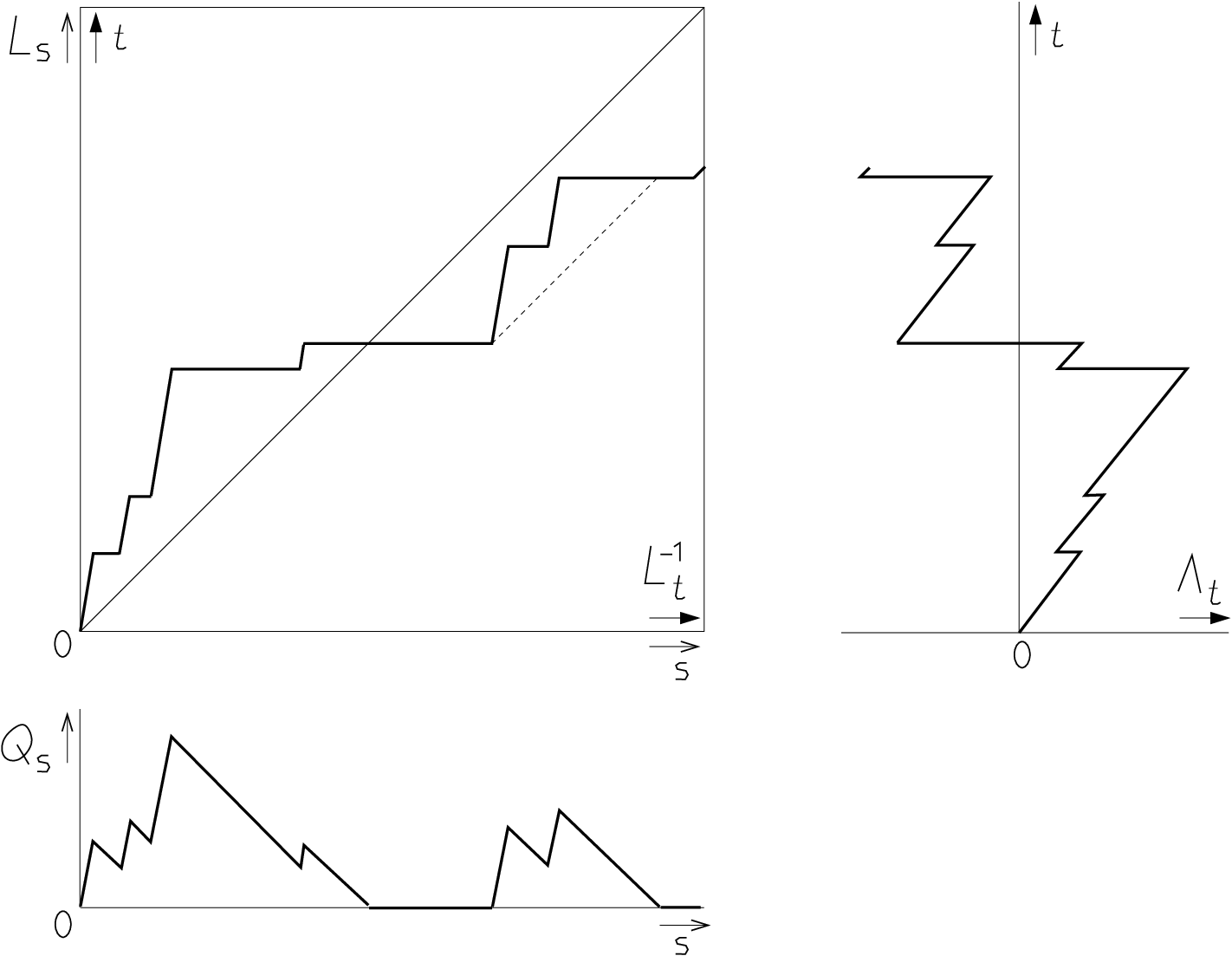
It can be intuitively seen, via a geometric argument involving the reflection of the space-time path of $\Lambda_{T}$ about the diagonal (see Figure 1), that the time taken for $\Lambda_{T}$ to first enter $(-\infty,0)$ is almost surely equal to the length of the excursion of $Q$ started at time $T$.

In this light, note also that $\Lambda_{T}$ cannot creep downwards because it is spectrally negative with paths of bounded variation (cf. Bertoin [2, Chap. VII]). Hence the overshoot at first passage of $\Lambda_{T}$ into $(-\infty,0)$ is almost surely strictly positive. It will turn out (Lemma 1.1) that this overshoot agrees with the idle period following the aforementioned excursion of $Q$.

The above analysis implies that, on finite intervals of time, $Q$ has finitely many excursions (busy periods) separated by positive-length idle periods. Denote by

the beginnings of the idle periods and by

their ends, see Figure 2. We choose the indexing so that $g(0)\leq 0<g(1)$. Let $N_{g}$ (respectively, $N_{d}$) be the point process with points $\{g(n):n\in\mathbb{Z}\}$ (respectively, $\{d(n):n\in\mathbb{Z}\}$). As $Q$ is a stationary process, $N_{g}$ and $N_{d}$ are jointly stationary with finite, nonzero, intensity [15] denoted by $\lambda$ (an expression for which is given by (26) and is derived in §4.3 below).

Corresponding to point processes $N_{g}$, $N_{d}$ we have the Palm probabilities $P_{g}$, $P_{d}$, respectively. Let us consider $Q$ under the measure $P_{d}$. Then $P_{d}(d(0)=0)=1$, i.e. the origin of time is placed at the beginning of a busy period. By the strong Markov property, the “cycles”

are i.i.d. under measure $P_{d}$. In particular, the pairs of random variables

are i.i.d. under $P_{d}$. Consider the triple

which is a function of $\mathsf{C}_{0}$. We are primarily interested in the $P_{d}$-law of $(B,I,Q^{*})$ Since, under $P_{d}$, the origin of time is placed at $d(0)$, we interpret $B,I,Q^{*}$ as the typical busy period, the typical idle period, and the maximum value of $Q$ over a typical busy period, respectively.

The next lemma is proved in [15]:

We now obtain an alternative expression for $B=g(1)-d(0)$ and $I=d(1)-g(1)$ in terms of the inverse local time.

Henceforth it will be convenient to work with the process $\Lambda=(\Lambda_{t},t\geq 0)$ where

Note also that $d(0)$ is an $(\mathcal{F}_{t})$-stopping time at which $X$ takes the value 0 and hence in our earlier notation $\Lambda_{t}=\Lambda_{d(0);t}$.

From the expression (6), and as discussed in the introduction of Section 2, we see that $B$ is simply the first time at which $\Lambda$ enters $(-\infty,0)$,

which is necessarily strictly positive thanks to the irregularity of $0$ for $(-\infty,0)$ for $\Lambda$. From (6) and (7) we see that

i.e. $I$ is, in absolute value, equal to the value of $\Lambda$ at the first time it becomes negative. Again we recall from the discussion at the beginning of Section 2 that $\Lambda$ cannot creep downwards and hence $I>0$ almost surely.

Consider now the random variable $Q^{*}=\sup_{d(0)<t<g(1)}Q_{t}$. If we define

we immediately see that

Recall that $P_{d}$ is the Palm probability with respect to the point process $\{d(n),n\in\mathbb{Z}\}$. The function

characterizes the joint law of the triple $(B,I,Q^{*})$ under $P_{d}$. Since $P_{d}(d(0)=0)=1$, we have that

Recalling the expressions (8), (9) and (11) for $B$, $I$ and $Q^{*}$, respectively, we write

Since our primary object is the process $\Lambda$ defined in (12), and in view of (4) and (13), it makes sense to consider the process on its canonical probability space and denote its law by $\mathbb{P}_{0}$. Then

The latter function may now be expressed in terms of so-called scale functions for spectrally negative Lévy processes. To define the latter, let

be the Laplace exponent of $\Lambda$ under $\mathbb{P}_{0}$. Then the, so-called, $q$-scale function for $(\Lambda,\mathbb{P}_{0})$, denoted by $W^{(q)}(x)$, satisfies $W^{(q)}(x)=0$ for $x<0$ and on $[0,\infty)$ it is the unique continuous (right continuous at the origin) monotone increasing function whose Laplace transform is given by

where

is the right inverse of $\psi_{\Lambda}$. (See for example the discussion in Chapter 9 of [17]).

In view of (8), (9), (11), and (13), we get the following corollary.

Clearly, formula (20) can be used to extract more detailed information about typical behaviour of $Q$. Let us first derive the distribution (Laplace transform) of the pair $(B,I)$ under the measure $P_{d}$. We have

To derive the limit, let us temporarily assume that $q=\alpha-\psi_{\Lambda}(\beta)>0$ and $\beta\geq 0$. Consider (16) in the form (18) and use the limiting result

from [17, Exercise 8.5] where the function $\Phi^{\beta}_{\Lambda}$ is the right inverse of $\psi_{\Lambda}^{\beta}$. That is to say

This gives

To remove the restriction that $\alpha>\psi_{\Lambda}(\beta)$ in (21) and replace it instead by just $\alpha\geq 0$, one may again proceed with an argument involving analytical extension taking care to note for the case that $\alpha=\psi_{\Lambda}(\beta)$,

We now show how the use of cycle formulae of Palm calculus enable us to find (Proposition 5.1 below) the joint law of the endpoints of an idle period conditional on the event that the idle period contains the origin of time. Also (Proposition 5.3 below) we characterise the joint law of the endpoints of a busy period, together with the maximum of $Q$ over this busy period, conditional on the event that the busy period contains the origin of time.

It is well-known that if $(\Omega,\mathcal{F},P)$ is endowed with a $P$-preserving flow $(\theta_{t},t\geq 0)$ (see end of Section 1) then for any random measure $M$ with finite intensity $\lambda_{M}$, and any point process $N$ with finite intensity $\lambda_{N}$ such that $M(B,\theta_{t}\omega)=M(B+t,\omega)$, $N(B,\theta_{t}\omega)=N(B+t,\omega)$, for $t\in\mathbb{R}$, $B$ Borel subset of $\mathbb{R}$, and $\omega\in\Omega$, and any nonnegative measurable $Z:\Omega\to\mathbb{R}$, we have

where $P_{M}$, $E_{M}$ (respectively, $P_{N}$, $E_{N}$) denotes Palm probability and expectation with respect to $M$ (respectively, $N$), $T_{0}$ is the first atom of $N$ which is $\leq 0$, and $T_{k},T_{k+1}$ are any two successive atoms of $N$.

The next result can be found for some special cases in [16] (diffusions), [15] (Lévy processes), and in [22] the general expression is derived. Here we offer a new proof in the general case based on (28).

References

- [1] Baccelli, F., and Brémaud, P. (2003) Elements of Queueing Theory: Palm Martingale Calculus and Stochastic Recurrences, 2nd edition, Springer.
- [2] Bertoin, J. (1996) Lévy processes. Cambridge University Press.
- [3] Bertoin, J. (1997) Exponential decay and ergodicity of completely asymmetric Lévy processes in a finite interval. Ann. Appl. Probab. 7, 56-169.
- [4] Bingham, N.H. (1975) Fluctuation theory in continuous time. Adv. Appl. Prob. 7, 705-766.
- [5] Blumenthal, R.M. and Getoor, R.K. (1968) Markov Processes and Potential Theory. Academic Press, New York.
- [6] Borodin, A.N., Salminen, P. (2002) Handbook of Brownian Motion - Facts and Formulae, 2nd ed. Birkhäuser.
- [7] Erdélyi, A., Magnus, W., Oberhettinger, F. and Tricomi, F.G. (1954) Tables of Integral Transforms. McGraw-Hill.
- [8] Fristedt, B.E. (1974) Sample functions of stochastic processes with stationary independent increments. Adv. Probab. 3, 241–396. Dekker, New York.
- [9] Hubalek, F. and Kyprianou A.E. (2010) Old and new examples of scale functions for spectrally negative Lévy processes. To appear in Sixth Seminar on Stochastic Analysis, Random Fields and Applications, eds R. Dalang, M. Dozzi, F. Russo. Progress in Probability, Birkhäuser.
- [10] Itô, K. and McKean, H.P. (1974) Diffusion Processes and Their Sample Paths. Springer Verlag.
- [11] Kallenberg, O. (1983) Random Measures. Academic Press.
- [12] Kallenberg, O. (2002) Foundations of Modern Probability. Springer-Verlag.
- [13] Konstantopoulos, T. and Last, G. (2000) On the dynamics and performance of stochastic fluid systems. J. Appl. Prob. 37, 652-667.
- [14] Konstantopoulos, T., Zazanis, M. and de Veciana, G. (1997) Conservation laws and reflection mappings with an application to multiclass mean value analysis for stochastic fluid queues. Stoch. Proc. Appl. 65, 139-146.
- [15] Konstantopoulos, T., Kyprianou, A. E. , Salminen, P. and Sirviö, M. (2008) Analysis of stochastic fluid queues driven by local time processes. Adv. Appl. Prob. 40(4), 1072-1103.
- [16] Kozlova, M. and Salminen, P. (2004) Diffusion local time storage. Stoch. Proc. Appl. 114, 211-229.
- [17] Kyprianou, A. E. (2006) Introductory Lectures on Fluctuations of Lévy Processes with Applications. Springer.
- [18] Kyprianou, A. E. and Palmowski, Z. (2004) A martingale review of some fluctuation theory for spectrally negative Lévy processes. Sem. Prob. 28, 16-29, Lecture Notes in Math., Springer.
- [19] Mannersalo, P., Norros, I. and Salminen, P. (2004) A storage process with local time input. Queueing Syst. 46, 557-577.
- [20] Pitman, J. (1986) Stationary excursions. Sem. Prob. XXI, 289-302, Lecture Notes in Math. 1247, Springer.
- [21] Salminen, P. (1993) On the distribution of diffusion local time. Stat. Prob. Letters 18, 219-225.
- [22] Sirviö, M. (2006) On an inverse subordinator storage. Helsinki University of Technology, Inst. Math. Report series A501.
- [23] Tsirelson, B. (2004) Non-classical stochastic flows and continuous products. Probability Surveys 1, 173-298.
- [24] Zolotarev, V.M. (1964) The first-passage time of a level and the behaviour at infinity for a class of processes with independent increments. Theory Prob. Appl. 9, 653-664.