Strategies for improving the efficiency of quantum Monte Carlo calculations
Abstract
We describe a number of strategies for minimizing and calculating accurately the statistical uncertainty in quantum Monte Carlo calculations. We investigate the impact of the sampling algorithm on the efficiency of the variational Monte Carlo method. Our finding that a relative time-step ratio of is optimal in DMC is in agreement with the result of [J. Vrbik and S. M. Rothstein, Intern. J. Quantum Chem. 29, 461-468 (1986)]. Finally, we discuss the removal of serial correlation from data sets by reblocking, setting out criteria for the choice of block length and quantifying the effects of the uncertainty in the estimated correlation length.
pacs
02.70.Ss, 31.15.A-, 71.15.-mI Introduction
Quantum Monte Carlo (QMC) methods are a class of stochastic ab initio techniques for solving the many-body Schrödinger equation [1, 2]. They are capable of achieving accuracy comparable to that of post-Hartree-Fock quantum-chemistry techniques but with a much lower computational cost. The diffusion Monte Carlo (DMC) method in particular has no close competitors for calculations of the energy of bulk periodic systems.
The utility of QMC stems from the fact that the cost of achieving a given error bar scales as for typical systems 11 1 Ultimately, for large the scaling of DMC with system size becomes exponential as discussed in N. Nemec, Phys. Rev. B 81, 035119 (2010)., where is the number of quantum particles. The method is most useful when studying systems for which quantum-chemistry calculations are infeasible and density functional theory does not give a sufficiently accurate description of electronic correlation. The algorithms are intrinsically parallel, allowing QMC to take full advantage of developments in computer technology. The variational Monte Carlo (VMC) algorithm, for example, is almost perfectly parallelizable. Furthermore, existing QMC implementations are easily extended to different systems. One may apply the same basic algorithms, changing only the form of the trial wave function and the Hamiltonian, to systems comprising any combination of particles and interparticle interactions. Because the trial wave function can be an explicit function of interparticle distances, the Kato cusp conditions and other correlation effects can be described compactly, without the need for large expansions of many determinants and other unwieldy functional forms [3]. For a comprehensive overview of VMC and DMC, the reader is directed to Refs. 2, 1, 4, 5.
The practical challenges facing QMC are largely concerned with improving the efficiency of the algorithms and the design of new trial wave functions. The computational expense of a large calculation necessitates careful selection of the operational parameters. Typically one has a certain amount of computer time available within which one wishes to achieve the smallest possible statistical error in the final result. In addition, the extraction of an accurate statistical error bar from serially correlated data is itself nontrivial. In this paper, we outline how to choose the optimal parameters and algorithms at the different stages of a QMC calculation and describe how to process the resulting data.
This paper is structured as follows. Section II gives an analysis of the many related factors contributing to the efficiency of VMC calculations. Section III describes how to improve the efficiency of DMC time step extrapolation. In Sec. IV we discuss the calculation of accurate error bars using the reblocking method and describe a robust scheme for choosing block lengths. We demonstrate in Sec. V that uncertainty in the estimated correlation length results in an error in the statistical error bar that can significantly enhance the probability of observing outliers. Finally, we draw our conclusions in Sec. VI. We use Hartree atomic units () throughout this article.
II Efficiency of VMC calculations
II.1 Method
In this section, we discuss practical schemes for achieving maximal efficiency within the VMC method. We focus on three aspects of a VMC calculation. The first is the sampling algorithm, which is how moves are proposed. The second is the use of decorrelation loops, which consist of additional moves for which we avoid evaluating the local energy. We will demonstrate that decorrelation loops can offer a twofold increase in efficiency. To our knowledge, there are no quantitative investigations of decorrelation loops in the literature. The third factor we consider is the choice of time step, which governs the width of the transition probability density function (PDF). Our findings are summarized by the set of recommendations in Sec. II.5.
Variational Monte Carlo is the simplest and least computationally expensive QMC method. In the VMC method, the expectation value of the Hamiltonian with respect to a trial wave function is calculated using a stochastic integration technique, giving a variational estimate for the ground state energy,
| (1) |
where is the local energy and is a vector describing all the particle positions. The set contains energies and is produced by evaluating at points in configuration space distributed according to .
Due to the finite number of samples , the VMC estimate of the energy of Eq. (1) has a statistical error , where is the standard deviation of the local-energy distribution and is the correlation length [6] of the sequence of local energies.
The quantity only depends on the system and the trial wave function, whereas also depends on the sampling algorithm. Thus, for a given system, trial wave function, and sampling algorithm, the statistical error diminishes with the number of configurations sampled as . Suppose one VMC step takes a time . A VMC calculation is more efficient the less time it requires to reach a given statistical error , so if a VMC run takes a CPU time of to sample configurations, an appropriate measure of its efficiency is
| (2) |
which is independent of . The efficiency of a VMC calculation can be improved by reducing the product .
II.2 VMC sampling
The electronic configurations are generated using the Metropolis algorithm [7], where a move from to is proposed with probability , and is accepted (i.e., ) with probability
| (3) |
or otherwise rejected (i.e., ). In fact, if the wave function can be factorized, one can greatly improve efficiency using multi-level sampling [8]. All of our calculations use two-level sampling, in which we accept or reject the move first based on the Slater determinant part of and then (if the Slater part of the move was accepted) based on the Jastrow factor [1].
A simple, commonly used choice for is the product of Gaussian distributions of variance (standard deviation ) for each of the Cartesian components of the displacement of each electron. By analogy with DMC, is often referred to as the VMC “time step,” although there is no notion of time in the VMC formalism. We shall restrict our analysis to the case of Gaussian transition probabilities. Alternatives to this choice have been proposed [9, 10], but these studies focus on the statistical improvement for a given number of iterations, and do not analyze the total efficiency. The simplicity of the Gaussian distribution represents an efficiency advantage that is hard to offset with more exotic distributions. Nonetheless, the conclusions presented here should mostly be applicable to other transition probabilities.
II.2.1 Configuration-by-configuration and electron-by-electron sampling
In the sampling algorithm we have just described, to go from to we propose an entire configuration move, and we accept it or reject it with a single decision. This is what we call configuration-by-configuration sampling (CBCS).
However, it is possible to generate from by proposing successive single-electron moves and accepting or rejecting each of them individually. The resulting algorithm is electron-by-electron sampling (EBES), which allows larger moves to be accepted, greatly reducing . This comes at the cost of an increase in , because evaluating the acceptance probabilities in EBES takes longer than computing the single acceptance probability in CBCS.
II.2.2 Averaging local energies over proposed moves
It is possible to replace the average in Eq. (1) with an expression where the local energies at and are multiplied by the acceptance and rejection probabilities, respectively, and summed together. For CBCS, the expression is [11]:
| (4) | |||||
This expression is also a valid approximation to the VMC energy, with the advantage that rejected moves contribute to the sum, adding new data and improving the statistics, especially when the acceptance ratio is low. This translates into a reduction in . The evaluation of the additional local energies increases , however. We investigate the balance of these factors below for CBCS.
We have avoided averaging the energy over proposed moves in EBES since even with refinements it has been found to be less efficient than the unmodified algorithm [12].
II.2.3 Decorrelation loops
It is possible to go from to by proposing configuration moves in turn instead of just one. In this scheme one generates a sample of local energies by performing a calculation consisting of moves and evaluating the local energy at every th configuration.
The cost of one step of a VMC calculation with a decorrelation loop of length is
| (5) |
where is the time it takes to propose and accept or reject a single configuration move and is the time it takes to evaluate the local energy 22 2 The details of the implementation may need to be taken into account in this expression. An implementation could detect whether all moves have been rejected between evaluations of the local energy to avoid unnecessary re-evaluations. In this case, the probability of not having to calculate a local energy is the probability of having rejected consecutive moves, and becomes ..
It is possible to establish the precise form of the correlation length as a function of . When , is
| (6) |
where is the autocorrelation of local energies separated by steps,
| (7) |
If we assume that the autocorrelation is dominated by a single exponential term, i.e., then Eq. (6) becomes
| (8) |
Hence , and the correlation length at is
| (9) | |||||
which falls off as if is large. From Eqs. (2), (5), and (9) we can build the full expression for , and it is possible to find the value of that maximizes analytically from estimates of , , and .
The usefulness of decorrelation loops depends on how costly it is to evaluate local energies and how much serial correlation is present. Were it the case that local energies took no time to evaluate (i.e., ), the inclusion of decorrelation loops would not increase the efficiency , and if no serial correlation were present then , and increasing would simply increase the cost of each step.
II.3 Automatic optimization of
Although the VMC algorithm is valid for any positive time step, the efficiency of the method depends strongly on . An appropriate time step for EBES VMC can be very roughly estimated as being such that the root-mean-square (RMS) distance moved by each electron at each time step is equal to the most important physical length scale in the problem. Assuming the acceptance probability of electron moves is approximately 50%, the RMS distance diffused is in three dimensions. In an electron gas the only physical length scale is the radius of the sphere that contains one electron on average, so the required time step is . In an atom the length scale is somewhere between the Bohr radius , where is the atomic number, and 1 a.u. However, it is clear that these crude choices are far from optimal.
There are two commonly-used approximate methods for choosing ; aiming to achieve an acceptance ratio of 50% (the 50% rule), and maximizing the diffusion constant. Both can be implemented so that this optimization occurs automatically and inexpensively at the beginning of a VMC run.
In the “50% rule” it is assumed that the ratio of accepted moves to proposed moves is representative of the sampling efficiency, and that a value of 50% is near-optimal. In general, the two limits of 0% and 100% acceptance correspond to a failure to properly explore phase space, but there is no particular reason why should correspond to optimal sampling.
The diffusion constant can be computed as the average of the squared displacement between consecutive configurations and 33 3 When we use decorrelation loops, we define as the average of the squared displacement between consecutive configurations within the decorrelation loop, not between those for which the energy is evaluated.. One might reasonably assume that choosing to maximize is an efficient strategy, although maximization of does not necessarily correspond to optimal sampling. For example, in a CBCS study of the homogeneous electron gas, rigidly translating all of the electrons together results in a very large diffusion constant but clearly corresponds to poor exploration of phase space.
II.4 Empirical data and analysis
We shall consider four basic choices to be made when performing a VMC calculation with a Gaussian transition-probability density: whether to use CBCS or EBES, whether to average local energies over proposed moves, the value of the “time step” , and the length of the decorrelation loop .
In order to study the effect of these choices, we have performed VMC calculations for a set of six representative systems: a pseudopotential N atom, an all-electron O atom, a pseudopotential NiO molecule, an all-electron N2H4 molecule, a three-dimensional homogeneous electron gas (HEG) composed of 38 electrons at a density parameter of a.u., and a 16-atom supercell of a pseudopotential C diamond crystal 44 4 Our calculations were performed on a cluster of eight 24GB, dual-socket, quad-core, 2.66GHz Intel Core i7 processors. However, we have only quoted ratios of efficiencies in this paper, which should be largely architecture-independent.. For each system, we tested two trial wave functions: one of Slater-Jastrow form [1, 13] and another of Slater-Jastrow-backflow form [14, 15].
| System | ||||||||||
|---|---|---|---|---|---|---|---|---|---|---|
| N (pp) | 0. | 20 | 3 | 55% | 1. | 00 | 0. | 52 | 0. | 65 |
| O | 0. | 05 | 3 | 58% | 0. | 94 | 0. | 40 | 0. | 68 |
| NiO (pp) | 0. | 20 | 5 | 44% | 0. | 94 | 0. | 39 | 0. | 41 |
| N2H4 | 0. | 05 | 3 | 64% | 0. | 62 | 0. | 09 | 0. | 71 |
| HEG | 1. | 00 | 3 | 37% | 0. | 93 | 0. | 96 | 0. | 73 |
| Diamond | 1. | 00 | 3 | 32% | 0. | 94 | 0. | 66 | 0. | 60 |
| System | ||||||||||
|---|---|---|---|---|---|---|---|---|---|---|
| N (pp) | 0. | 10 | 8 | 32% | 0. | 87 | 0. | 90 | 0. | 33 |
| O | 0. | 01 | 8 | 27% | 0. | 82 | 0. | 82 | 0. | 64 |
| NiO (pp) | 0. | 02 | 36 | 17% | 0. | 70 | 1. | 00 | 0. | 13 |
| N2H4 | 0. | 01 | 13 | 16% | 0. | 59 | 1. | 00 | 0. | 42 |
| HEG | 0. | 05 | 36 | 9% | 0. | 54 | 0. | 88 | 0. | 47 |
| Diamond | 0. | 02 | 36 | 11% | 0. | 25 | 0. | 79 | 0. | 13 |
For each system and wave function, we have performed calculations using EBES and CBCS, and for CBCS we have run calculations with and without averaging over proposed moves. Finally, for each system, wave function, and sampling method, we have performed 160 VMC calculations covering 16 different values of and 10 different values of . In each case we have identified the maximum efficiency . To assess the performance of the “50% rule,” we have located the value of the time step whose acceptance ratio is closest to and compared the efficiency with . To assess the performance of maximizing the diffusion constant, we have located the value of the time step with the maximum and compared the efficiency with . To assess the importance of decorrelation loops, we have compared the efficiency with . The results of these comparisons are given in Table 1 for EBES and Table 2 for CBCS, in both cases for the Slater-Jastrow wave function only; the data for the Slater-Jastrow-backflow wave function are nearly identical and are not shown.
For the periodic systems the acceptance ratio in EBES does not reach zero as is increased, and as a consequence the efficiency presents a plateau in that region, where we find that is close to . In EBES we also find that the “50% rule” consistently gives efficiencies within 10% of the maximum, with the exception of the N2H4 molecule, where the optimal acceptance ratio is larger. Maximization of the diffusion constant in EBES consistently gives time steps that are too large and yields efficiencies below about 50% of the maximum possible for finite systems, and between 65% and 95% of the maximum for periodic systems. In CBCS, maximizing the diffusion constant achieves reasonable efficiencies, often within 10% of the maximum value, while the “50% rule” gives increasingly poor results as the system size increases. Decorrelation loops improve the efficiency in EBES by between 50% and 150%. In CBCS these become more important and enhance by up to a factor of seven.
| System | SJ | SJB | SJ | SJB | ||||||
|---|---|---|---|---|---|---|---|---|---|---|
| N (pp) | 5 | 1. | 05 | 0. | 90 | 1. | 22 | 1. | 24 | |
| O | 8 | 1. | 47 | 1. | 07 | 1. | 10 | 1. | 17 | |
| NiO (pp) | 16 | 1. | 65 | 1. | 22 | 1. | 38 | 1. | 52 | |
| N2H4 | 18 | 1. | 93 | 0. | 83 | 1. | 11 | 1. | 53 | |
| HEG | 38 | 3. | 11 | 1. | 95 | 1. | 27 | 1. | 25 | |
| Diamond | 64 | 4. | 70 | 2. | 36 | 1. | 14 | 1. | 24 | |
In Table 3 we compare the maximum efficiency encountered in EBES with that in CBCS for Slater-Jastrow (SJ) and Slater-Jastrow-backflow (SJB) wave functions. The fifth and sixth columns of Table 3 show the comparison for CBCS when a single energy is evaluated per configuration move (), and where averages of local energies over proposed moves are carried out ().
EBES is more efficient in all cases, with the exception of the backflow calculations on the pseudopotential N atom and the all-electron N2H4 molecule. The improvement in efficiency that EBES offers over CBCS increases with system size. Averaging energies over proposed moves is found to be less efficient in every case.
II.5 Recommendations
Our key finding is that decorrelation loops increase the efficiency of EBES by roughly a factor of two and that of CBCS by much more. One can use the expressions in Sec. II.2.3 to determine the optimal loop length , although in practice a decorrelation period of delivers near-optimal efficiency in the EBES algorithm for a wide range of systems.
Based on the data presented in Sec. II.4, we suggest that EBES should nearly always be used in VMC, the only possible exception being for small systems with fewer than about 20 electrons when backflow is used. (Even in this case, CBCS is not much more efficient than EBES.) When using EBES, one should use the “50% rule” to optimize the time step . If CBCS is used, one should maximize the diffusion constant to optimize the time step . Finally, we find that accumulation methods which average local energies over proposed moves are less efficient for every system tested.
III Optimizing DMC time-step extrapolation
DMC is a Green’s function projector method for solving the Schrödinger equation in imaginary time. In DMC, the ground state distribution is represented by the density of walkers (points in configuration space) rather than by an analytic function. Propagation of a population of walkers in imaginary time projects out the ground-state component of the initial DMC wave function [16, 1].
The DMC algorithm is only accurate in the limit of small time step . However, the computational effort required to achieve a given error bar goes as , ruling out the use of infinitesimal time steps in practice. Hence, where high accuracy is required, two or more finite time steps are generally used and the ground-state energy is obtained by extrapolating to [1, 2]. Here we explain how the statistical error in a zero-time-step extrapolate may be minimized by a judicious choice of time steps , and the prudent deployment of a limited total computing time between those time steps. Note: since our paper was published, it has been drawn to our attention that the principal result obtained in this section was previously derived in Ref. 17.
For sufficiently small , the DMC energy scales linearly with the time step as . Suppose we calculate at different time steps in the linear-bias regime, where each has an associated statistical uncertainty . The error bars fall off with the time step and the CPU time devoted to the calculation as , where is a constant. To determine the ground-state energy at zero time step , we minimize the error of the linear fit,
| (10) | |||||
with respect to and . Setting , we obtain
| (11) |
Assuming the data are Gaussian-distributed, the square of the standard error in the extrapolate is
As expected the standard error falls off as the time steps are increased and as more time is dedicated to the calculations. However, should not be increased beyond , the limit of the region in which the bias is linear. The effort allocated to the calculations cannot be increased indefinitely because one is constrained by the total time for all of the simulations. We now minimize subject to the constraint that is fixed.
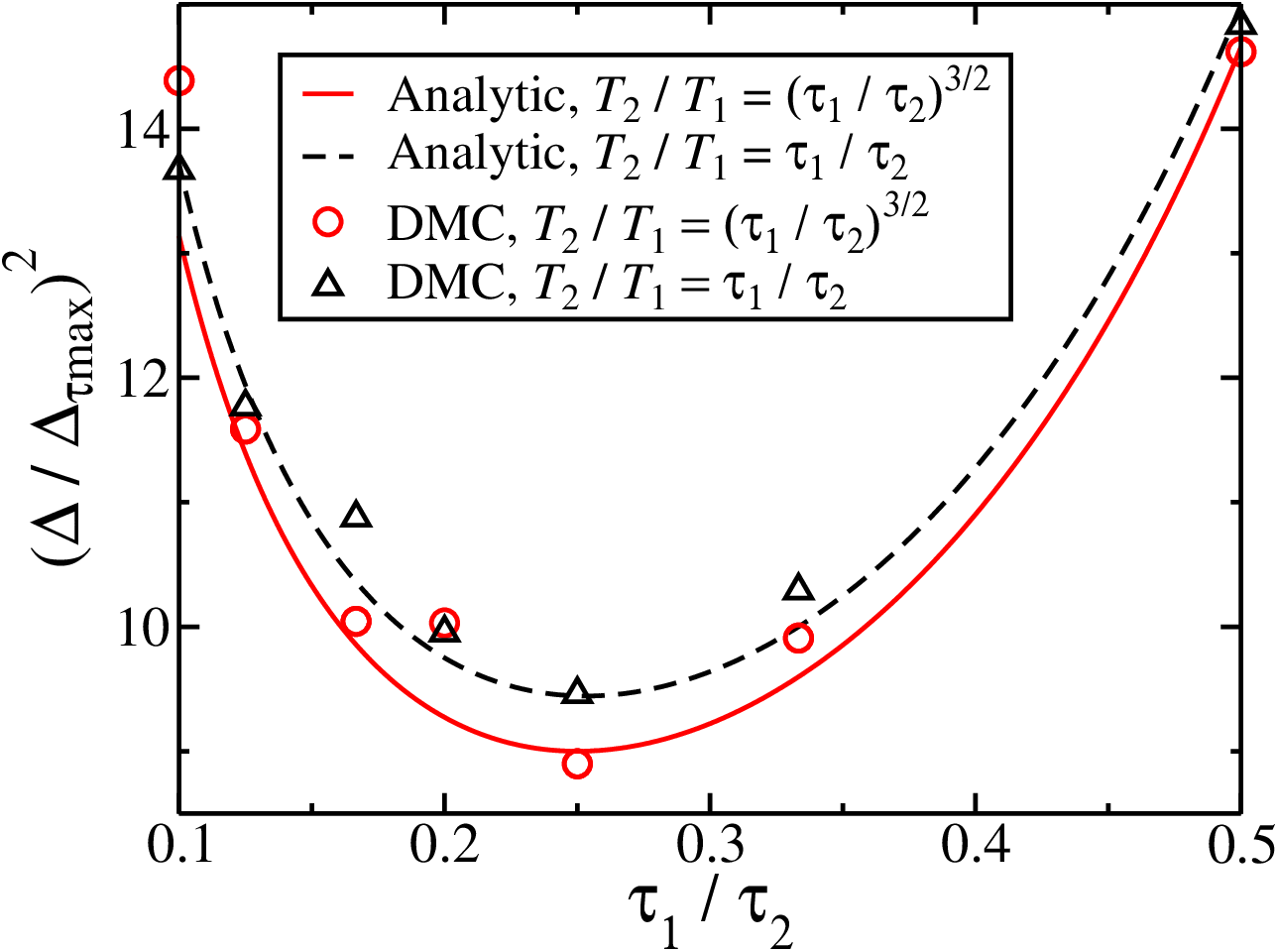
Let us first suppose that we are to perform just simulations. We start by fixing the time steps and , and minimizing with respect to the run lengths in the presence of a Lagrange multiplier to constrain the total run time . This yields the optimal simulation durations and . This deployment attempts to reduce the error bar on the calculation with the smallest time step beyond the distribution of effort that would ensure error bars of equal size. Without loss of generality, we now assume that , with pinned near the boundary of the linear regime, and we search for the optimal time step . Using the optimal durations and , minimization of reveals that the optimal choice of time step is . The corresponding optimal physical run times are therefore and . The full dependence of the final error upon the relative time step is shown in Fig. 1.
Now suppose that more than two time steps are used to perform the extrapolation. We find that is minimized when all the computational effort is dedicated to the two points that are nearest to having a relative time step of and have the largest maximum value of . Computational effort should therefore be focused solely on that optimal pair as long as the linear regime is well-defined. There is thus no advantage to using more than data points.
Our scheme is the optimal extrapolation procedure when the extent of the linear regime is known. The strategy is thus highly applicable to studies of many similar systems where the linear regime can be assumed to be the same for multiple runs. For systems where the behavior of the time step bias has not been established, one has no alternative but to perform multiple runs over a wide domain of time steps and determine where the spectrum first increases superlinearly. In such cases, one can use the RMS distance diffused by an electron over a single step as an initial order-of-magnitude estimate for where the linear regime begins. For all-electron atomic systems, for example, one would expect the linear regime to occur for time steps less than of the order , where is the largest atomic number occurring in the system. This choice of time step ensures that the RMS distance diffused is equal to one Bohr radius of the largest atom under study. For a homogeneous electron gas, where the only physically-significant length scale is defined by the density, the equivalent time step would be , where is the radius of the sphere (circle in 2D) that contains one electron on average, and is the dimensionality. Time step bias is reduced when the modifications of Ref. 5 are made to the DMC Green’s function, and also when higher-quality wave functions are used.
If one has accumulated a significant set of results for in determining the extent of the linear regime, the prescription for minimizing the error in the extrapolate has the potential to differ from the two-run procedure. If one has a large amount of computing time remaining after determining , the two-run approach is unchanged. In the event that little computing time remains after determining , one should devote the remaining time to the run whose contribution falls the quickest with computer time, i.e., the run with the most negative value of , which may be found from Eq. (III).
Avoiding higher order fitting functions and using only data from within the linear regime for the extrapolation is the most robust strategy. Though the formalism here can be extended to study higher-order fitting functions, finding the appropriate regimes for higher-order terms would require a larger amount of computational effort and there is a danger of numerical stability and branching problems affecting calculations for very large . Linear extrapolation is always an option since the leading-order term in the bias is known to be .
We highlight the benefits of the two-run extrapolation procedure with an example calculation on the 1D HEG. Once the maximum allowed time step in the linear regime had been determined, pairs of runs were performed at and incrementally smaller time steps . The pairs of runs were each performed using the same total amount of computing time. The time was distributed either to ensure equal-sized error bars or according to the prescription to guarantee minimal final extrapolated error. The simulation times were sufficient to ensure that the data could be reblocked for accurate error estimates. The final extrapolated energy estimates all agreed to within the expected uncertainty, consistent with the assertion that all of the time steps are within the linear regime. The results shown in Fig. 1 highlight that, for the range of tested, there is strong agreement between the analytical prediction and the DMC results. In particular, the error bar on the extrapolate with the optimal distribution of effort is clearly minimized by the choice . The distribution of effort according to yields a modest computational advantage over the choice .
In summary, to minimize the statistical error bar on the DMC energy extrapolated to zero time step, one should perform one DMC calculation at the largest time step for which the bias is still linear in the time step and a second DMC calculation with time step . Eight times as much computational effort should be devoted to the latter calculation as to the former. One could use a similar approach to optimize the efficiency of extrapolating to infinite population or to infinite system size in a QMC study of condensed-matter systems.
IV Reblocking
The use of small time steps in DMC results in serially-correlated data. For accurate estimates of the statistical uncertainties of DMC expectation values, the serial correlation must be accounted for. Here, we investigate reblocking [18], which is advantageous due to its computational convenience and ease of implementation. We propose a scheme for the choice of block length such that accurate error bars may be reliably determined when an estimate for the correlation length is unavailable and must be obtained directly from the data.
For most random processes used in Monte Carlo methods the serial correlation is purely positive, so that the standard error (treating all samples as independent) should be multiplied by an error factor . Let the new estimate of the standard error be , and let be divided by the estimated correlation length, i.e., measures the estimated effective number of steps. We may express as
| (13) |
where is the sample variance of the data points and the error factor is the square root of the estimated correlation length [6]. As each step of a QMC calculation is associated with a time step measured in physical units, a correlation time in physical units can be defined as . In the limit , the integrated correlation time becomes independent of and takes a value characteristic of the system under study.
To estimate from a set of data points , there are several commonly-used approaches: computing the correlation length, reblocking, or using resampling techniques like the jackknife and bootstrap methods [6, 18, 19, 20]. Here we have focused on the reblocking method because it is computationally convenient (and conceptually very simple) to apply reblocking continuously as local observable data are appended to the stored results, vastly reducing memory requirements [21]. A naive calculation of the correlation-corrected statistical error necessitates the storage of observable values, whereas reblocking on-the-fly reduces this to .
Reblocking is a method in which a sequence of serially correlated data points is divided into contiguous blocks of length , and the raw data are averaged within each of these blocks, defining a new data set of length . The naive variance of the reblocked estimate of the mean is larger than that of the original data, although the mean itself is unchanged. The estimated error initially increases with , reaching a plateau once the serial correlation has approximately been removed from the data. When approaches , the plot becomes very noisy due to the small number of blocks.
The reblocking analysis of a typical DMC run is shown in Fig. 2. The fundamental difficulty in interpreting this kind of data is the choice of an appropriate block size. In the case presented here, the run time of 900000 time steps was sufficiently long to form a clear plateau in the reblock plot. However, individually inspecting the reblocked data of each calculation to make a choice by eye is neither objective nor efficient. Table 4 shows the estimated correlation lengths from reblocking the Li data with different block lengths.
| Estimated | |
|---|---|
| 1 | 1.762(4) |
| 2 | 3.140(9) |
| 3 | 5.51(2) |
| 4 | 9.34(5) |
| 5 | 14.7(1) |
| 6 | 21.0(2) |
| 7 | 28.9(5) |
| 8 | 34.0(8) |
| 9 | 36(1) |
| 10 | 39(2) |
| 11 | 40(3) |
| 12 | 37(3) |
| 13 | 42(6) |
| 14 | 44(8) |
A simple yet robust algorithm for automatically choosing the best block size is as follows. Following Ref. 6, the block size
| (14) |
offers an appropriate balance between the systematic and the statistical error in the estimate of the standard error for any set of data points with the integrated correlation length . If a good estimate for is available before the data are analyzed, it is best to use this and thereby make the choice of the block size independent of the statistical data themselves. In many studies, several runs on similar systems are needed or the knowledge of can be used to extrapolate to small time steps. In such cases it is best to estimate once and reuse it for the choice of in subsequent calculations, provided that the physical system and wave-function quality (and thus the correlation length) are unchanged. The error factor obtained in each case can then be used to double-check the transferability of the estimated correlation length without influencing the choice of , so that there is no bias from manually making a data-dependent choice.
If an independent estimate for is not available, it has to be obtained from the analyzed data themselves. In this case, the estimated correlation length depends on the choice of , so the condition for becomes recursive. We consider block sizes that are powers of and start with the largest block size possible, decreasing and examining the error factor. The optimal block size is then the last value of for which the inequality is satisfied. We may restrict to powers of since the block length is expected to be logarithmically distributed.
In a reblocking analysis for data points, the relative error in the error factor for a given block size depends only on the number of blocks as
| (15) |
Assuming that a user would typically expect at least one significant digit in the standard error, we can further define a straightforward criterion for the success of a reblocking analysis: if , the analysis can be accepted as successful, otherwise the reliability of the result is questionable and one should gather more data. Except for systems with distinct correlation times at extremely different scales, this criterion is expected to be reliable in all typical cases occurring in QMC. More than one correlation time might occur in weakly bound molecules; the longest correlation time is defined by the size of the molecule and the shortest is determined by the Bohr radius of the nucleus with the highest atomic number. In such cases, it may be necessary to accumulate more data; the block size should clearly be determined by the longest correlation length.
In summary, when using reblocking to remove serial correlation from QMC data, one should ideally obtain an accurate estimate of the correlation length separate from the data being analyzed and use to determine the block length [6]. If this is not possible, one should aim to satisfy the inequalities and for a reliable and accurate estimate of the error.
All methods of accurately calculating the error bar from serially-correlated data implicitly estimate the correlation length. The noise and associated uncertainty in estimates of the correlation length introduce error into the estimated statistical error bar. In the next section we describe how this can increase the apparent number of outlying results.
V Outliers in QMC results
V.1 Introduction
In this section, we investigate the frequency with which “outliers” occur in QMC results. We define an outlier as a result located more than a given number of estimated error bars from the underlying mean value. For example, one may fit a straight line to DMC energies at small . If there are sufficient data points, the linear fit is a good estimate of the underlying mean; one would usually expect, by the central limit theorem (CLT), a fraction of the points to deviate from the fitted function by more than a single error bar. Here we address the observation that QMC estimates can lie outside statistical error bars of the underlying mean more often than one would expect were the error bars correctly describing the width of an underlying Gaussian distribution. We will demonstrate that uncertainty in the estimated correlation length is largely responsible for this effect.
We begin with direct observation of the numbers of outliers for two systems, the C atom and the Si crystal. By performing a large number of short VMC calculations for each system, we count directly the number of energies occurring more than error bars from the underlying mean, where the error is estimated separately for each run. Each estimate of the statistical error is also implicitly an estimate of the correlation length, as described by Eq. (13).
To complement the direct approach, we then derive an analytic expression for the fraction of points expected to lie more than error bars from the mean under the assumption that the distribution of local energies is Gaussian. The resulting expression depends on the distribution of estimated correlation lengths. Finally, we compare the expected result from this purely Gaussian model process with that found earlier from VMC, forming conclusions about the validity of the Gaussian assumption and the origin of outliers.
V.2 VMC calculations
We have performed a large number of VMC calculations for two typical systems; the all-electron carbon atom and a periodic crystalline silicon system. For the C atom we performed , , and calculations of length , , and steps, respectively. The Si system used a periodic simulation cell containing 54 silicon atoms, where the electrons are described by pseudopotentials. For the Si system, we performed , , and calculations of length , , and steps, respectively.
A short calculation yields an energy and estimated error. From the data we estimate the probability of observing a VMC energy at a position more than from the true mean , where and is the estimated error bar, itself also a random variable. The underlying mean is calculated accurately using a much longer run. If the error bars exactly described the width of an underlying Gaussian distribution, one would expect . The symbols in Figs. 4 and 5 show the deviation of the VMC results from this ideal case.
By estimating the statistical error bar for each run, we are able to estimate , which is the distribution of the estimated effective number of steps , where is the number of VMC steps and is the error factor of Eq. (13). An example kernel estimate of is shown in Fig. 3; one can see that is occasionally larger than . This is clearly unphysical, stemming from noise in the estimate of the correlation length, and results in underestimation of the statistical error bar. The distribution appears to decay at large as , where is between and .
V.3 Gaussian model
We now attempt to replace VMC sampling with an ideal process where the underlying distributions are Gaussian. Our starting point is the distribution of local energies, , from which energies are drawn at successive points along the random walk in configuration space. The quantity of interest is again the probability of observing a sample mean energy at a position more than from the true mean .
Let us assume that the distribution of local energies is Gaussian,
| (16) |
where is the variance of the distribution. Consider drawing samples from the PDF of Eq. (16) using the Metropolis algorithm; this yields independent samples due to serial correlation. For this simple case the sample mean, , has the distribution
| (17) |
The statistical error bar on is calculated from the same set of local energies as the estimate itself. However, since estimates of the correlation length are subject to noise, there is uncertainty in the effective number of independent samples. Although this leaves unaffected, it does influence the estimated error. As before, we define as the random estimate of and again refer to the PDF from which is drawn.
It is well-known that a sum of squares of normally-distributed random numbers follows the chi-square distribution [22]. Since the error bar is related to the sample variance through Eq. (13), we can write down the bivariate PDF for and ,
| (18) |
where is only allowed to take positive values and is the Gamma function. It is straightforward to find analytically the probability of observing an energy more than error bars from the mean as a function of and . This is done by integrating Eq. (17),
| (19) |
To find the desired probability, , we evaluate the expectation value of Eq. (19) with respect to the distribution of and ,
| (20) | |||||
where we have used the fact that the sample mean and sample variance are independent for Gaussian distributed random variables [23, 24]. To evaluate the integral of Eq. (20), we require the distribution and an accurate estimate of the true effective number of steps, . We will take these quantities from the VMC results of Sec. V.2, so that the integral of Eq. (20) represents an ideal Gaussian process accompanied by the uncertainty in the number of independent samples (and thus the correlation length) that we observe in VMC. The integral of Eq. (20) can then be evaluated numerically.
V.4 Results


Figures 4 and 5 show the actual fractions of outliers from the VMC calculations compared with those predicted by Eq. (20), which used and from the VMC calculations but otherwise assumed a model Gaussian process. The fraction of points occurring more than error bars from the mean has been offset by in the figures to highlight the deviation from the result when the correlation length is known exactly, i.e., .
When takes smaller values, the uncertainty in the correlation length is greater and the fraction of points which may be classified as outliers is larger. A poor trial wave function could also contribute to the effect by reducing the sampling efficiency. In the case of the C atom, instead of the probability of observing an energy more than error bars from the mean that one would expect on the basis of Gaussian statistics, the VMC results are consistent with a probability (for runs of local energies). For the C and Si systems, estimating the error bars for each short run using a single more accurate estimate of the correlation length (from a single longer run or by averaging the estimates from each shorter run), results in a return to .
For systems exhibiting singularities in the local energy, the CLT converges only very slowly and one might expect the non-Gaussian character of to play a role in determining the frequency with which outliers are observed [25]. Singularities in the local energy arise when the description of the wave-function nodes is inexact, as is the case for the C and Si systems considered here, and when the cusp conditions are unfulfilled.
We find that the contribution from the non-Gaussian parts of the energy PDF towards the frequency of outliers is statistically insignificant. The evidence for this is twofold; first, the integrals based on a purely Gaussian agree very well with the VMC data, suggesting that uncertainty in the correlation length is almost solely responsible for the effect. Secondly, attempting to fit a function with power law tails (of the form suggested in Ref. 25) to the VMC energies yields very small values for the weight under the tails (usually within error bars of zero), even though the distribution of local energies is itself manifestly non-Gaussian 55 5 We form a biased estimate for the weight of the power-law tails by fitting Eq. (48) of Ref. 25 to the distribution of energies obtained from VMC runs, each of steps. We find and for the C atom and the bulk Si system, respectively. The error in the fit was per data point for the C atom and per data point for the bulk Si system.
In conclusion, when there is too little data to make an accurate estimate of the correlation length, the estimated error is subject to an uncertainty that increases the probability of observing outliers. For isolated calculations of a single run, the problem amounts to the gathering of sufficient data for an accurate estimate of the correlation length. Where dependence upon several parameters is being investigated for large systems, one should calculate accurately the correlation length from a single long run or by averaging many estimates from shorter runs. The accurate estimate of the correlation length can then be interpreted as the square of the error factor, , and used to calculate the error bars on related calculations in two ways: either by guiding the choice of block length () or by multiplying the unreblocked error by ; the two estimates should be roughly consistent.
VI Conclusions
In this paper we have developed and carefully tested new ways of improving the efficiency of QMC calculations.
Our analysis of VMC efficiency shows that the use of decorrelation loops approximately doubles the efficiency of EBES, with a loop of three moves providing the greatest benefit for a wide range of systems. The improvement in efficiency for CBCS is much greater. However, we find that EBES rather than CBCS yields a higher efficiency, except in small systems where backflow transformations are used. Of the automatic schemes for optimizing the time step that we have considered, attempting to achieve a move acceptance ratio of leads to the greatest efficiency within EBES.
For the extrapolation of DMC energies to zero time step there is a clear optimal strategy. One must first find the largest time step for which the energy can be considered to vary linearly with time step. One should then minimize the error in the extrapolate by performing calculations at two different time steps; the first at with computational effort , and the second at with computational effort , where is the total computing time available.
The reblocking method of removing serial correlation from QMC data offers a significant computational advantage over other methods. Ideally, when choosing a block size, one should estimate the correlation length for a system independently of the serially-correlated data themselves. The optimal block length should be chosen such that and [where is the number of data points and is the error factor of Eq. (13)]. This allows automated data processing with a warning criterion for insufficient data that works reliably in the absence of multiple correlation periods occurring on distinctly different scales.
Finally, we note that uncertainty in the correlation length leads to estimated error bars that have the potential to increase the probability of observing outliers in QMC results. The size of the effect is dependent on the system and wave function. One can alleviate the problem by calculating the statistical error using an accurate estimate of the correlation length from a longer run. Otherwise, our findings highlight the importance of sufficient statistics-gathering and caution when interpreting DMC results for large systems.
Quantum Monte Carlo techniques are not as widely used as other methods due to their computational expense and the complexity of carrying out a calculation. In addition to improving the statistical and computational efficiency of QMC calculations, the strategies we have described are straightforward to automate. With the implementation of such schemes, QMC has the potential to evolve into a true black-box tool. This will facilitate wider use of the method and improve its reliability.
VII Acknowledgments
The authors thank John Trail and Richard Needs for many helpful conversations. RML is grateful for the support of the Engineering and Physical Sciences research council (EPSRC) of the UK. GJC acknowledges the support of the Royal Commission for the Exhibition of 1851, the Kreitman Foundation, the Feinberg Graduate School and the National Science Foundation under Grant No. NSF PHY05-51164. NN thanks the DAAD, the EPSRC and the HECToR dCSE programme, and NDD acknowledges support from the Leverhulme Trust.
References
- [1] W. M. C. Foulkes, L. Mitas, R. J. Needs, and G. Rajagopal, Rev. Mod. Phys., 73, 33 (2001).
- [2] R. J. Needs, M. D. Towler, N. D. Drummond, and P. López Ríos, J. Phys.: Condens. Matter, 22, 023201 (2010).
- [3] T. Kato, Communications on Pure and Applied Mathematics, 10, 151 (1957), ISSN 1097-0312.
- [4] R. J. Needs, M. D. Towler, N. D. Drummond, and P. López Ríos, CASINO user’s guide, version 3.0.0 (University of Cambridge, UK, 2009).
- [5] C. J. Umrigar, M. P. Nightingale, and K. J. Runge, J. Chem. Phys., 99, 2865 (1993).
- [6] U. Wolff, Comput. Phys. Commun., 156, 143 (2004).
- [7] N. Metropolis, A. W. Rosenbluth, M. N. Rosenbluth, A. H. Teller, and E. Teller, J. Chem. Phys., 21, 1087 (1953).
- [8] M. Dewing, J. Chem. Phys., 113, 5123 (2000).
- [9] C. J. Umrigar, Phys. Rev. Lett., 71, 408 (1993).
- [10] M. L. Stedman, W. M. C. Foulkes, and M. Nekovee, J. Chem. Phys., 109, 2630 (1998).
- [11] D. Ceperley, G. V. Chester, and M. H. Kalos, Phys. Rev. B, 16, 3081 (1977).
- [12] N. D. Drummond, PhD Thesis, Ph.D. thesis, University of Cambridge, UK (2004).
- [13] N. D. Drummond, M. D. Towler, and R. J. Needs, Phys. Rev. B, 70, 235119 (2004).
- [14] Y. Kwon, D. M. Ceperley, and R. M. Martin, Phys. Rev. B, 48, 12037 (1993).
- [15] P. López Ríos, A. Ma, N. D. Drummond, M. D. Towler, and R. J. Needs, Phys. Rev. E, 74, 066701 (2006).
- [16] D. M. Ceperley and B. J. Alder, Phys. Rev. Lett., 45, 566 (1980).
- [17] J. Vrbik and S. M. Rothstein, International Journal of Quantum Chemistry, 29, 461 (1986), ISSN 1097-461X.
- [18] H. Flyvbjerg and H. G. Petersen, J. Chem. Phys., 91, 461 (1989).
- [19] J. Shao and D. Tu, The jackknife and bootstrap, Springer series in statistics (Springer Verlag, 1995) ISBN 9780387945156.
- [20] M. Chernick, Bootstrap methods: a guide for practitioners and researchers, Wiley series in probability and statistics (Wiley-Interscience, 2008) ISBN 9780471756217.
- [21] D. R. Kent, IV, R. P. Muller, A. G. Anderson, W. A. Goddard, III, and M. T. Feldmann, J. Comput. Chem., 28, 2309 (2007).
- [22] W. Cochran, in Mathematical Proceedings of the Cambridge Philosophical Society, Vol. 30 (Cambridge Univ Press, 1934) pp. 178–191, ISSN 0305-0041.
- [23] R. C. Geary, Suppl. J. Royal Stat. Soc., 3, 178 (1936).
- [24] D. D. Boos and J. M. Hughes-Oliver, Am. Stat., 52, 218 (1998).
- [25] J. R. Trail, Phys. Rev. E, 77, 016703 (2008).