Crooks’ fluctuation theorem for the fluctuating lattice-Boltzmann model
Abstract
We probe the validity of Crooks’ fluctuation relation on the fluctuating lattice-Boltzmann model (FLBM), a highly simplified lattice model for a thermal ideal gas. We drive the system between two thermodynamic equilibrium states and compute the distribution of the work performed. By comparing the distributions of the work performed during the forward driving and time reversed driving, we show that the system satisfies Crooks’ relation. The results of the numerical experiment suggest that the temperature and the free energy of the system are well defined.
pacs
47.11.Qr, 05.40.-a, 74.40.GhKeywords: lattice-Boltzman methods, fluctuations (theory), large deviations in non-equilibrium systems
1 Crooks Fluctuation Relation
The second principle of thermodynamics states that on average one cannot extract work from a thermodynamical system coupled with only one heat bath during a cyclic process. To illustrate this, consider a thermodynamical system that we can drive with a parameter , in contact with a heat bath at constant temperature. By switching from 0 to 1, we can drive the system from one equilibrium state to another, and by doing this, we will perform some work . Consider the time reversed or backward experiment: By switching from 1 down to 0, we drive the system back to its initial state 11 1 By state we mean macroscopic equilibrium state specified by the value of , the temperature of the heat bath and other external constraints. In fact, we assume that, given a set of external constraints, the system will always relax towards thermodynamic equilibrium. and we extract some work . The second law of thermodynamics states that on average we extract less work during the backward experiment than we perform during the forward experiment:
| (1) |
The equality in the above inequality holds if and only if the forward and the backward process are performed quasi-statically, i.e., infinitely slowly such that the system always remains in equilibrium with the heat bath. In that case, the work performed during the forward process or extracted during the backward process is called the reversible work and is equal to the difference in free energy between the final and the initial states
| (2) |
The quantity (resp. ) is then the dissipated work during the forward (resp. backward) process.
Crooks’ fluctuation relation [1] gives some quantitative information on the probability to dissipate a certain amount of work during a non quasi-static process. Consider a particular forward protocol, specified by the time dependence of the driving parameter . Now also consider the time reversed or backward protocol obtained from the former simply by inverting the time dependence of : , where is the switching time. Crooks’ fluctuation relation states that the ratio of the probability of dissipating a certain amount of work using the forward protocol and the probability of dissipating the opposite amount using the time reversed protocol is given by:
| (3) |
where is Boltzmann’s constant and is the temperature of the heat bath. Note that the dissipated work may be negative. We expect it to be positive only on average. Given the definition of , the ratio on the left hand side of (3) is the same as the ratio of the probability to perform a certain amount of work using the direct protocol over the probability to perform the opposite amount of work using the time reversed protocol. Crooks’ relation then reads:
| (4) |
A sufficient condition for the validity of this relation is that the system satisfies detailed balance for fixed [1]:
| (5) |
where is the probability that the system in microstate with energy makes a transition to microstate with energy and is the inverse temperature of the heat bath. This condition is very restrictive and can be relaxed to the less restrictive condition of balance, see [crooks2] for more details.
Since the discovery of the Jarzynski equality in 1997 [2], fluctuation theorems have been intensely studied experimentally [3, 4] and theoretically [5]. The purpose of this work is to probe the validity of Crooks’ fluctuation relation on a very simple, but realistic lattice gas model.
The model chosen for the numerical experiment is the fluctuating lattice-Boltzmann model (FLBM). It constitutes one of the simplest lattice models for an ideal thermal gas. Classical lattice-Boltzmann models are a powerful tool for the simulation of hydrodynamic systems [6]. However, since they usually simulate systems on macroscopic scales, they do not include thermal fluctuations. The FLBM was developed in order to simulate the solvent in soft matter applications, where thermal fluctuations are not negligible [7, 8]. In this work, we simulate such an ideal gas subjected to a potential field per unit mass depending on a certain control parameter , and we measure the work performed on the system by switching from 0 to 1 and from 1 down to 0 in a finite time .
Probing Crooks’ relation on the FLBM is a way to check the thermodynamic consistency of this model. In fact, the FLBM was developed in order to correctly simulate equilibrium fluctuations, but has no clearly defined total energy or free energy. By probing Crooks’ relation, we mean checking that the ratio is an exponential function of and that this function is independent of the specific protocol, that is the time dependence of the driving parameter . We can then check that the exponent appearing in this exponential function is the inverse temperature of the the heat bath. The main result of the present paper is that this model indeed satisfies Crooks’ relation (4) in a thermodynamically consistent manner. After having briefly introduced the model, we will present the numerical experiment. Finally, we will focus on the distribution of the work performed during the switching and show that for this particular case, the system satisfies Crooks’ fluctuation relation. Moreover, the distribution of work turns out to be Gaussian, which permits analytical simplifications of (4).
2 The fluctuating lattice-Boltzmann model
Our purpose here is not to give a detailed description of the fluctuating-lattice Boltzmann model (FLBM). We will simply highlight the main features of the model we are interested in and we refer the interested reader to the literature for more details. A good introduction to lattice-Boltzmann models can be found in [6] and the particular model used here is described in detail in [7, 8]. The FLBM is a highly simplified gas model. Its dynamics takes place in discrete time steps and on a square lattice. At each time step, the particles move from one node of the lattice to another according to a discrete set of velocities and then they collide with the particles sitting on the same node. The time step and the lattice spacing are taken to be unity defining the time and length units. The mass unit is arbitrary, but is the same throughout this document. The mass of one particle per unit volume is denoted by such that if is the mass contained in one unit volume, then is the number of particles contained in this unit volume. Throughout this document, all the physical magnitudes are expressed in this unit system.

The model used for this work is the D2Q9 model. It consists of 9 velocities on a two dimensional square lattice, (see fig.1). Let us denote by the set of velocities. The dynamical variables of this model are the set of populations of the different velocities. The occupation number is the mass density on node moving along velocity at time , where are the Cartesian components of . The mass density and the mass current density are given by the zeroth and first moments of the velocity set with respect to the set of populations:
| (6) |
and
| (7) |
The local velocity field is then given by .
The dynamics of the system takes place in two steps: propagation and collision. During the propagation step, the particles simply move from one node to the other according to their velocity. During the collision step, all the particles sitting on the same node interact with one another exchanging momentum according to some basic conservation rules. The algorithm can be summarized by the lattice-Boltzmann equation:
| (8) |
Here, is the occupation of velocity just after the collision step and is the collision operator. The last term simulates the action of a force per unit volume applied on the system. The collision operator and the term due to the force will be presented just after a discussion of the equilibrium fluctuations.
2.1 Equilibrium fluctuations
As mentioned before, in classical lattice-Boltzmann simulations, the collision operator is deterministic and simply lets the velocity distribution relax towards its local equilibrium value [8]. The local equilibrium populations are functions of the locally conserved quantities and that we will specify later. In addition to this relaxation, the FLBM allows for small fluctuations around local equilibrium. These small fluctuations are assumed to be Gaussian in first approximation. Taking mass and momentum conservation into account, the equilibrium probability distribution of the velocity occupations is [7]:
| (9) |
where for and 0 otherwise. The equilibrium fluctuations are controlled by :
| (10) |
The idea behind this relation is that the fluctuations in the number of particles having velocity at a given node is proportional to the total number of particles on that node. The weights serve to restore isotropy in the large scale limit. They must sum up to unity, , and must be compatible with the symmetries of the lattice [7, 8] and in particular, they do not depend on the direction of the velocity but only on its magnitude. For the D2Q9 lattice used here, their values are: , , (see [6], p.69).
The particle mass per unit volume is our fluctuation parameter. It is linked to the resolution of the simulation. The limit corresponds to the thermodynamic limit: decreasing means to describe the system on a more coarse grained scale so that the number of particles we describe goes to infinity and the amplitude of the thermal fluctuations of the macroscopic observables decreases to zero. On the other hand, if is of order one, then the fluctuations of the mass density are of the same order as the mean.
The temperature of the system is proportionnal to the fluctuation parameter :
| (11) |
Here, is the isothermal speed of sound. Equation (11) is a consequence of the equation of state of ideal gas 22 2 Note that (12) and (11) are inhomogeneous. Indeed, is a mass density: , where is the mass of one particles and is the lattice spacing. But, by considering , we write for simplicity of the notation. Moreover, we refer to as the fluctuation parameter and not as the particle mass or as the temperature to keep in mind that it is a coarse graining parameter: Changing definitely changes the temperature of the system according to (11), but it also changes the number of particles through . For a discussion about , see [9].
| (12) |
where is the hydrodynamic pressure of the gas. The speed of sound is an intrinsic quantity of the set of velocities : it is the maximum speed at which a signal can propagate through the system. It is of the order of . For the D2Q9 model, its value in lattice units is ([6] p.69).
2.2 The collision operator
The collision operator computes the changes in the populations due to the collisions:
| (13) |
where is the precollisionnal value of the occupation of velocity at node and time and is its postcollisionnal value. The role of the collision operator is to thermalize the system. It operates as follows: The velocity distribution at each node is linearly relaxed towards its local equilibrium value and this relaxation is balanced by a suitable thermal noise. The equilibrium populations depend only on the local values of and , and are such that mass and momentum are conserved:
| (14) |
| (15) |
and such that the equilibrium stress is correctly given by the Euler stress
| (16) |
where the hydrodynamic pressure is given by the ideal gas equation of state (12) , and and are the Cartesian coordinates. Those conditions uniquely determine the local equilibrium populations. They read [7]:
| (17) |
The postcollisional state is obtained from the precollisional state by the collision rule 33 3 This collision rule is the same as in [7, 8] in the case of one single relaxation time.
| (18) |
where is a relaxation parameter satisfying linked to the relaxation time of the velocity distribution, and is a random number corresponding to the fluctuating part of the collision process.
The conservation of mass and momentum imposes
| (19) |
and
| (20) |
such that, in the end, there are only 6 independent random numbers corresponding to the 9 degrees of freedom minus 3 constraints. The s are drawn from a Gaussian distribution with zero mean, and their variance is
| (21) |
with so that the variance of is correctly given by (10). It can be shown [7] that the collision rule (18) satisfies detailed balance with (9) as invariant distribution.
2.3 Applying a body force to the system
In order to drive the system, we apply a force per unit mass on the system. The force density applied on one lattice site is then . The effect of the force is to increase the momentum density by , at each time step, where is the time step. This is done by adding a deterministic term to the lattice-Boltzmann equation (8). The must satisfy mass and momentum conservation, namely
| (22) |
and
| (23) |
As mentioned in [8], the definition of the local velocity is no longer unique due to the discretization of the time. Its value at each time step is included between its precollisional value and its post-collisional value . As in [8], we define the local velocity as
| (24) |
which is the mean value between the precollisionnal and the postcollisonnal values.
In [8], the expression of consistent with hydrodynamics is derived. Following from that, the expression for the is
| (25) |
3 Numerical experiments and results
We drive our system form one equilibrium state denoted by 0 to another denoted by 1 according to a particular protocol , and , where is the switching time. The backward process is obtained by starting in the equilibrium state 1 and tuning down to 0. For each run, we record the work performed. By repeating the forward and the backward experiments many times, we get the distribution of the work performed during the forward process and the distribution of the work extracted during the backward process.
3.1 Direct and time-reversed protocol
The macroscopic state of the system is controlled by applying a force field per unit mass derived from a parameter dependent potential on the system. The potential energy of the system is
| (26) |
The work performed on the system during one run is
| (27) |
where the plus sign holds for the forward process and the minus sign for the backward process. The work performed at each time step is the variation of potential energy of the system when is varied by a small amount , while no heat is exchanged with the heat bath:
| (28) |

The potential used in this work is (see fig.2):
| (29) |
where is the length of the system and is the amplitude of the potential. Thus, the force applied to one unit of mass is
| (30) |
For the direct protocol and for the time-reversed protocol . The work performed during one time step is then
| (31) |
where is positive for the forward process and negative for the corresponding backward process.
The simulations were performed on a lattice with an average density of 1000 and periodic boundary conditions. The relaxation parameter was set to 0.9 and the amplitude of the potential to 0.01. The parameters of the model are , controlling the amplitude of the fluctuations, and the switching rate, , controlling how far we are from a quasi-static process.
3.2 Fluctuations of the work performed
An example of the distribution of the work performed during the forward process and the work extracted during the backward process can be seen on figure 3.

These simulations were performed with for various values of . According to Crooks’ relation (4), the reversible work is the value of for which . As can be seen in figure 3, this value is independent of the switching rate , as expected. Moreover, we can already see that, as the switching rate decreases, the mean work converges towards the reversible work and the fluctuations of the work go to 0. In the limit , we expect the work distributions to be Dirac distributions peaked at , as predicted by equilibrium thermodynamics.
3.2.1 Influence of the fluctuation parameter
The fluctuation parameter controls the amplitude of equilibrium fluctuations of according to (10). During the driving, the situation is not very different. To illustrate this, we plotted examples of the evolution of the work performed at every time step during the forward process as a function of for three different values of on figure 4.

According to equation (27), the total work performed during the switching is the integral of this function.
As we can see on this figure, the amplitudes of the fluctuations of are clearly controlled by . For , the evolution of the system is completely deterministic and does not fluctuate, and the bigger is, the larger are the fluctuations. On figure 5, we plotted the distribution of the total work performed during the forward process for various values of .

On this figure, we can see that controls the fluctuations of the total work performed during the forward process without influencing its mean value. In fact, the variance of the distribution of the work is proportional to (see top left of fig. 5). Moreover, as we will see later, the variance of the work performed during the backward process is the same as for the corresponding forward process.
3.2.2 Influence of the switching rate

To study the influence of the switching rate on the mean work performed during the process, let us first consider the case without fluctuations (). Figure 6 shows as a function of for for various switching rates. In that case, the work performed during the forward process is always bigger than the work extracted during the backward process. The difference between both is linked to the work dissipated during the process and it goes to zero as the switching rate goes to zero, that is as we approach a quasi-static process.
For a finite amplitude of the fluctuations (), the total work performed during the experiment fluctuates less for a slow switching than for a fast switching (see fig.3). However, the amplitude of the fluctuations of are independent of the switching rate . This can be seen on figure 7, where we plotted the fluctuations in the work performed at every time step as a function of . The mean work was obtained from a simulation with . The difference in the fluctuations of the total work comes from the fact that for a slow switching, the integral (27) is computed over a longer time than for a fast switching, such that the fluctuations in are partly integrated out.
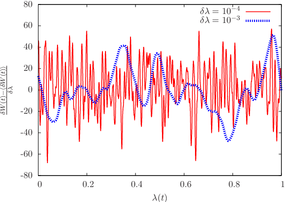
For a quasi-static process, the total work does not fluctuate because the integral (27) is computed over an infinite time such that the fluctuations in are completely integrated out.
3.3 Verifying Crooks’ relation
Since we perform a finite amount of realizations of the experiment, we can probe Crooks’ fluctuation theorem empirically only for values of where and significantly overlap.

On figure 8, we plotted the ratio for for various values of the switching rate. The line represents what we would expect from Crooks’ relation, namely . The temperature is given by (11) and is 0.3 for and the reversible work is the value of for which and can be obtained from figure 3. When both and are sufficiently large, their ratio satisfies Crooks’ relation (4).
As can be seen on figure 9, the distribution of the work is Gaussian. As pointed out in [3], in that case we can simplify Crooks’ relation. If we write the distribution of the work performed during the forward and the backward process as a Gaussian
| (32) |
then, the ratio appearing in Crooks’ relation becomes
| (33) |
and Crooks relation (4) can be valid only if the variances for the forward process and the backward process are equal: , so that the term in vanishes in the exponent and that the factor in front of the exponential is 1. By identification, we can express the inverse temperature and the reversible work in terms of the means and the variance of the work distributions:
| (34) |
and
| (35) |
These relations enable us to probe the validity of Crooks’ relation in the Gaussian case even if the distributions for the forward process and the backward process don’t overlap.
The dissipated work ( for the forward process and for the backward process) is then also Gaussian, and its mean is related to its variance by
| (36) |
This relation can be seen as a generalization of the equilibrium fluctuation dissipation theorem. The mean dissipation is proportional to the fluctuation of the dissipation and the proportionality coefficient is the temperature, just as in the equilibrium fluctuation dissipation theorem.
As a consequence of eq. (36), the quantity
| (37) |
is Gaussian with zero mean and unit variance, independently of the values of and .

On figure 9, we can see the distribution of for various values of and , for the forward and for the backward process. As we can see on this figure, the distributions of coming from simulations performed with different values of the switching rate and of the fluctuation parameter all collapse onto a Gaussian distribution with zero mean and unit variance From that, we can conclude that and are Gaussian, that the system satisfies Crooks’ relation (4) or equivalently (36), and that the temperature and the reversible work are correctly given by Crooks’ relation or equivalently by equations (34) and (35).
4 Summary and outlook
We have presented a basic numerical experiment which permits to probe the validity of Crooks’ fluctuation relation on the fluctuating lattice-Boltzmann model. We have seen that this model fulfills Crooks’ relation and that in this particular situation, Crooks’ relation is considerably simplified due to the Gaussian nature of the distribution of the work performed during the switching. This simplification enables us to probe Crooks’ relation, even in situations where and do not overlap significantly.
This experiment suggests that the FLBM is thermodynamically consistent. The reversible work depends only on the initial and final states, that is on and . The mean dissipated work depends only on the switching rate . The fluctuations depend on the fluctuation parameter and on the switching rate . Even though this model has no a priori well defined energy or free energy, one could define the free energy (up to an additive constant) using (35). However, the link between this quantity and the microdynamics of the system is still to determine.
The fluctuating lattice-Boltzmann model is a very simple model for a thermal gas. It enables us to study Crooks’ fluctuation relation in a simple situation. Equation (27) suggests that the interesting quantity is . Its value during the process only depends on the instantaneous mass density distribution . One could, for instance, study the fluctuations in around its mean value during the switching and compare them to the equilibrium fluctuations. More generally, this model could help identify the sources of dissipation in a finite switching-time experiment or in a non-equilibrium steady state and the link between fluctuation and dissipation in non-equilibrium situations.
References
References
- [1] Crooks G A. Nonequilibrium measurements of free energy differences for microscopically revresible Markovian systems. J. Stat. Phys., 90:1481, 1998.
- [2] Jarzynski C. Nonequilibrium Equality for Free Energy Differences. Phys. Rev. Lett., 78:2690, 1997.
- [3] Douache F, Ciliberto S, and Petrosyan A. Estimate of the free energy difference in mechanical systems from work fluctuation theorems. J. Stat. Mech., page P09011, 2005.
- [4] Andrieux D, Gaspard P, Ciliberto S, Garnier N, Joubaud S, and Petrosyan A. Thermodynamic time asymetry in non-equilibrium fluctuations. J. Stat. Mech., page P01002, 2008.
- [5] Harris R J and Schuetz G M. Fluctuation theorems for stochastic dynamics. J. Stat. Mech., page P07020, 2007.
- [6] Succi S. The lattice Boltzmann Equation : for Fluid Dynamics and Beyond. Oxford New York: Oxford University Press, 2001.
- [7] Dunweg B, Schiller U, and Ladd A J C. Statistical mechanics of the fluctuating lattice Boltzmann equation. Phys. Rev.E, 76:036704, 2007.
- [8] Dunweg B and Ladd A J C. Lattice Boltzmann simulation of soft matter systems. Adv. Polymer Sci., 80:221, 2009.
- [9] Dunweg B, Schiller U D, and Ladd A J C. Progess in the Understanding of the Fluctuating Lattice Boltzmann Equation. Computer physics comunications, 180:605–608, 2009.